
Optimisation of the Magnetic Circuit of a Measuring Head for Diagnostics of Steel-Polyurethane Load-Carrying Belts Using Numerical Methods


Abstract
:1. Introduction
- loss of metallic cross-section,
- permissible amount of steel wire scrap,
- change in load-carrying belt dimensions,
- degree of deformation,
- wear of integral load-carrying belt material.
2. Testing Methodology
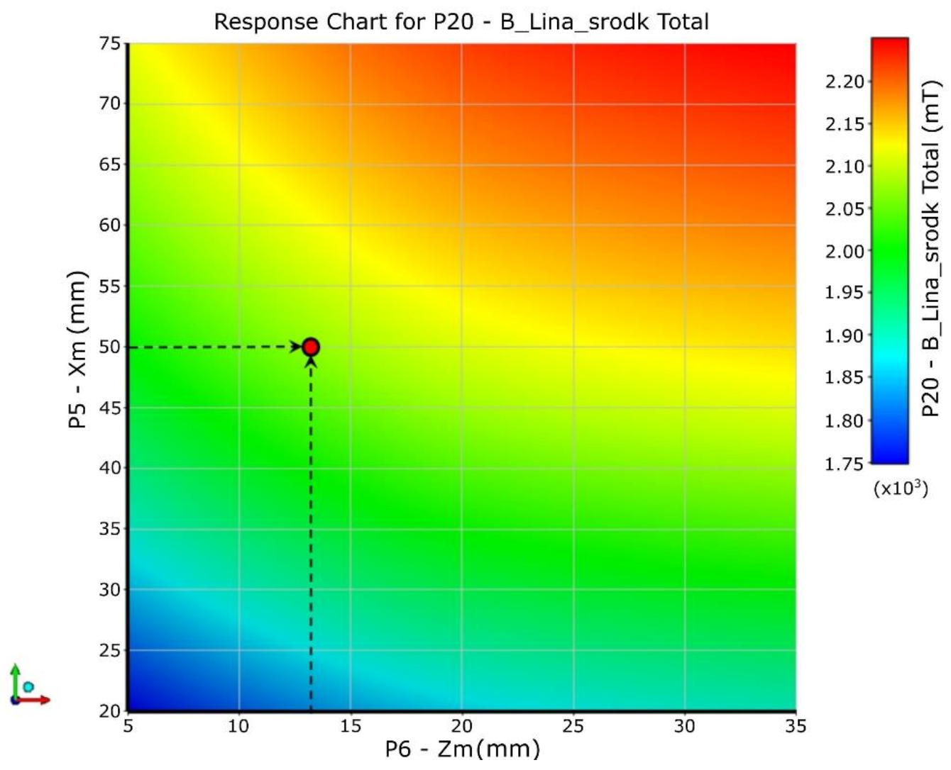
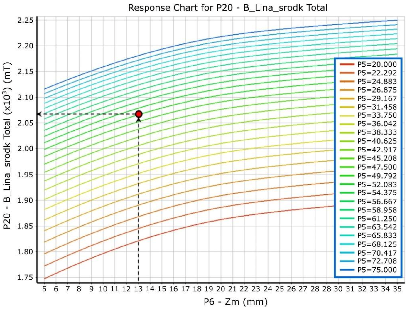
3. Magnetic Circuit Optimisation Using Numerical Analyses
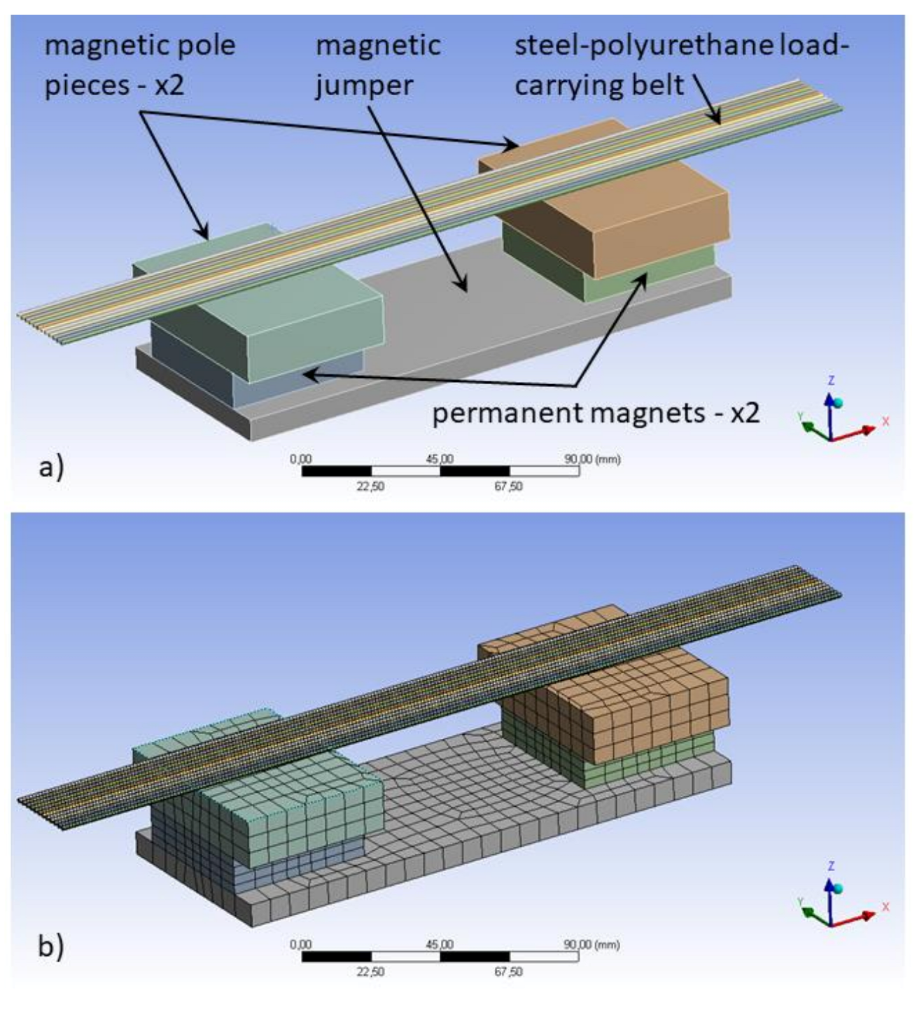
- 2 oppositely polarised permanent magnets of NdFeB (neodymium-iron- boron) type,
- 2 pole pieces distributing the magnetic flux to a load-carrying belt,
- a magnetic jumper to close the magnetic circuit from below, and
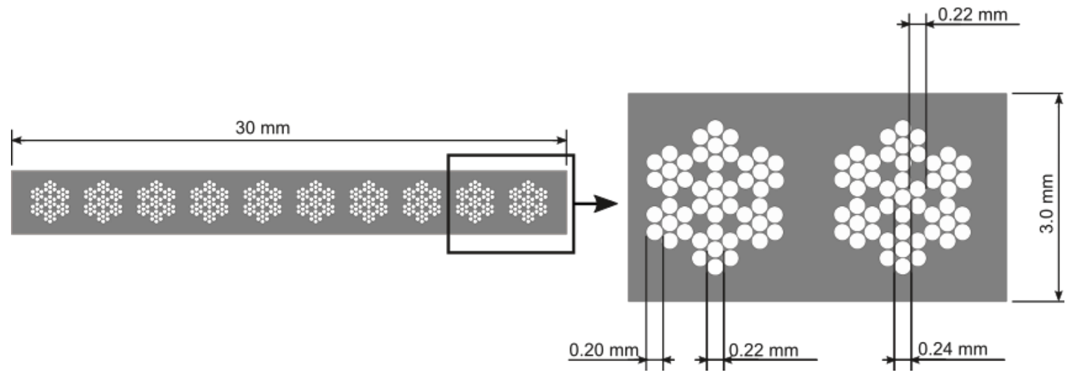
- 12 steel wire ropes forming a load-carrying cable (belt).
- In real measurements, an inaccuracy of at least 0.5 mm in the measuring probe location in the ambient space in relation to a point from the numerical analysis may lead to significant discrepancies in the identified value of total induction.
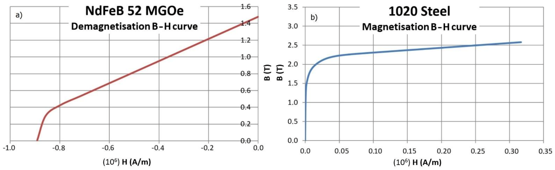
- For numerical analyses, the publicly available magnetic data (primary magnetisation curve BH) for the general-purpose ferritic structural steel was used—the actual magnetisation curve of the structural material was not verified in the laboratory. The same procedure was followed for the hard magnetic material (permanent magnet), trusting the magnet parameters declared by the manufacturer. Only the value of the perpendicular component of magnetic field induction to the magnet pole 3 mm above its surface was verified, obtaining a value of approximately 273 mT from the actual measurement and approximately 270 mT from the numerical simulation of a free magnet in the air space.
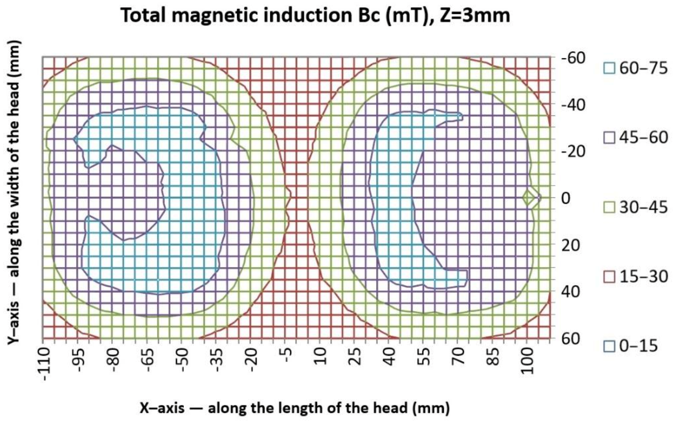
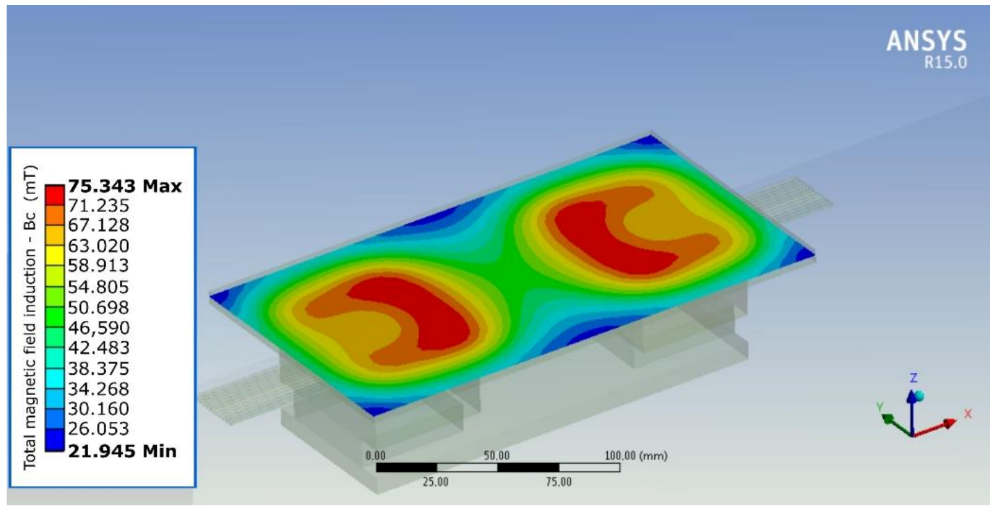
- The numerical analysis is an idealised analysis as opposed to a real magnetic circuit. The magnetic circuit elements in the FEM analysis were represented as cuboidal elements with perfectly smooth walls and edges. The actual magnetic circuit was tailored for a useful measuring device and therefore had additional technological holes allowing for the installation of sockets, sensor elements, housings, etc. These small changes and violations of geometry continuity also had little effect on the magnetic field distribution as can be seen in Figure 10, in relation to the ideal and symmetrical magnetic field distribution from the FEM analysis in Figure 11.
- The actual measurement was carried out at points with the resolution of 5 mm in the X and Y axes in the measurement plane, unlike the numerical analysis in which the data were taken continuously from the XY plane.
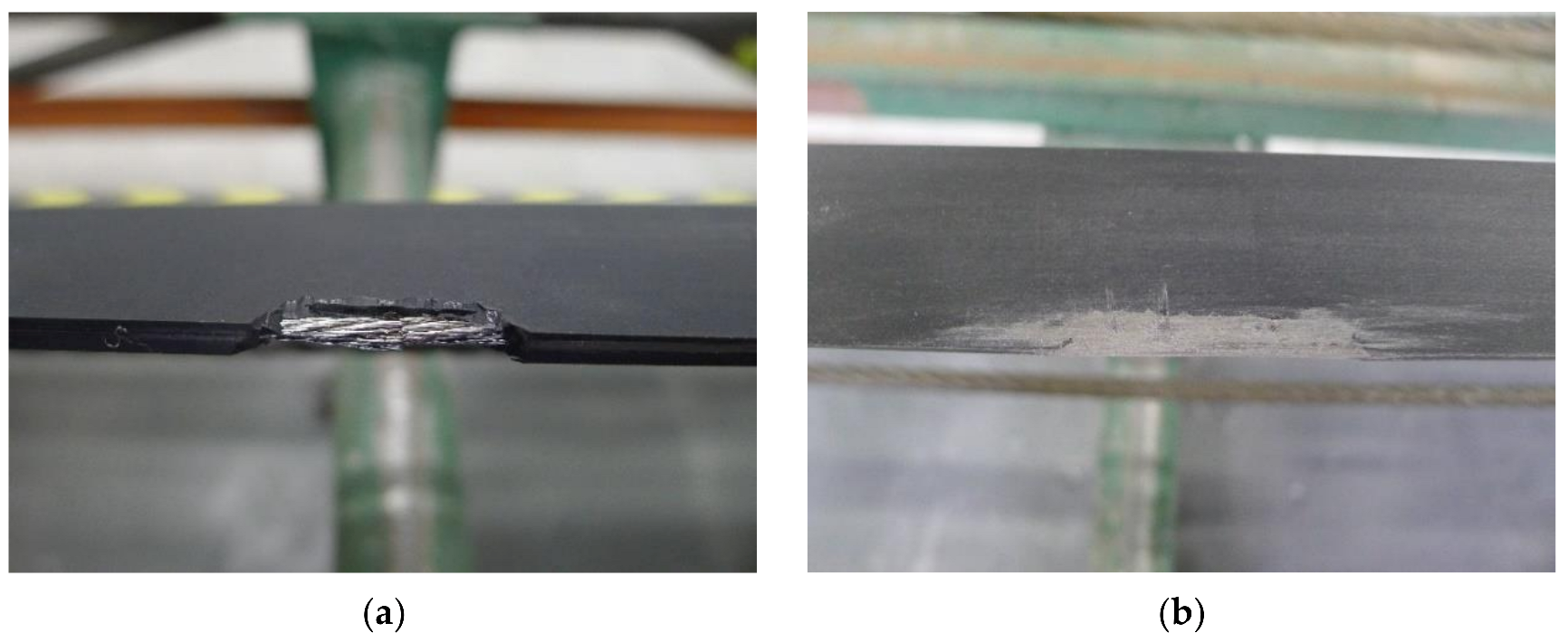
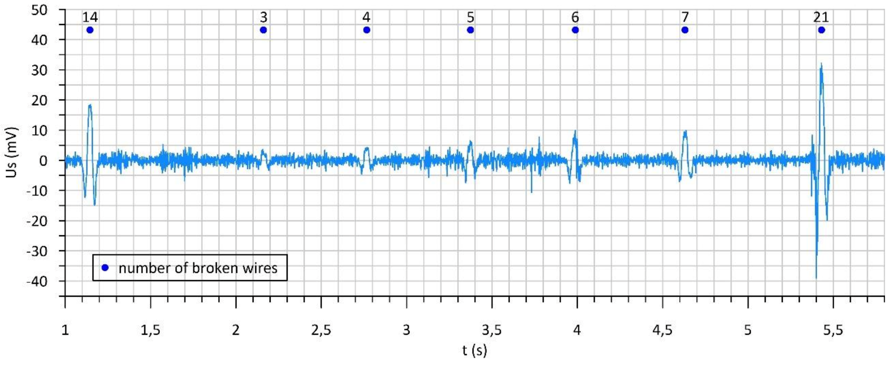
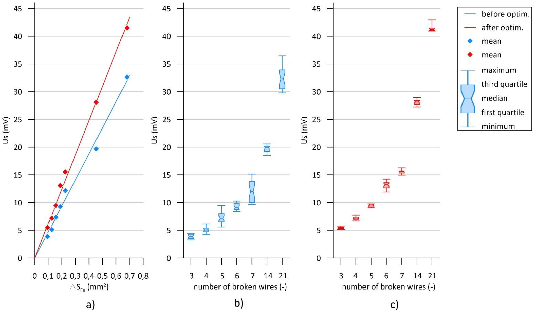
4. Verification Tests
5. Discussion
6. Conclusions
- The use of simulation methods in various fields of mechanical engineering allows for a significant reduction of the optimisation process time and minimisation of costs associated with intermediate prototypes. Numerical simulations are used not only to optimise the structures in terms of mass or safety-related indices, but also to model, analyse, and optimise the magnetic circuits.
- The optimisation of magnetic circuit made it possible to optimise the magnetic head in terms of metrological properties as well as mass and size criteria. Appropriate selection of the parameters of magnets, air gap, and other circuit elements made it possible to obtain the magnetic field induction in wire ropes of the tested load-carrying belt having the values close to magnetic saturation of their material.
- The correctness of numerical analyses carried out was confirmed by comparing the results obtained with actual measurements of the magnetic field induction in the vicinity of the magnetic circuit.
- The improved functional properties and the reduced weight were also achieved by using 3D printing technology.
- The optimisation of magnetic circuit and the modernisation of existing measurement head prototype resulted in a better quality of the recorded signal. The signals recorded with the optimised head have a higher signal-to-noise ratio. Thanks to this, it is possible to more easily locate defects with a small loss of metallic cross-section, which until now, due to the value of the signal associated with the defects, was drowned out by the noise component of the signal recorded.
- The comparative measurements carried out in the laboratory were performed under the same measuring conditions and with the same operating parameters. The obtained results allow a more metrologically and ergonomically effective application of the optimised head on real lifting devices.
- In order to confirm the obtained results, further work on the magnetic circuit should be extended to other optimization procedures.
- The obtained results under laboratory conditions should be further confirmed on real devices with different support tendons.
Author Contributions
Funding
Institutional Review Board Statement
Informed Consent Statement
Data Availability Statement
Conflicts of Interest
References
- PN-EN. 81-20:2020 Safety Rules for the Construction and Installation of Lifts-Lifts for the Transport of Persons and Goods-Part 20: Passenger and Goods Passenger Lifts; Poland, 2020. [Google Scholar]
- GEN2. Technology for Your Existing Building. Available online: https://www.otis.com/documents/256045/6552829/OTIS-Gen2MOD_Final.pdf/b2d0ba43-491b-7ae7-ec73-a710f9d7ba9e?t=1594735223630 (accessed on 9 December 2021).
- Conti Polyflat. Available online: https://www.continental-industry.com/getmedia/267f7e79-d50f-48a2-9b3b-934b03d7f236/PTG9267-EnDe_POLYFLAT.pdf (accessed on 9 December 2021).
- Kwaśniewski, J.; Krakowski, T. Intelligent diagnostic system of flexible polyurethane–coated steel belts. Transp. Logist. 2010, 7, 210–215. [Google Scholar]
- Kwaśniewski, J.; Ruta, H. The design of magnetic circuits taking into account measuring application. Electr. Rev. 2011, 87, 60–65. [Google Scholar]
- Krakowski, T.; Molski, S.; Ruta, H.; Lonkwic, P.; Tofil, A. Diagnostics of operational wear in hybrid load-carrying cables. J. Phys. Conf. Ser. 2021, 1736, 012012. [Google Scholar] [CrossRef]
- Lonkwic, P.; Krakowski, T.; Ruta, H. Application of stray magnetic field for monitoring the wear degree in steel components of the lift guide rails system. Metals 2020, 10, 1008. [Google Scholar] [CrossRef]
- Mańka, E.; Styp-Rekowski, M. Porównanie wybranych wielkości wykorzystywanych do oceny stanu lin określonych różnymi metodami. Stud. Proc. Pol. Assoc. Knowl. Manag. 2011, 47, 157–168. [Google Scholar]
- Kwaśniewski, J. Application of the wavelet analysis to inspection of compact ropes using a high-efficiency device. Arch. Min. Sci. 2013, 58, 159–164. [Google Scholar]
- Dogonchi, A.S.; Tayebi, T.; Chamkha, A.J. Natural convection analysis in a square enclosure with a wavy circular heater under magnetic field and nanoparticles. J. Therm Anal. Calorim 2020, 139, 661–671. [Google Scholar] [CrossRef]
- Sarafraz, M.M.; Pourmehran, O.; Yang, B.; Arjomandi, M.; Ellahi, R. Pool boiling heat transfer characteristics of iron oxide nano-suspension under constant magnetic field. Int. J. Therm. Sci. 2020, 147, 106131. [Google Scholar] [CrossRef]
- Malikan, M.; Krasheninnikov, M.; Eremeyev, V.A. Torsional stability capacity of a nano-composite shell based on a nonlocal strain gradient shell model under a three-dimensional magnetic field. Int. J. Eng. Sci. 2020, 148, 103210. [Google Scholar] [CrossRef]
- Zarezadeh, E.; Hosseini, V.; Hadi, A. Torsional vibration of functionally graded nano-rod under magnetic field supported by a generalized torsional foundation based on nonlocal elasticity theory. Mech. Based Des. Struct. Mach. 2020, 48, 480–495. [Google Scholar] [CrossRef]
- Hosseinzadeh, K.; Roghani, S.; Mogharrebi, A.R. Optimization of hybrid nanoparticles with mixture fluid flow in an octagonal porous medium by effect of radiation and magnetic field. J. Therm Anal. Calorim 2021, 143, 1413–1424. [Google Scholar] [CrossRef]
- Qi, C.; Tang, J.; Fan, F.; Yan, Y. Effects of magnetic field on thermo-hydraulic behaviors of magnetic nanofluids in CPU cooling system. Appl. Therm. Eng. 2020, 179, 115717. [Google Scholar] [CrossRef]
- Fleishman, G.D.; Gary, D.E.; Chen, B.; Kuroda, N.; Yu, S.; Nita, G.M. Decay of the coronal magnetic field can release sufficient energy to power a solar flare. Science 2020, 367, 278–280. [Google Scholar] [CrossRef]
- Izadi, M.; Mikhail, A.S.; Mehryan, S.A.M. Natural convection of a hybrid nanofluid affected by an inclined periodic magnetic field within a porous medium. Chin. J. Phys. 2020, 65, 447–458. [Google Scholar] [CrossRef]
- Yongbo, L.; Xiaoqiang, D.; Fangyi, W.; Xianzhi, W.; Huangchao, Y. Rotating machinery fault diagnosis based on convolutional neural network and infrared thermal imaging. Chin. J. Aeronaut. 2020, 33, 427–438. [Google Scholar]
- Tie, S.; Zhao, W.; Xin, D. Robust Fabrication of Hybrid Lead-Free Perovskite Pellets for Stable X-ray Detectors with Low Detection Limit. Adv. Mater. 2020, 32, 2001981. [Google Scholar] [CrossRef]
- Suraci, S.V.; Fabiani, D.; Xu, A.; Roland, S.; Colin, X. Ageing Assessment of XLPE LV Cables for Nuclear Applications Through Physico-Chemical and Electrical Measurements. IEEE Access 2020, 8, 27086–27096. [Google Scholar] [CrossRef]
- Jin., Y.; Walker, E.; Heo, H. Nondestructive ultrasonic evaluation of fused deposition modeling based additively manufactured 3D-printed structures. Smart Mater. Struct. 2020, 29, 45020. [Google Scholar] [CrossRef]
- Gallardo-Saavedra, S.; Hernández-Callejo, L.; Alonso-García, M. Nondestructive characterization of solar PV cells defects by means of electroluminescence, infrared thermography, I–V curves and visual tests: Experimental study and comparison. Energy 2020, 205, 117930. [Google Scholar] [CrossRef]
- Weiland, J.; Hesser, D.F.; Xiong, W. Structural health monitoring of an adhesively bonded CFRP aircraft fuselage by ultrasonic Lamb Waves. Proc. Inst. Mech. Eng. Part G J. Aerosp. Eng. 2020, 234, 2000–2010. [Google Scholar] [CrossRef]
- Roskosz, M.; Fryczowski, K.; Schabowicz, K. Evaluation of Ferromagnetic Steel Hardness Based on an Analysis of the Barkhausen Noise Number of Events. Materials 2020, 13, 2059. [Google Scholar] [CrossRef]
- Roskosz, M.; Fryczowski, K.; Tuz, L.; Wu, J.; Schabowicz, K.; Logoń, D. Analysis of the Possibility of Plastic Deformation Characterisation in X2CrNi18-9 Steel Using Measurements of Electromagnetic Parameters. Materials 2021, 14, 2904. [Google Scholar] [CrossRef]
- Molina-Viedma, A.J.; Pieczonka, Ł.; Mendrok, K.; López-Alba, E.; Díaz, F.A. Damage identification in frame structures using high-speed digital image correlation and local modal filtration. Struct. Control. Health Monit. 2020, 27, 1–16. [Google Scholar] [CrossRef]
- Kawecki, Z.; Stachurski, J. Defektoskopia Magnetyczna Lin Stalowych, 1st ed.; Wydawnictwo Śląsk: Katowice, Poland, 1969; pp. 31–89. [Google Scholar]
- Kwaśniewski, J. Badania Magnetyczne Lin Stalowych, System Certyfikacji Personelu w Metodzie MTR, 1st ed.; Wydawnictwa AGH: Kraków, Poland, 2004; pp. 59–99. [Google Scholar]
- Tytko, A. Eksploatacja Lin Stalowych, 1st ed.; Wydawnictwo Śląsk: Katowice, Poland, 2003; pp. 301–374. [Google Scholar]
- Halliday, D.; Resnick, R.; Walker, J. Basics of Physics 3; Wydawnictwo Naukowe PWN SA: Warszawa, Poland, 2003; pp. 248–251. [Google Scholar]
- Ruta, H. Zastosowanie Metod Symulacyjnych w Określaniu Właściwości Metrologicznych Urządzeń Diagnostycznych. Ph.D. Thesis, Kraków, Poland, 2018. [Google Scholar]
- Skoczylas, J. Analiza pola magnetycznego magnesu trwałego przy zastosowaniu metody elementów skończonych. Arch. Elektrotechniki 1981, nr 1, 22–30. [Google Scholar]
- Kogen-Dalin, W.W.; Komarow, E.W.; Zadrożny, J. Obliczanie i badania układów z magnesami trwałymi; Wydawnictwa Naukowo-Techniczne: Warszawa, Poland, 1982. [Google Scholar]
- Bolkowski, S.; Stabrowski, M.; Skoczylas, J.; Sroka, J.; Sikora, J.; Wincenciak, S. Komputerowe Metody Analizy Pola Elektromagnetycznego; Wydawnictwa Naukowo–Techniczne: Warszawa, Poland, 1993. [Google Scholar]
- Meeker, D. Finite Element Method Magnetics Version 4.2 FEMM Material Database; University of Virginia: Charlottesville, VA, USA, 2015. [Google Scholar]
- Moaveni, S. Finite Element Analysis Theory and Application with ANSYS; Pearson Education, Inc: Hoboken, NJ, USA, 2008. [Google Scholar]
- Sikora, J. Numeryczne Metody Rozwiązywania Zagadnień Brzegowych-Podstawy Metody Elementów Skończonych i Metody Elementów Brzegowych; Wydawca, Politechnika Lubelska: Lublin, Poland, 2011. [Google Scholar]
- Reh, S.; Beley, J.D.; Mukherjee, S.; Khor, E.H. Probabilistic finite element analysis using ANSYS. Struct. Saf. 2006, 28, 17–43. [Google Scholar] [CrossRef]
- Serageldin, A.A.; Abdelrahman, A.K.; Ookawara, S. Parametric study and optimization of a solar chimney passive ventilationsystem coupled with an earth-to-air heat exchanger. Sustain. Energy Technol. Assess. 2018, 30, 263–278. [Google Scholar]
- Thacker, V.; Vijayaragavan, E. Design optimization of clutch cushion disc with the integration of finite element analysis and design of experiments. IOP Conf. Ser. Mater. Sci. Eng. 2018, 402, 12053. [Google Scholar] [CrossRef]
- Popella, H.; Henneberger, G. Design and optimization of the magnetic circuit of a mobile nuclear magnetic resonance device for magnetic resonance imaging. COMPEL Int. J. Comput. Math. Electr. Electron. Eng. 2001, 20, 269–279. [Google Scholar] [CrossRef]
- Malarska, A. Statystyczna Analiza Danych, 1st ed.; SPSS Polska: Kraków, Poland, 2005; pp. 24–39. [Google Scholar]
- Potter, K.; Hagen, H.; Kerren, A.; Dannenmann, P. Methods for presenting statistical information: The box plot. Vis. Large Unstr. Data Sets. 2006, 4, 97–106. [Google Scholar]
- Jóźwiak, J.; Podgórski, J. Statystyka od Podstaw, 7th ed.; Polskie Wydawnictwo Ekonomiczne: Warszawa, Poland, 2012; pp. 19–101. [Google Scholar]
- Zhao, H.; Zhang, C. An online-learning-based evolutionary many-objective algorithm. Inf. Sci. 2020, 509, 1–21. [Google Scholar] [CrossRef]
- Fathollahi-Fard, A.M.; Dulebenets, M.A.; Hajiaghaei-Keshteli, M. Two hybrid meta-heuristic algorithms for a dual-channel closed-loop supply chain network design problem in the tire industry under uncertainty. Adv. Eng. Inform. 2021, 50, 101418. [Google Scholar] [CrossRef]
- Dulebenets, M.A. A Delayed Start Parallel Evolutionary Algorithm for just-in-time truck scheduling at a cross-docking facility. Int. J. Prod. Econ. 2019, 212, 236–258. [Google Scholar] [CrossRef]
- Liu, Z.; Wang, Y.; Huang, P. A many-objective evolutionary algorithm with angle-based selection and shift-based density estimation. Inf. Sci. 2020, 509, 400–419. [Google Scholar] [CrossRef] [Green Version]
- Pasha, J.; Dulebenets, M.A.; Kavoosi, M. An Optimization Model and Solution Algorithms for the Vehicle Routing Problem with a “Factory-in-a-Box”. IEEE Access 2020, 8, 134743–134763. [Google Scholar] [CrossRef]
- Dulebenets, M.A.; Pasha, J.; Abioye, O.F. Exact and heuristic solution algorithms for efficient emergency evacuation in areas with vulnerable populations. Int. J. Disaster Risk Reduct. 2019, 39, 101114. [Google Scholar] [CrossRef]
- D’Angelo, G.; Pilla, R.; Tascini, C. A proposal for distinguishing between bacterial and viral meningitis using genetic programming and decision trees. Soft Comput. 2019, 23, 11775–11791. [Google Scholar] [CrossRef]


| Parameter Name | Unit | Parameter symbol | ANSYS Symbol | Initial Value | Range of Variability | Target Value | |
|---|---|---|---|---|---|---|---|
| Minimum | Maximum | ||||||
| Length of the magnetic jumper | (mm) | Xz | P1 | 195 | 150 | 250 | ? |
| Width of the magnetic jumper | (mm) | Yz | P2 | 70 | 30 | 100 | ? |
| High of the magnetic jumper | (mm) | Zz | P3 | 10 | 3 | 15 | ? |
| Length and width of the magnet | (mm) | Xm | P5 | 50 | 20 | 75 | ? |
| High of the magnet | (mm) | Zm | P6 | 13 | 5 | 35 | ? |
| Pole piece length | (mm) | Xn | P7 | 52 | 30 | 70 | ? |
| Pole piece width | (mm) | Yn | P8 | 70 | 30 | 100 | ? |
| Pole piece height | (mm) | Zn | P9 | 17 | 5 | 25 | ? |
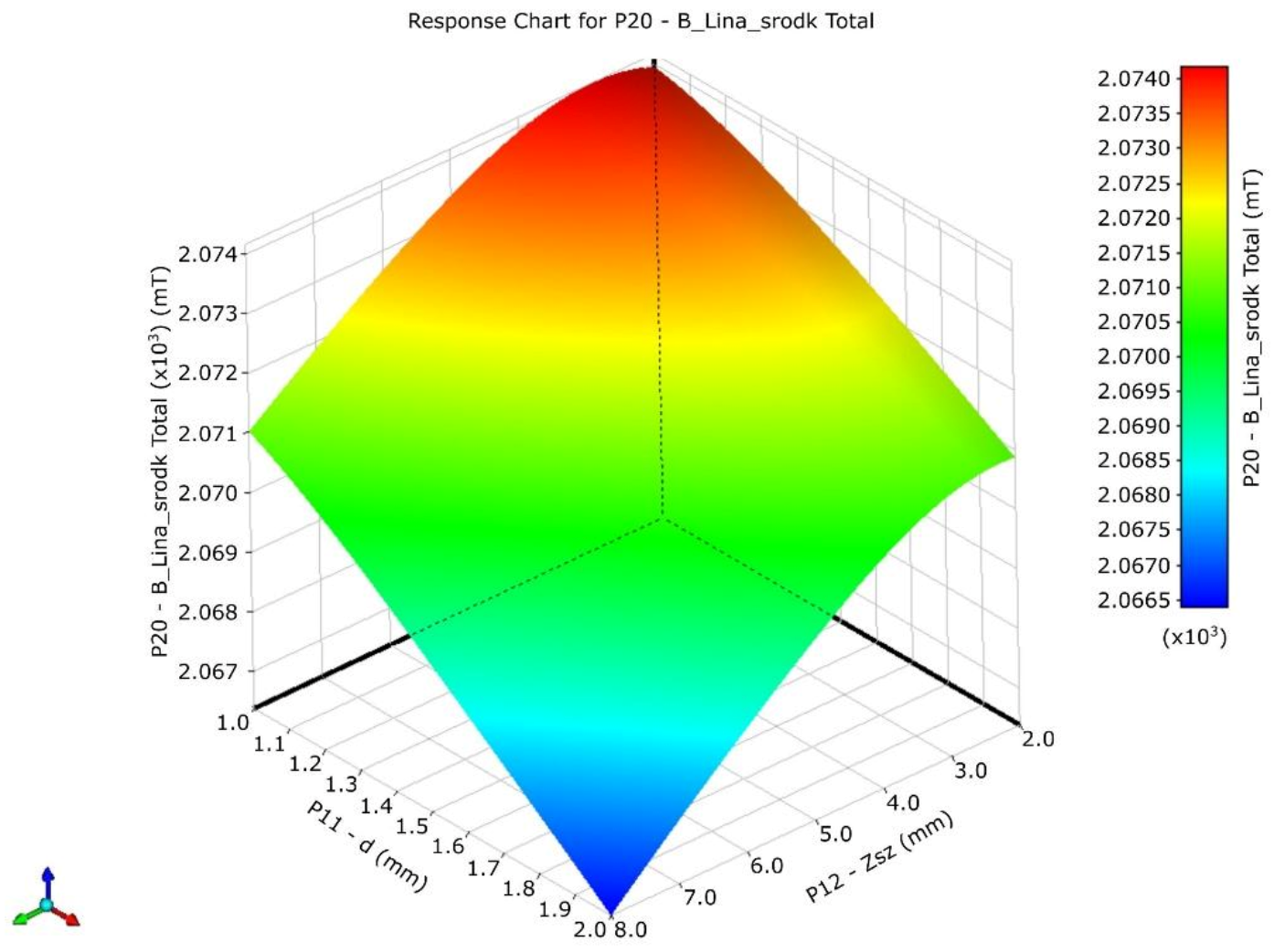
| Steel rope diameter | (mm) | d | P11 | 1.6 | 1 | 2 | ? |
| Air gap | (mm) | Zsz | P12 | 4.7 | 2 | 8 | ? |
| Parameter Name | Unit | Parameter symbol | ANSYS Symbol |
|---|---|---|---|
| Mass of the magnetic jumper | (kg) | Mz | P15 |
| Mass of the magnet | (kg) | Mm | P16 |
| Mass of the pole piece | (kg) | Mn | P17 |
| Magnetic induction—right wire rope | (mT) | Blp | P18 |
| Magnetic induction—left wire rope | (mT) | Bll | P19 |
| Magnetic induction—centre wire rope | (mT) | Bls | P20 |
| Magnetic induction in the centre of the magnetic jumper | (mT) | Bzw | P24 |
| Magnetic induction at the centre of the magnet | (mT) | Bmag | P28 |
| Magnetic induction in the centre of the pole piece | (mT) | Bnab | P32 |
| Parameter Name | Unit | Before Modernisation | After Modernisation | |||||
|---|---|---|---|---|---|---|---|---|
| X | Y | Z | X | Y | Z | |||
| Dimensions of the elements of the magnetic circuit | Magnetic jumper | (mm) | 195 | 70 | 10 | 185 | 70 | 8 |
| Pole piece | (mm) | 52 | 70 | 17 | 55 | 70 | 14 | |
| Permanent magnet | (mm) | 50 | 50 | 13 | 50 | 50 | 13 | |
| Complete magnetic circuit | (mm) | 195 | 70 | 40 | 185 | 70 | 35 | |
| Weight | Complete magnetic circuit | (kg) | 2.56 | 2.17 | ||||
| Number of Broken Wires n | Loss of Metallic Cross Section ΔSFe | |
|---|---|---|
| (-) | (mm2) | (%) |
| 3 | 0.094 | 0.58 |
| 4 | 0.126 | 0.77 |
| 5 | 0.157 | 0.96 |
| 6 | 0.188 | 1.15 |
| 7 | 0.227 | 1.39 |
| 14 | 0.453 | 2.78 |
| 21 | 0.680 | 4.17 |
| Number of Broken Wires n | (-) | 3 | 4 | 5 | 6 | 7 | 14 | 21 | |||||||
|---|---|---|---|---|---|---|---|---|---|---|---|---|---|---|---|
| Loss of metallic cross section ΔSFe | (mm2) | 0.094 | 0.126 | 0.157 | 0.1880 | 0.227 | 0.453 | 0.680 | |||||||
| (%) | 0.58 | 0.77 | 0.96 | 1.15 | 1.39 | 2.78 | 4.17 | ||||||||
| Mean signal amplitude AUs | (mV) | 3.91 | 5.48 | 5.14 | 7.22 | 7.40 | 9.47 | 9.27 | 13.11 | 12.16 | 15.54 | 19.67 | 28.09 | 32.62 | 41.47 |
| Standard deviation s(AUs) | (mV) | 0.35 | 0.17 | 0.56 | 0.31 | 1.21 | 0.27 | 0.62 | 0.65 | 2.02 | 0.34 | 0.63 | 0.48 | 2.28 | 0.67 |
| (%) | 9.00 | 3.10 | 10.96 | 4.29 | 16.30 | 2.82 | 6.69 | 4.93 | 16.59 | 2.19 | 3.18 | 1.71 | 2.28 | 1.62 | |
| Minimum signal amplitude AUsmin | (mV) | 3.30 | 5.17 | 4.26 | 6.72 | 5.61 | 9.05 | 8.42 | 11.95 | 9.66 | 14.9 | 18.48 | 27.26 | 29.77 | 40.91 |
| Maximum signal amplitude AUsmax | (mV) | 4.40 | 5.75 | 6.15 | 7.77 | 9.46 | 9.77 | 10.27 | 14.22 | 15.16 | 16.29 | 20.57 | 28.91 | 36.46 | 42.93 |
| First quartile Q1 | (mV) | 3.56 | 5.35 | 4.73 | 7.01 | 6.56 | 9.20 | 8.76 | 12.68 | 10.02 | 15.3 | 19.16 | 27.73 | 30.51 | 41.01 |
| Third quartile Q3 | (mV) | 4.30 | 5.59 | 5.38 | 7.29 | 8.04 | 9.72 | 9.86 | 13.57 | 13.79 | 15.71 | 20.18 | 28.40 | 33.9 | 41.16 |
| Quarterly deviation Q | (mV) | 0.37 | 0.12 | 0.32 | 0.14 | 0.74 | 0.26 | 0.55 | 0.44 | 1.88 | 0.20 | 0.51 | 0.33 | 1.69 | 0.07 |
| (%) | 9.48 | 2.19 | 6.41 | 1.93 | 10.27 | 2.71 | 6.07 | 3.35 | 15.64 | 1.31 | 2.56 | 1.19 | 5.24 | 0.18 | |
Publisher’s Note: MDPI stays neutral with regard to jurisdictional claims in published maps and institutional affiliations. |
© 2022 by the authors. Licensee MDPI, Basel, Switzerland. This article is an open access article distributed under the terms and conditions of the Creative Commons Attribution (CC BY) license (https://creativecommons.org/licenses/by/4.0/).
Share and Cite
Ruta, H.; Krakowski, T.; Lonkwic, P. Optimisation of the Magnetic Circuit of a Measuring Head for Diagnostics of Steel-Polyurethane Load-Carrying Belts Using Numerical Methods. Sustainability 2022, 14, 2711. https://doi.org/10.3390/su14052711
Ruta H, Krakowski T, Lonkwic P. Optimisation of the Magnetic Circuit of a Measuring Head for Diagnostics of Steel-Polyurethane Load-Carrying Belts Using Numerical Methods. Sustainability. 2022; 14(5):2711. https://doi.org/10.3390/su14052711
Chicago/Turabian StyleRuta, Hubert, Tomasz Krakowski, and Paweł Lonkwic. 2022. "Optimisation of the Magnetic Circuit of a Measuring Head for Diagnostics of Steel-Polyurethane Load-Carrying Belts Using Numerical Methods" Sustainability 14, no. 5: 2711. https://doi.org/10.3390/su14052711
APA StyleRuta, H., Krakowski, T., & Lonkwic, P. (2022). Optimisation of the Magnetic Circuit of a Measuring Head for Diagnostics of Steel-Polyurethane Load-Carrying Belts Using Numerical Methods. Sustainability, 14(5), 2711. https://doi.org/10.3390/su14052711