Activity Chains Modelling of Travellers by Using Logit Models Based on the Utility Function

Abstract

Transportation planning plays an essential role in improving the transportation system. Therefore, planners should have the ability to forecast the response of transportation demand to changes in the characteristics of the travellers. This has led researchers to work on more effective behavioural models by updating conventional models and replacing them with activity-based modelling to describe the daily activity chains performed by travellers. So, this study uses the activity model to model and analyse daily activity to identify the factors affecting the activity chain. This study aims to use logit models based on the utility function for modelling the activity chains of travellers in Budapest city. At the same time, we identify the effects of various characteristics related to the traveller, trip and location in the activity chains. This paper presents the relationships between the two aspects of travel behaviour and activity chains by providing two different causal structures. The results showed that the location attribute, activity duration and activity purpose were most influential on the activity chains. This study provides good insights into activity chains behaviour of travellers. It also extends the need to incorporate activity model behaviour within these complicated processes and household and individual decision making of daily activity.

1. Introduction

An efficient transportation system and infrastructure are necessary for the growth and development of a country’s economy. Transportation planning plays an essential role in improving the transportation system. Therefore, planners and engineers should have the ability to forecast the response of transportation demand to changes in the properties of the transportation system and differences in the characteristics of the people using the transportation system. Travel behaviour models are used for this purpose; precisely, travel behaviour models predict travel characteristics and transportation services under alternative socio-economic situations and alternative transport service and land-use configurations. Therefore, there is a need for realistic representations of travel behaviour modelling. This has led researchers to work on more effective behavioural models by updating conventional trip-based models and replacing them with a more behaviourally oriented activity-based modelling approach [1,2]. Activity chain models have rapidly gained interest in the transportation research community. These models predict behaviour in several ways, including information activities and transport modes.

Researchers in [3,4,5,6,7,8,9,10,11,12,13,14] and others have used an activity-based approach to analyse the impact on travel of changes, mainly focusing on the socio-economic environment. These studies have concluded that the effect of travel behaviour processes on activity models in time and space is very complex.

In general, activity-based models focus on activities as the unit of analysis instead of trips in trip-based models. Besides that, focusing on activity chains permits the incorporation of constraints such as time constraints related to opening hours, work schedules, expected activity duration, and scheduling of activities [15,16]. Thus, activity-based models describe detailed activity schedules considering personal, household and spatial–temporal constraints [17,18].

Several studies assume that travellers, faced with a set of alternatives, choose maximum utility of choice. The choices are calculated as a function that maximizes the overall utility of a daily activity pattern within derived choice sets [19,20].

The reasons behind the choices have to be explored to understand personal decisions. Thus, choice set formation is conditional upon the context and dynamics. From this, we conclude the significance of alternatives in determining activity–travel patterns. From another point of view, household resources (e.g., income, living space, car, etc.) affect decision processes and play different roles in activity schedules [21,22].

One of the essential system designs of activity-based models [23] is discrete choice models based on random utility maximization (RUM). Activity-based travel models are viewed as the results of users maximizing their utility. These methods have emerged more recently because of the need to model travel as part of a more significant activity–travel model, and they involve relatively non-traditional (in the travel analysis field) methodologies such as duration analysis and the influence of variables on the activity chains.

This study aims to use the logit models to model the activity-based model of the travellers in the National Capital Region of Budapest. Using logit models is the most comprehensive structure for modelling discrete choices in travel behaviour analysis with the activity-based models. The mathematical framework of logit models is based on utility maximization theory [24].

This study used the multinomial logit model, nested logit model, and a generalized nested logit model based on the utility function to identify, analyse and model the activity chains. At the same time, we analysed and identified the effects of the different characteristics related to the traveller, trip and location on the activity chains. The relationships between the two aspects of travel behaviour and activity chains are represented in this study by providing two different causal typologies and structures and analysing the activity chains by using the logit models.

The study is organized as follows: The next section offers a theoretical background. The third section presents the methodology. The fourth section covers the study area, interview technique, model specification, and descriptive analysis. Section 5 presents model estimation results and utility function analysis, and Section 6 concludes the paper by highlighting some of the research results.

2. Theoretical Background

Over recent years, the activity-based model has received increasing attention among transportation researchers. Specifically, researchers have relied on activity-based models to overcome some of the weaknesses of the travel demand models. The activity-based model has provided a better theoretical underpinning of travel behaviour research. It addresses the questions of why people travel and how decisions regarding trips are made [25,26]. The activity-based models do not describe single-dimensional decisions concerning one trip but rather address complex decisions concerning multiple dimensions of various trips and activities. Specifically, they describe what activities are performed during a specific period, and in what destinations, at what times and in which sequence. Such activity sequences imply trips with a particular origin and destination made at a specific time of day and using a specific mode. The development of activity-based models has become increasingly significant in light of increasingly complex travel behaviour, leading to changes in activity and travel behaviour models. Therefore, transportation researchers have extended this model by explicitly emphasizing the relationship between activities and travel behaviour. This has led to research of several fields in the context of trip chain and activity participation, which can be considered the points of activity-based research in transportation [26].

The first field is that travel is a derived demand from travellers’ needs. Thus, the characteristics of travel strongly influence individual travel behaviour and the activity chains. The activities performed depend on an individual’s physiological, economic and social needs, etc. In this field, some studies capture individual activity/travel models by focusing on the mechanism by which personal activities are generated, and the factors that affect the activities, e.g., Dharmowijoyo et al. [27] focused on the activity–travel behaviour of individuals from the Jakarta. Their analysis indicated that compared to workers and students, non-workers were making fewer trips, had a lower dependency on personalised modes, were involved in a smaller number of trip chains, and were allocating less time for travelling. M. Manoj and Ashish Verma [28] presented exploratory and statistical analyses of the activity–travel behaviour of non-workers in Bangalore city. This study summarised the socio-demographic characteristics and the activity–travel behaviour of non-workers using primary activity–travel survey data collected by the authors. Arentze and Timmermans [22] developed a model of dynamic activity generation based on the assumption that individuals’ activities are driven by a limited set of needs that tend to grow over time and are influenced by activities. The utility of activity increases with the requirements it satisfies and decreases with the needs it induces. Needs are defined on the household and individual levels, and a single activity could have an influence on multiple needs simultaneously.

A second important field of the activity-based approach is that activity performance depends on the availability of specific facilities, which sets limitations to the possibilities of performing activities. In addition to that, the duration of activities and constraints concerning their sequence, the available facilities, the hours at which they are accessible, and the travel times between facilities affect which activities can eventually be performed. Many studies have dealt with the availability of specific facilities, such as limitations termed space–time constraints, to explain how these facilities affect activity performance. For instance, Liangpeng et al. [29] investigated both multiactivity and multiperson interactions in urban nuclear families. They proposed the novel concepts of “activity-restriction degree” and “activity-constraint niche” to quantify the degree of space–time constraints within time geography. The models created in this study demonstrate which activity–travel transfer was optimized at the space–time level, and that families engaged in behavioural-agent transmission effectively completed the necessary tasks even under constraints. Steven Farber et al. [30] proposed a method for measuring the social interaction potential of a metropolitan area based on the time–geographic concept of joint accessibility. The metric is sensitive to prevailing land-use patterns and commuter flows in the metropolitan area, time budgets, and the spatial distribution of common activity locations. It is calculated via a geocomputation routine in which a representative subset of after-work, space–time prisms are intersected with each other. Kang and Chen [31] developed a method of constructing a feasible region in the space–time dimension of the Household Activity Pattern Problem (HAPP). Based on the definition of an activity and its spatial and temporal constraints, a feasible space–time region for completing one activity is derived. Then, a full-day, feasible, space–time region is determined as an intersection of a set of feasible areas for activities to be performed.

A third field of the activity-based model emphasizes the household as the decision-making unit. As most households consist of multiple persons, interpersonal linkages influence activity patterns. In this context, there have been theoretical and empirical works which explain the interaction of relationships between household members. Srinivasan and Bhat [32] also considered joint participation accommodating intra-household and inter-household interactions in activity–travel behaviour analysis and examined the generation, location, and scheduling of joint activity episodes. This analysis highlights the high levels of joint activity–travel participation by individuals. Chinh Ho and Corinne Mulley [33] examined individuals’ trip chaining, with joint household travel being explicitly incorporated within a nested logit model and a typology of tours that captures various patterns of household interactions. Situational factors, represented by travel purpose, travel party composition, type of working hours, and schedule synchronisation, are critical to understanding intra-household interactions in travel trip chaining.

A fourth field of the activity-based model is that travel should be regarded in the context of activity chains, consisting of multiple activities and trips. Some studies considering the activity chains, which consist of multiple activities and trips of individual and household travel behaviour, have been conducted. For example, François and Catherine [15] proposed a typology of trip chains based on the spatial–temporal structure of trips and activity type at the destination. Anchor points, loops and dominant activities are defined and used for classification purposes. A hierarchical classification of simple and complex trip chains is derived and used to measure the occurrence of typical trip chaining behaviours among an active population segment, people aged 25–44 years old. Jianchuan Xianyua [14] presented a mathematical model to investigate the decision order of travel mode choice and trip chaining in work tours. Then, they examined how much variation in this interrelationship can be captured by explanatory variables at the individual and household levels by applying the co-evolutionary approach. Results from this study provided methodological and empirical evidence that could lead to approaches for simultaneously predicting commute mode and trip chaining behaviour. João de Abreu [16] studied the relationships between the number of complex chains (with one or more intermediate stops) and simple chains, and total distances travelled by mode and land-use approach both at the residence and the workplace using path analysis. The results confirmed the association between complex chains and higher levels of car use. Land-use patterns significantly affect travelled distances by mode directly via the influence of longer-term decisions such as vehicle ownership.

As for the last field, it is mentioned that travel and activities can be considered the outcome of a scheduling process. Activity demands are matched against a supply side, defined by the available facilities, time windows and transportation options. Besides activity-based modelling, various researchers have investigated specific temporal aspects of activity scheduling processes. Some recent studies in this field include Khandker Habib [19], who presented a comprehensive utility-based system of activity–travel scheduling options modelling (CUSTOM) and applied it to simulate workers’ daily activity–travel demand. CUSTOM used a random utility-maximising econometric approach for jointly modelling activity type choices, time expenditure choices and location choices. Ben-Akiva and Abou-Zeid [17] highlight the necessity of considering the 24-h cycle in modelling workers’ skeleton activity–travel schedule formation but applying only a discrete choice model to model departure time choices for activities. Cirillo and Axhausen [18] proposed a dynamic activity choice and scheduling model that incorporated state-dependency of choice in a framework that has similarities with extended tour-based models in the Bowman and Ben-Akiva [34] tradition. They described an estimation of the model on the Mobidrive multi-week dataset.

Most of the above studies on the activity model lack the connection among essential areas of the activity-based model that affect trip chains, activity behaviour and travel decisions. Simultaneously, trip chain and activity behaviour are estimated and analysed based on one or some factors, which do not match the actual travel choice behaviour.

Based on the previous studies, we introduce in this paper a comprehensive study to estimate, analyse and model the activity chains of travellers in Budapest.

In this study, we have used a wide range of variables to analyse and model activity chains within daily activity by using three models, a multinomial logit model, nested logit model and generalized nested logit model. Simultaneously, we calculate the utility maximum of the choice of the activity chain of travellers based on the utility function. The utility function provides an indication based on the trip, location, and factors related to travellers, and which activity chain has a high utility to the travellers. Besides that, this method helps to develop transportation planning in Budapest city, which is the best way to move towards sustainable transportation.

3. Methodology

We aim to support travel behaviour and daily activity chain choice of travellers and to understand the interaction between individuals and interaction within the household and interrelationships between the travellers and various parameters. Therefore, the activity chain model has become essential for modelling and analysing travel behaviour within the activity chains during daily activity.

Therefore, this research aims to explore activity chain behaviour and travel behaviour in Budapest Metropolitan Region, Hungary. The methodology proposed in this study can be divided into four steps. They are preparation of the database, analysis of activity chains and modelling of activity chain choice. The first step involves identifying activity chains based on the purpose, determining the number of activities per activity chain based on the type, identification of the primary activity, and typology of activity chains and structure. The second step is to create the utility function based on the different variables. The third step is to analyse the activity chains based on a wide range of variables (24 variables), identify which variables have a great influence on the activity chains, and identify the interactions between activity chains and the variables using the logit models based on the utility function. The fourth step is modelling the activity chain choice.

The discrete choice process can be easily explained by a random utility model. For this study, we used the multinomial logit, the nested logit, and a generalized nested logit model based on the utility function to reach the maximum utility of the activity chain choice. These logit models are used to model the activity chain choice model by using identified trip chain choices as alternatives. The methodology adopted for the activity chain model is presented below.

3.1. Activity Chain Theory and Classification

Activity chain is defined as every activity chain that starts at the home location and ends at the same point with one or more intermediate activities. If these activities include mandatory activities such as work/study, they are considered the primary activity; otherwise, the activity which takes the longest duration is called the primary activity. All other activities conducted in between the home and the primary activity are considered secondary activities. Thus, the activity chain can have a home, primary activity and one or more secondary activities. In this study, activity chains are classified as simple, complex and open chains. Simple chains are the simplest form of activity chains that contains two trips and one activity in-between. Complex chains include all trip chains with at least two activities. Open chains are those in which information on starting or closing trips is missing. The condition used to determine and construct the activity chains is that every activity chain will start and end on the same day.

We redefined the original dataset’s activity purpose variable into four broad activity groupings [35]:

• Subsistence—out-of-home work, school and college;
• Maintenance—out-of-home shopping, personal and appointments;
• Discretionary—out-of-home free-time, visiting;
• Home—unspecified activities in the home.

3.2. Activity Chain Typology

For our analysis, a refinement in the previous typology has been performed based on the activity purpose. An activity chain typology is proposed in this study based on earlier research [36,37,38,39] and the data obtained from the activity–travel survey. This typology is as follows;

• Simple subsistence chains (one subsistence activity in between home ends);
• Simple maintenance chains (one maintenance activity in between home ends);
• Simple discretionary chains (one discretionary activity in between home ends);
• Open subsistence chains (one subsistence activity from home);
• Open maintenance chains (one maintenance activity from home);
• Open discretionary chains (one discretionary activity from home);
• Complex chains are classified as complex subsistence chains (more than one subsistence activities in between home ends);
• Complex maintenance chain (more than one maintenance activity other than subsistence in between home ends);
• Complex discretionary chain (more than one discretionary activity other than subsistence in between home ends);
• Complex to subsistence (complex subsistence chain with one or more maintenance or discretionary activities before the subsistence);
• Complex from subsistence (complex subsistence chain with one or more maintenance or discretionary activities after subsistence activities);
• Complex to and from subsistence (complex subsistence chain with one or more maintenance or discretionary activities before and after the subsistence activities);
• Complex at subsistence (complex subsistence chain with one or more maintenance or discretionary activities in between subsistence activities);
• Complex at and from subsistence (complex subsistence chain with one or more maintenance or discretionary activities between and after the subsistence activities);
• Complex to, from and at subsistence (complex subsistence chain with one or more maintenance or discretionary activities before, after and in between the subsistence activities).

3.3. The Hypothesizes of Study

The literature review identifies the essential elements that influence the activity chain, which involves individual and household variables, trip variables, activity variables, and location variables [38]. In addition to that, the activity model predicts the choice of the activity chain, which has a high utility by travellers based on the utility function [24]. Therefore, the alternatives considered for the model as dependent variables were open chains, simple chains and complex chains. Additionally, in this study, the independent variables considered were the individual and household variables, trip variables, activity variables and the location variables [21]. The variables in the model with the highest accuracy were selected as the final data of Budapest city’s daily activity.

According to that, in this study, five formal hypotheses are investigated as the basis of establishing the role of the various variables of travellers as an impact on the decision of travellers regarding the activity chain when performing daily activity:

• The first hypothesis: the potential influences on the activity chain are investigated through the individual variables;
• The second hypothesis: the potential influences on the activity chain are investigated through the household variables,
• The third hypothesis: the potential influences on the activity chain are investigated through the trip variables;
• The fourth hypothesis: the potential influences on the activity chain are investigated through activity variables;
• The fifth hypothesis: the potential influences on the activity chain are investigated through the location variables.

By investigating the hypotheses, we can gain insight into how individuals choose the activity chain and the activity duration. We also create the utility function for the activity chain from the characteristics that affect the activity chain. Consequently, we perform analysis of this impact on the activity chain.

3.4. The Activity Chain Structure Description for Model Analysis

The multinomial, nested, and generalized nested logit models can be depicted by a tree structure representing all the alternatives. The multinomial logit model treats all alternatives equally, whereas the nested logit model and generalized nested logit include intermediate branches that group alternatives, as shown in Figure 1.

An activity chain’s structure is proposed in this study based on earlier studies [36,37,38,39] and the data obtained from the activity–travel survey. Therefore, the refinement in the structure is performed based on the activity purpose. Figure 1 and Figure 2 shows the structure of proposed activity chain patterns.

The differences in structure can result in dramatically different activity chain projections and diversions to those obtained by the multinomial logit model in cases. The nested and generalized nested logit is significantly different from the multinomial logit models because the nested and generalized nested logit models allow for the correlation among alternatives a nest. In contrast, alternatives in different nests remain independent. In other words, a greater degree of choice substitution is allowed within nests than between nests [38].

Figure 2 presents a nested structure involving three activity chains: the simple, complex, and public open, according to the nested structure groups, the subsistence, maintenance and discretionary as subchoices of the composite simple (or complex or open) activity chain. This structure permits a change in the utility of one of the simple activity chains (say, the subsistence) to affect the share of the other activity chain (i.e., maintenance) to a greater degree than a chain (in this case, the discretionary) that does not belong to the complex nest. In other words, a greater degree of choice substitution is allowed within nests than between nests [39,40].

Further, the analysis provides insights into the relationship between the individual and household variables, trip variables, activity variables, location variables, and activity chain model. This analysis aims to capture the effect of those variables on travellers into the activity chain behaviour and generate a basis for model development of activity chains [41].

3.5. The Utility Function Formulation

The utility maximization model provides a link by which choice probabilities can be estimated given variables of the activity chains, the travellers and the location. This model assumes that an individual acts to maximize their utility by choosing among the available alternatives. The utility can be formulated as a function of the traveller and the activity chain variables. Conventionally, the utility of an alternative, U_ij, is assumed to be the sum of a deterministic component, V_ij, which describes the variables of individual i and the attributes of alternative j, and a random term, ϵ_ij, which represents elements not measured, the utility function included in the model, as Equation (1):

U_ij = V_ij + ϵ_ij

(1)

The measured and included component of the model is represented by a linear additive Equation (2) that includes parameters, β, and variables, X_ij, which are predetermined functions of the characteristics of individual i and the attributes of alternative j:

U_ij = β′X_ij + ϵ_ij

(2)

The utility function of the activity chain U_{activity chain} is computed as the sum of all travel utilities U_trav,mode(i), plus the sum of activity factors utility U_{Activity,Fac(i)}, plus the sum of individual characteristics utility U_IC(i), plus the sum of household characteristics utility U_HC(i) and plus the sum of location utility V_L(i), which is described by Equation (3):

$${\mathrm{U}}_{activity chain}={{\displaystyle \sum }}_{i=0}^{N-1}{U}_{trav, mode\left(i\right)}+{{\displaystyle \sum }}_{i=0}^{N-1}{U}_{Activity,Fac\left(i\right)}+{{\displaystyle \sum }}_{i=0}^{N-1}{V}_{IC\left(i\right)}+{{\displaystyle \sum }}_{i=0}^{N-1}{V}_{HC \left(i\right)}+{{\displaystyle \sum }}_{i=0}^{N-1}{V}_{L \left(i\right)}$$

(3)

➢

The utility function of the travel variables is calculated as Equation (4):

$$\sum U_{trav, mode\left(i\right)}={\beta }_C+{\beta }_{trav, time,m}\ast T_{trav,m}+{\beta }_{C,m}{\ast \mathrm{C}}_m+{\beta }_{d,m}\ast T{D}_{trav,m}$$

(4)

where:

• β_C = is the coefficient parameter to be estimated from data for a model-specific constant,
• β_trav,time,m = is the coefficient parameter of time spent traveling by mode (m),
• t_trav,m = is the travel time between activity locations by mode (m),
• β_c,m = is the coefficient parameter of travel cost of mode (m),
• C_m = is a parameter related to of the actual travel cost for mode (m),
• β_d,m = is the coefficient parameter of the of trip distance,
• TD_trav,m = is the trip distance traveled between activity locations.

➢

The utility function of the activity variables is calculated as Equation (5):

$$\sum U_{Activity F}= {\beta }_{activity pur}\ast A{P}_{pur}+{\beta }_{activity dur}A{D}_{dur}$$

(5)

where:

• β_{activity purpose} = is the coefficient parameter of the activity purpose,
• AP_pur = is a parameter related to the activity purpose for traveller (i),
• β_{Activity dur} = is a coefficient estimated related to the activity duration,
• AD_dur = is a parameter related to the activity purpose for traveller (i).

➢

The utility function of the individual characteristics is calculated as Equation (6):

$$\sum U_{IC \left(i\right)}={\gamma }_{Gender}\ast X_{Gender}+{\gamma }_{Age}\ast X_{Age}+{\gamma }_{Mar. sta.}\ast X_{Mar. sta.}+{\gamma }_{Occ.}\ast Z_{Occ.}+{\gamma }_{Edu. level}\ast Z_{Edu. level}$$

(6)

where:

• γ_Gender = is the coefficient parameter of gender,
• X_Gender = is the parameter related to the gender (male and female) for traveller (i),
• γ_Age = is the coefficient parameter of age,
• X_Age = is a parameter related to the age for traveller (i),
• γ_{Maritual status} = is the coefficient parameter of marital status,
• X_{Maritual status} = is a parameter related to marital status of traveller (i),
• γ_Ocupation = is the coefficient parameter of the occupation,
• Z_Ocupation = is a parameter related to the occupation of traveller (i),
• γ_{Education level} = is the coefficient parameter of the education level,
• Z_{Education level} = is a parameter related to the education level of traveller (i).

➢

The utility function of the household characteristics is calculated as Equation (7):

∑U_{HC (i)} = γ_Sta.liv. ∗ Z_Sta.liv. + γ_Hou.size ∗ Z_Hou.size + γ_Hou.inc. ∗ Z_Hou.inc. + γ_{Car own.} ∗ Z_{Car own.} + γ_{Bic. own.} ∗ Z_{Bic. own.} + γ_{Mop. bike own.} ∗ Z_{Mop. bike own.} + γ_{Dri. lic.} ∗ Z_{Dri. lic.} + γ_{mon. tic.} ∗ Z_{mon. tic.} + γ_no.child. ∗ Z_no.children

(7)

where:

• ${\gamma }_{Standard living}$ = is the coefficient parameter of the standard of living of the family,
• $Z_{Standard living}$ = is a parameter related to the standard of living of traveller (i),
• ${\gamma }_{House size}$ = is the coefficient parameter of the household size (family size),
• $Z_{House size}$ = is a parameter related to the household size (family size) of traveller (i),
• ${\gamma }_{House income}$ = is the coefficient parameter of the household income,
• $Z_{House income}$ = is a parameter related to the household income of traveller (i),
• ${\gamma }_{Car ownership}$ = is the coefficient parameter of the number of car ownerships,
• $Z_{Car ownership}$ = is a parameter related to the number of car ownerships of traveller (i),
• ${\gamma }_{Bicycle ownership}$ = is the coefficient parameter of bicycle ownership,
• $Z_{Bicycle ownership}$ = is a parameter related to the bicycle ownership of traveller (i),
• ${\gamma }_{Moped bike ownership}$ = is the coefficient parameter of moped bike ownership,
• $Z_{Moped bike ownership}$ = is a parameter related to the moped ownership of traveller (i),
• ${\gamma }_{Driving license}$ = is the coefficient parameter of driving license,
• $Z_{Driving license}$ = is a parameter related to the driving license of traveller (i),
• ${\gamma }_{monthly ticket}$ = is the coefficient parameter of ticket availability,
• $Z_{mon. ticket}$= is a parameter related to the ticket availability of public transit for traveller (i),
• ${\gamma }_{no. children}$ = is the coefficient parameter of the number of the children in the household (under 12 years),
• $Z_{no.children}$ = is a parameter related to the number of children in the household of traveller (i).

➢

The utility function of the location choice is calculated as Equation (8):

$$\sum U_{L \left(i\right)}={\gamma }_{House, Location}\ast Y_{Origin, Loca.}+{\gamma }_{Destination, Loca.}\ast Y_{Destination, Loca.}+{\gamma }_{Dest., Attribute}\ast Y_{Dest., Attr.}$$

(8)

where:

• ${\gamma }_{Origin, Location}$ = is the coefficient parameter of the household location,
• $Y_{Origin, Location}$ = is a parameter related to the household location of traveller (i),
• ${\gamma }_{Destination, Location}$ = is the coefficient parameter of the destination location,
• $Y_{Destination, Location}$ = is a parameter related to the destination location of traveller (i),
• ${\gamma }_{Destination, Attribute}$ = is the coefficient parameter of the destination attribute,
• $Y_{Destination, Attribute}$ = is a parameter related to destination attribute of traveller (i).

From the equations above, one can see the linear utility function of the activity chain. It is used to estimate the utility values of each choice alternative which depend on the values of the variables associated with the alternatives [42].

Travellers’ choice means assigning the chosen value of the alternative with high utility and not the choice of another alternative with less value.

3.6. Logit Models

The logit model has the ability to model complex travel behaviours of any population with simple mathematical techniques and thus prove to be the most widely used tool for activity chain modelling. The mathematical framework of logit models is based on utility maximization theory [24,43].

3.6.1. The Multinomial Logit Model Formulation

For this study, the multinomial logit model (MNL) is used to investigate and identify the effect of the variables related to travellers on the activity chain and estimate the coefficients of the underlying model. The MNL model has the ability to model travel behaviours by using simple mathematical techniques, thus proving to be the most widely used tool for the activity chain modelling [44]. The mathematical framework of MNL model is based on utility function theory [24]. The activity chain models statistically relate the choice made by each traveller to the attributes of the alternatives available. The components of the utilities of the different set of alternatives in the MNL model are assumed to be independent. The general Equation (9) of the MNL model for the probability of choosing an alternative ‘i’ (i = 1, 2, …, J) from a set of J alternatives is:

$$\mathit{Pr}(i)=\frac{\mathit{exp}\left(U_{in}\right)}{{{\displaystyle \sum }}_{i=1}^J\mathit{exp}\left(U_{in}\right)} ,$$

(9)

where:

• Pr (i) = is probability of the activity chain (n) by traveller choosing alternative (i),
• $U_{in}$ = is utility component of activity chain (n) by traveller choosing alternative (i),
• $U_J$ = is the systematic component of the utility of the set alternative (j).

The MNL identifies how the independent variables are related to the dependent variable and is expressed in terms of utility. For each case, the traveller has the available alternatives: open activity chain, simple activity chain and complex activity chain.

3.6.2. The Nested Logit (NL) Model Formulation

The Nested logit (NL) model is a generalization of the multinomial logit model (MNL), and it characterizes a partial relaxation of the independence of the irrelevant alternatives (IIA) property of the MNL model. A nested logit model is appropriate when the subsets of similar alternatives are grouped in hierarchies or nests [45,46,47]. The NL model consists of three trunks of the activity chain, which include open activity chain, a simple activity chain and a complex activity chain. The NL model can be calibrated to find coefficients by using standard logit estimation. The hierarchical structure of the NL model such as the one represented by Equation (10) is estimated for each hierarchy [48,49,50];

$$P_{ij}=\frac{e^{U_{ij}}}{{{\displaystyle \sum }}_{i=1}^j{e}^{U_j}}$$

(10)

where:

• $P_{ji}$ = is the probability that traveller i chooses alternative j,
• $U_{ij}$ = is utility component of activity chain (n) by traveller choosing alternative (i),
• $U_J$ = is the systematic component of the utility of the set alternative (j).

The nested logit model can be illustrated by a tree structure representing all the alternatives. Nested Logit (NL) structure allows for estimation of proportions among a selected subactivity chain, prior to the estimation of proportions between activity chains [24].

3.6.3. The Generalized Nested Logit Model Formulation

Generalized Nested Logit (GNL) is one such member of the generalized extreme value (GEV) family of models, which provides a high degree of flexibility in substituting choices [50]. Each of the nested logit models’ alternatives appears only in one nest. In real case scenarios, alternatives may appear in more than one nest [4,51]. Wen and Koppelman [47,48] have shown that a GNL model can solve such problems where the activity chain appears in more than one nest.

Let the nests of alternatives be labelled $B_1, B_2, \dots , B_K$. Each alternative can be a member of more than one nest. In fact, an alternative can be in a nest to varying degrees. Stated differently, an alternative is allocated among the nests, with the alternative being in some nests more than other nests. An “allocation” parameter ${\alpha }_{jk}$ reflects the extent to which alternative $j$ is a member of nest $k$. This parameter must be non-negative: ${\alpha }_{jk} \ge 0 \forall j, k$. A value of zero means that the alternative is not in the nest at all. Interpretation is facilitated by having the allocation parameters sum to one over nests for any alternative:${\displaystyle \sum }_k{\alpha }_{jk}=1 \forall j$. Under this condition, ${\alpha }_{jk}$ reflects the portion of the alternative that is allocated to each nest.

The parameter ${\lambda }_k$ is a measure of the degree of independence in unobserved utility among the alternatives in nest $k$. A higher value of ${\lambda }_k$ means greater independence and less correlation. The statistic $(1-{\lambda }_k)$ is a measure of correlation, in the sense that as ${\lambda }_k$ rises, indicating less correlation, this statistic drops. As McFadden [51] points out, the correlation is actually more complex than $(1-{\lambda }_k)$, but $(1-{\lambda }_k)$ can be used as an indication of correlation.

When ${\lambda }_k=1$ for all $k$ (and hence $1-{\lambda }_{k }=0$), indicating no correlation among the unobserved components of utility for alternatives within a nest, the choice probabilities become simply logit. The probability that individual n chooses alternative i from the choice set is as Equation (11):

$$P_{ni}=\frac{{{\displaystyle \sum }}_k{({\alpha }_{ik} e^{V_{ni}})}^{\frac{1}{{\lambda }_k}} {({{\displaystyle \sum }}_{jϵB_k}{({\alpha }_{jk}{e}^{V_{nj}})}^{1/{\lambda }_k})}^{{\lambda }_k-1}}{{{\displaystyle \sum }}_{l=1}^K{({{\displaystyle \sum }}_{jϵB_l}{({\alpha }_{jl}{e}^{V_{nj}})}^{1/{\lambda }_l})}^{{\lambda }_l}}$$

(11)

This formula is similar to the nested logit probability, except that the numerator is a sum over all the nests that contains alternative $i$, with weights applied to these nests. If each alternative enters only one nest, with ${\alpha }_{jk}=1$ for $j ϵB_k$ and zero otherwise, the model becomes a nested logit model. Additionally, if in addition ${\lambda }_k=1$ for all nests, then the model becomes standard logit. Wen and Koppelman [49] derive various cross-nested models as special cases of the GNL. The probability formula is a generalization with extra sums for the sub-nests within the sums for nests. See McFadden [51] or Ben-Akiva and Lerman [24] for the formula. This term represents the expected utility that the traveller can obtain from the subnests within the nest [52,53,54,55,56].

4. Data Study

4.1. Study Area, Survey Techniques and Data Collection

One of the essential steps in the household survey process is selecting the study area. Budapest is the capital of Hungary and the most populous city of Hungary, and the 10th largest city in the European Union by population [57]. Budapest is both a city and county and forms the centre of the Budapest City metropolitan area, which has 7626 square kilometres and a population of 3,303,786, comprising 33% of the population of Hungary [58]. In 2014, Budapest had a population density of 3314 people per square kilometre, rendering it the most densely populated of all municipalities in Hungary [59].

The data used in this paper are drawn from Budapest city, a regional household travel survey which the Transportation Planning Board conducted in Metropolitan Budapest during 2014. In the survey, the data were collected from randomly selected households, and each family completed a travel diary that documented the activities of all family members on an assigned day. The survey was designed as part of the process of developing travel behaviour programs for people in the City of Budapest.

This interview method is structured with questions regarding what aspects appear in the respondents’ daily activity process, why these elements are essential, and how each element affects the activity chains.

The data collected from respondents include information on individuals and their household characteristics, including age, income, vehicle available for use, ticket availability, and the number members per household. Furthermore, information concerning the number of vehicles per household was considered. These data have formed a source of day-to-day travel patterns of residents. In this context, respondents are asked to reflect on five essential elements: the purpose of the activity, the starting and ending points of time for every out-of-home trip, the timing of the activity, the activity’s location, and the transport mode choice. From these records, the activity time and activity chain can be reconstructed.

4.2. Model Specification of Data and Determination of Parameters

The variables included in the models to analyse the activity chains were selected based on the availability of data from the survey and based on previous theoretical and empirical work on the activity chains model and daily activity analysis conducted by other researchers. After that, the primary data collected from the personal information and the household questionnaire survey are sorted and coded as different groups of similar variables. The coded data are used as variables for model generation related to the activity chains. Then, the final specification of the variables identified based on statistical testing is achieved on the dataset.

Five categories of variables that influence the activity chains are considered: individual variables, household variables, activity variables, and travel variables. The individual variables include age, gender, occupation, and education level. The household variables include household size, average monthly income, the standard of living of the family, vehicle ownership, bike ownership, moped ownership, number of children in household and ticket availability. Location variables involved are location attributes for origin and destination. Travel variables included in this study are travel time, trip distance, travel cost and the number of trip interchanges. The activity variables considered are the activity purpose and the activity duration.

Table 1. Frequency percentages of the variables.

Variables	Range	Variable Description	% Variables	Scaling
Activity chains		Activity chain 1 if Simple Activity Chain	54.7	Nominal
		Activity chain 2 if Complex Activity Chain	39.2
		Activity chain 3 if Open Activity Chain	6.1
Individual characteristics
Age	-	Continuous variable	-	Ordinal
Gender	[1, 2]	Gender 1 if person is male	71.3	Nominal
		Gender 2 if person is female	28.7
Marital status	[1, 2]	Marital status 1 if person is single	29.6	Nominal
		Marital status 2 if person is married	70.4
Education level	[1, 5]	Education level 1 if elementary school	4.5	Nominal
		Education level 2 if high school	47.8
		Education level 3 if vocational training	12.1
		Education level 4 if university or college or higher	28.9
		Education level 5 if other	6.7
Occupation	[1, 6]	Occupation 1 if active search, full time	53.1	Nominal
		Occupation 2 if active search, part time	3.7
		Occupation 3 if Retired	14.5
		Occupation 4 if Student	16.1
		Occupation 5 if Unemployed	4.1
		Occupation 6 if Entrepreneur	8.5
Household Characteristics
The standard of living of the family	[1, 6]	Type 1 if much lower than average	3.1	Ordinal
		Type 2 if slightly lower than average	5.5
		Type 3 if average	75.9
		Type 4 if slightly higher than average	7.8
		Type 5 if much higher than average	0.5
		Type 6 if do not answer	7.3
Household size	[1, 5]	Size 1 if single person	16.6	Ordinal
		Size 2 if two persons	30.6
		Size 3 if three persons	20.6
		Size 4 if four persons	23.3
		Size 5 if more than five persons	8.9
Household income	[1, 5]	Income 1 if under HUF 50 thousand	1.8	Ordinal
		Income 2 if between HUF 50 and 100 thousand	18.2
		Income 3 if between HUF 100 and 150 thousand	24.3
		Income 4 if over HUF 150 thousand	28.2
		Income 5 if do not know\do not answer	27.4
Number of Cars ownership	[1, 3]	Car 1 if household owns no car	35.3	Ordinal
		Car 2 if household owns one car	43.7
		Car 3 if household owns two or more cars	21.0
Bicycles	[1, 2]	Bicycle 1 if household owns no bicycle	65.6	Ordinal
		Bicycle 2 if household owns one or more bicycles	34.4
Moped bikes	[1, 2]	Moped bike 1 if household owns no moped bike	99.1	Ordinal
		Moped bike 2 if household owns one or more moped bikes	0.9
Number of children in household (under 12 years)	[1, 3]	Number of children 1 if one child	79.4	Ordinal
		Number of children 2, two children	11.4
		Number of children 3, three children or more	9.1
Ticket availability of public transit	[1, 3]	Ticket availability 1 if there is ticket availability	48.5	Ordinal
		Ticket availability 2 if there is travel for free	15.3
		Ticket availability 3 if no ticket availability	36.2
Driving license	[1, 2]	Driving license 1 if no driving license	54.1	Nominal
		Driving license 2 if there is driving license	45.9
Location-related characteristics
Origin location		1 if is Urban	99.4	Nominal
		2 if is Suburban	0.6
		3 if are Other	99.4
Destination location	[1, 3]	1 if is CBD	29.7	Nominal
		2 if is not CBD	69.1
		3 if is Suburban	1.1
Location attribute	[1, 10]	Location attribute 1 if workplace	42.5	Nominal
		Location attribute 2 if educational institution place	12.3
		Location attribute 3 if commercial place (Shopping place)	13.0
		Location attribute 4 if school place	2.3
		Location attribute 5 if medical place	7.8
		Location attribute 6 if public service	3.8
		Location attribute 7 if public recreation	4.7
		Location attribute 8 if leisure place	6.7
		Location attribute 9 if restaurant place	1.5
		Location attribute 10 if other	5.4
Travel-related characteristics
Travel time	-	Continuous variable	-	Scale
Travel cost	-	Continuous variable	-	Scale
Trip distance	-	Continuous variable	-	Scale
Number of interchanges of a trip for different travel mode	[1, 3]	Number of interchanges 1 if 0 times	20.3	Ordinal
		Number of interchanges 2 if 1 times	44.2
		Number of interchanges 3 if 2 times	27.9
		Number of interchanges 4 if 3 times or more times	7.5
Activity characteristics
Activity Duration	[1, 8]	Activity Duration 1 if the time less than 1 h	0.9	Ordinal
		Activity Duration 2 if the time is (1 to 2) h	7.7
		Activity Duration 3 if the time is (2 to 4) h	20.1
		Activity Duration 4 if the time is (4 to 6) h	9.5
		Activity Duration 5 if the time is (6 to 8) h	10.1
		Activity Duration 6 if the time is (8 to 10) h	21.0
		Activity Duration 7 if the time is (10 to 12) h	22.7
		Activity Duration 8 if the time is greater than 12 h	7.9
Purpose of activity chain	[1, 5]	Purpose of activity 1 if work activity	43.7	Ordinal
		Purpose of activity 2 if education activity	13.3
		Purpose of activity 3 if leisure activity	9.9
		Purpose of activity 4 if shopping activity	17.5
		Purpose of activity 5 if other activity	15.7

presents the variables in the model and the frequency percentages of the variables in this study.

4.3. Descriptive Analysis of Data

In this study, to build models based on the activity chain, a significant effort was made to clean the data, identify the activity chains and classify chains [60]. A descriptive analysis was conducted in this section to obtain findings regarding the association between individual, household, and travel-related variables, and location attribute variables obtained from the sample and the activity chains model. This analysis clearly explains significant variations between variables in the study area.

Table 2. Descriptive statistics of sample data.

Variables	Mean		Std. Deviation	Variance
	Statistic	Std. Error	Statistic	Statistic
Activity Chain	1.51	0.021	0.609	0.371
Age of traveller	44.14	0.543	16.073	258.349
Gender of traveller	1.29	0.015	0.453	0.205
Marital status of traveller	1.70	0.015	0.457	0.209
Education of traveller	2.86	0.037	1.094	1.196
Occupation of traveller	2.40	0.057	1.700	2.890
The standard of living of the family	3.19	0.032	0.947	0.898
Household size	2.77	0.042	1.229	1.509
Household income	3.61	0.038	1.123	1.260
Car ownership of household	1.86	0.025	0.737	0.544
Bike ownership of household	1.34	0.016	0.475	0.226
Moped ownership of household	1.01	0.003	0.095	0.009
Number of children in the household	1.30	0.021	0.626	0.392
Ticket of public transit	1.88	0.031	0.913	0.833
Driving license	1.46	0.017	0.499	0.249
Origin location	1.01	0.003	0.075	0.006
Destination location	1.71	0.016	0.477	0.227
Location attribute	3.31	0.096	2.831	8.014
Travel time	20.543	0.414	12.256	150.198
Travel cost	517.807	20.659	611.120	373,466.705
Trip distance	4.484	0.119	3.544	12.559
Activity duration	5.14	0.064	1.885	3.554
Activity purpose	2.48	0.053	1.554	2.415
Number of interchanges	2.23	0.029	0.857	0.734

shows the study area’s descriptive statistics, representing the household and individuals’ and other variables.

5. Model Estimation Results

The activity chain model was developed as a discrete choice model by assuming a hierarchy of the model components. The multinomial logit, nested logit, and generalized nested logit models are used to estimate, analyse, and model the activity chain and determine the coefficients of the model’s parameters.

In this study, we built the activity chains’ typology and tree structure to identify the chain choice among simple activity chains, complex activity chains and open activity chains as a higher level in the tree. This level is analysed using the MNL model, as shown in Figure 1. The second level is divided into open subsistence activity chain, open maintenance activity chain, open discretionary activity chain, simple subsistence activity chain, simple maintenance activity chain, simple discretionary activity chain, complex subsistence activity chain, complex maintenance activity chain, and complex discretionary activity chain as the median level. This level is analysed using the NL model, as shown in Figure 1 and Figure 2. After that, for the lower level, most complex activity chains such as HSMH, HSDH, HSMSH, HMSH, HMDH, HMSMH, HDSH, HDMH and HDSDH are aggregated and named as multiple complex activity chains for modelling purposes. This level is analysed using the GNL model, as shown in Figure 2. On the other hand, open chains are very few, and missing data about them lead to the reference category in the first stage of the analysis.

The multinomial logit, nested logit and generalized nested logit models are formulated with all identified characteristics along with the alternative specific constants in defining the utility of different alternatives. The software NLOGIT and SPSS are used to estimate the estimated coefficients of the model’s parameters through the maximum likelihood method. Finally, the significance of the variables was checked in the model, and the non-significant variables were eliminated.

5.1. Checking of the Selected Model

The goodness of fit of a statistical analysis describes how well it fits into a set of observations [61]. The advantage of the goodness of fit measures is to summarize the discrepancy between observed and expected variables. According to the results, the model has shown goodness fit to the data.

Table 3. Goodness of fit.

Goodness of Fit
	Chi-Squared	df	Sig.
Pearson	79,879.436	6800	0.000
Deviance	2352.643	6800	0.000

explains goodness of fit to the model.

5.2. Pseudo R-Square

The pseudo R² is a statistical test used in the context of statistical models whose primary purpose is either to predict future outcomes or to test hypotheses based on other related information [62,63,64]. The pseudo R² values can be calculated by the model, as shown in

Table 4. Pseudo R-Square.

Pseudo R-Square
Cox and Snell	0.704
Nagelkerke	0.719
McFadden	0.312

. According to the measures, the model with the largest pseudo R² statistic is the best [65].

5.3. Goodness-of-Fit Measures

The likelihood-ratio test evaluates the goodness of fit of two competing statistical models based on the ratio of their likelihoods [66]. The significance of the difference between Likelihood Ratio Tests and −2 Log-Likelihood of Reduced Model for our selected model is given in

Table 5. Likelihood ratio tests of the selected model.

Likelihood Ratio Tests
Effect	Model Fitting Criteria	Likelihood Ratio Tests
	−2 Log Likelihood of Reduced Model	Chi-Square	df	Sig.
Intercept	2357.722	5.078	8	0.049
Education	2362.868	10.225	8	0.050
Occupation	2358.310	5.667	8	0.005
Standard of living	2365.413	12.769	8	0.020
Household size	2365.713	13.069	8	0.009
Household income	2361.479	8.835	8	0.056
Car ownership	2367.435	14.792	8	0.063
Bike ownership	2367.802	15.158	8	0.056
Moped ownership	2355.821	3.177	8	0.023
Number of children	2359.256	6.613	8	0.009
Ticket availability	2364.944	12.301	8	0.038
Driving license	2362.650	10.007	8	0.005
Origin location	2358.533	5.889	8	0.060
Destination location	2356.655	4.012	8	0.056
Location attribute	2723.038	370.395	8	0.000
Activity duration	2657.151	304.507	8	0.000
Activity purpose	2357.181	4.538	8	0.006
Number of interchanges	2366.479	13.835	8	0.086
Marital status	2361.789	9.146	8	0.030
Gender	2363.525	10.881	8	0.209
Age	2361.246	8.603	8	0.077
Travel time	2359.969	7.326	8	0.002
Travel cost	2362.433	9.790	8	0.000
Trip distance	2366.365	13.722	8	0.009

. A common use of the likelihood ratio test (chi-squared) is to test this difference dropping an interaction effect. If the chi-squared is significant, the interaction effect contributes significantly to the whole model and should be retained. In our model, the values of the location attribute were p-value (8), −2 Log-Likelihood (LL) was (2723.038), chi-squared (370.395), Sig. was (0.000), which is less than the level of significance 0.05. The results show that the location attribute variable has more effect on activity chain choice than other variables. Furthermore, these results show a statistically significant relationship between the independent variables and the dependent variable.

5.4. The Multinomial Logit Model Results and Discussion of Findings

In the first analysis, the multinomial logit (MNL) model was used to identify the influence of the different variables on the activity chain choice in Budapest and estimate the coefficients of the model parameters. The estimation coefficients’ MNL model and t-test of the variables obtained from the analysis are shown in

Table 6. Estimation coefficients and t-test of the variables of each category of the variables by using the MNL.

Parameters Estimation
Variables	Simple Activity Chain		Complex Activity Chain
	Coeff.	t-Test	Coeff.	t-Test
Intercept	4.610	10.674	3.578	8.672
Travel time	0.031	0.043	0.040	0.421
Travel cost	−0.001	−0.410	−0.001	−0.527
Trip distance	0.067	0.162	0.032	0.158
Age	−0.023	−0.020	−0.017	−0.019
[Gender = 1]	−0.432	−0.527	−0.475	−0.508
[Gender = 2]	−0.521	−0.652	−0.452	−0.677
[Marital status = 1]	−0.402	−0.879	−0.417	−0.851
[Marital status = 2]	−0.632	−0.632	−0.554	−0.741
[Education = 1]	−1.470	−1.178	−0.385	−1.115
[Education = 2]	0.059	1.182	0.186	1.150
[Education = 3]	−0.257	−1.230	0.404	1.184
[Education = 4]	0.975	1.265	0.853	1.229
[Education = 5]	1.002	1.623	1.350	1.112
[Occupation = 1]	0.458	0.826	−0.182	−0.805
[Occupation = 2]	1.058	1.454	1.297	1.403
[Occupation = 3]	0.642	1.024	−0.355	−0.994
[Occupation = 4]	1.769	1.218	1.350	1.179
[Occupation = 5]	0.824	1.410	0.982	1.354
[Occupation = 6]	1.204	1.200	1.331	1.304
[Standard of living = 1]	−1.957	−1.536	−2.214	−1.444
[Standard of living = 2]	0.133	1.247	−0.473	−1.190
[Standard of living = 3]	−0.161	−0.888	0.756	0.842
[Standard of living = 4]	−1.135	−1.099	−1.054	−1.054
[Standard of living = 5]	2.485	3.614	2.502	7.614
[Standard of living = 6]	1.304	2.620	1.124	3.662
[Household size = 1]	1.152	1.443	0.875	1.403
[Household size = 2]	−0.678	−0.972	−0.764	−0.939
[Household size = 3]	−0.362	−1.040	−0.259	−1.013
[Household size = 4]	−1.722	−0.944	−1.692	−0.915
[Household size = 5]	−1.357	−1.524	−1.021	−1.003
[Household income = 1]	−1.212	−1.706	−2.814	−1.914
[Household income = 2]	0.373	0.687	0.042	0.663
[Household income = 3]	0.497	0.549	0.035	0.526
[Household income = 4]	0.206	0.524	0.503	0.501
[Household income = 5]	0.621	0.718	0.843	0.624
[Car ownership = 1]	−0.508	−0.705	−0.751	−0.672
[Car ownership = 2]	−0.281	−0.594	−0.164	−0.573
[Car ownership = 3]	0.328	0.950	0.551	0.701
[Bike ownership = 1]	−0.415	−0.442	−0.313	−0.427
[Bike ownership = 2]	−0.362	−0.501	0.524	0.660
[Moped ownership = 1]	−0.609	−1.435	−0.836	−1.434
[Moped ownership = 2]	−0.987	−1.302	−0.784	−1.008
[Number of children = 1]	−1.565	−1.361	−1.681	−1.353
[Number of children = 2]	−2.027	−1.413	−1.965	−1.403
[Number of children = 3]	−1.711	−2.551	−1.509	−1.552
[Ticket availability = 1]	0.476	0.383	0.603	0.366
[Ticket availability = 2]	0.440	1.363	0.617	1.397
[Ticket availability = 3]	0.305	2.002	0.121	1.414
[Driving license = 1]	−0.282	−0.515	−0.561	−0.496
[Driving license = 2]	−0.626	−0.632	−0.418	−0.624
[Origin location = 1]	−1.828	−1.422	−1.246	−3.520
[Origin location = 2]	−1.164	−1.552	−1.412	−1.023
[Destination location = 1]	−2.763	−6.873	−2.416	−5.621
[Destination location = 2]	−2.661	−5.011	−2.295	−7.315
[Destination location = 3]	−2.310	−4.201	−2.608	−3.671
[Location attribute = 1]	−2.409	−1.138	−2.685	−1.148
[Location attribute = 2]	2.071	2.975	1.837	2.307
[Location attribute = 3]	1.408	5.650	1.276	6.451
[Location attribute = 4]	1.111	4.812	1.620	4.313
[Location attribute = 5]	2.417	1.511	0.063	1.608
[Location attribute = 6]	2.991	7.762	3.673	6.324
[Location attribute = 7]	1.617	8.357	1.116	7.311
[Location attribute = 8]	0.816	1.176	−2.718	−1.337
[Location attribute = 9]	1.348	6.664	1.099	7.215
[Location attribute = 10]	0.947	3.220	0.718	5.340
[Activity duration = 1]	1.751	2.240	2.015	3.227
[Activity duration = 2]	2.203	4.396	2.742	6.430
[Activity duration = 3]	1.374	3.253	1.756	4.248
[Activity duration = 4]	1.473	2.475	1.652	3.474
[Activity duration = 5]	1.068	2.951	1.241	3.915
[Activity duration = 6]	−0.372	−0.726	−0.750	−0.679
[Activity duration = 7]	−0.381	−0.701	−0.805	−0.654
[Activity duration = 8]	−0.257	−1.331	−0.570	−1.558
[Activity purpose = 1]	1.432	2.609	1.202	2.585
[Activity purpose = 2]	−0.158	−0.780	−0.371	−0.748
[Activity purpose = 3]	1.709	2.808	1.476	2.787
[Activity purpose = 4]	1.030	3.683	1.660	1.656
[Activity purpose = 5]	1.664	2.998	1.879	3.894
[Number of interchange = 1]	0.096	1.310	0.685	1.250
[Number of interchange = 2]	0.424	1.126	−0.436	−1.075
[Number of interchange = 3]	0.122	1.004	−0.707	−0.963
[Number of interchange = 4]	0.351	1.333	−0.207	−1.340

. To analyse the model, we have discussed and focused on independent variables related to dependent variables that have statistical significance less than (0.05) based on the model results. Consequently, model interpretation will only focus on the variables as follows:

• Travel time: It is observed that travel time positively affects both simple and complex activity chains, but the travel time has more effect on the complex activity chains than the simple activity chains. This is consistent with the findings of Liangpeng et al. [29].
• Travel cost: It is observed that travel time negatively affects both simple and complex activity chains.
• Trip distance: It is observed that trip distance positively affects both simple and complex activity chains, but the trip distance has more effect on the simple chains than the complex chains. This result confirms that when the trip distance is increased, the travellers tend to perform more simple chains than complex chains. This is consistent with the results of João [16].
• Gender: The results indicate that men tend to make a higher percentage of work-related simple activity chains whereas women undertake more complex activity chains containing maintenance or discretionary activities. The results match that of Arentze and Timmermans [21].
• Marital status: The results indicated that the influence of social status is negative on activity chains. Social status negatively influences the utility of the male household member’s simple activity, but it positively impacts the utility of the female household member’s complex chains. This is consistent with the findings of Chinh and Corinne [33].
• Education level: The results have shown that the travellers with education levels 1, 2, 3 and 5 have a tendency to perform complex chains more than simple chains. In contrast, the travellers who had the education level of university or college or higher prefer to undertake simple chains more than other chains.
• Occupation: The results indicate that the variable coefficient of the employment of full time is (0.058) of simple chains and (−0.182) of complex chains, and that the variable coefficient of the occupation part-time is (1.058) of simple chains and (1.297) of complex chains. This result confirms that household members that are part-time prefer to achieve complex chains more than simple chains because they have more free time. This is consistent with the findings of Dharmowijoyo et al. [27].
• Standard of living: According to the results in Table 6, an increase in standard of living led to a rise in family demands and thus an increase in daily activities. Therefore, complex chains are more beneficial to family members than simple chains.
• Household size: Table 6 shows the estimation of household size parameters and interactions terms between the household members for both simple and complex chains. All of the estimated interactions are negative, except for positive results for individuals (single person). However, the majority of the interactions are significant, which tend to be complex chains. For complex chains, the largest exchange is between household members, and if one goes to work, the other is likely to go shopping. There is also considerable interaction between two household members, indicating that part-timers (such as wives) in the same household tend to coordinate their schedules to work on the same days with others (unless one needs to stay home to take care of children). This finding matches that of Sivaramakrishnan and Bhat [32] or Anggraini [67].
• Car ownership: The results confirm that vehicles in a household have a strong statistical influence on the activity chains. The increasing number of cars per household has increased the probability of the travellers performing the complex chains more than the simple chains This is consistent with the results of João [16] but the results do not match that of Golob et al. [68].
• Household income: The model results have shown that the monthly income has a positive effect on the activity chains, and this result indicates that an increase in the total household income affects the increase in the number of the complex chains undertaken by the household members.
• Bike ownership: The number of bikes owned positively contributes to the utility of simple activities and negatively influences the utility of complex activities.
• Moped ownership: It is observed that the effect of moped ownership is negative on simple chains and positive on complex activity chains.
• Number of children: The greater the number of children in a household, the higher is the significance of husbands and wives’ complex chains during a weekday for household welfare in Budapest, while the importance of simple chains is lower. This result may reflect the couple’s attitudes on the interrelationship between childcare and couple activities. For example, some couples may perform more complex chains due to the excessive burden from childcare, whereas others may find less time to do simple chains because of long working hours. In addition, some husbands assign more time to work activities, while wives assign more time to household activities. So, having more children leads to more complex activities. These results match that of John and Koppelman [35].
• Driving license: It is observed that a driving license negatively affects both simple and complex chains. The presence of a driving license affects the utility of the travellers and increases the probability of moving from simple to complex chains.
• Origin location: From the results, the origin location has a negative impact on both simple and complex activity chains. The presence of the home located in urban areas leads to an increase in the complex chains.
• Ticket availability: The results show that ticket availability has a positive effect on both simple and complex activity chains. Ticket availability of travellers has been led to an increase in the complex chains. This is not consistent with the findings of Chinh and Corinne [33].
• Destination location: From the findings, the destination location has a negative impact on both simple and complex activity chains. The destination’s position within CBD or near to CBD leads to an increase in the complex chains. For example, the travellers prefer to perform maintenance activities sicj as shopping or having food besides the main activity (as work activity) to increase the benefits of the activity chains. In contrast, the probability reduces when the destination location is suburban. This finding matches that of Farber et al. [30].
• Activity duration: The findings on the variable of activity duration (1, 2, 3, 4 and 5) show it has a positive effect on the activity chains, while it has a negative influence on the variables 6, 7 and 8. This finding confirms that when the activity duration is less than 8 h, the travellers tend to select complex chains because they have more time to perform more activities within the chain. On the other hand, travellers are inclined to choose simple chains over complex chains when the duration exceeds 8 h. This is consistent with the results of Brunow and Gründer [11].
• Activity purpose: In Table 6, it has been found that the variable of work activity (1) has a positive effect on the simple and complex chains, but it affects the simple chain more than complex chains. However, this is true when the work activity duration is 8 h with travel time more than half an hour. So, travellers may not prefer to perform more than one activity through the chains. Additionally, it has been seen that the coefficient of the variable of shopping activity (4) has a positive effect on all chains. This result confirms that travellers are inclined to achieve more than one activity during the daily chain when performing their shopping activity. This is not consistent with the findings of Kusumastuti et al. [10], but the results match that of Diana et al. [9] and Kusumastuti et al. [10].
• Number of interchanges: Table 6 also shows that the increase in the number of transfers within a trip to an activity destination decreases the probability of performing the activities through complex chains.

Considering these study findings, in terms of the individuals and the household characteristics, occupation has a strong effect on the activity chains. Considering the activity characteristics, the activity duration and activity purpose have most influence on the activity chains. On the other hand, in terms of the location characteristics, the destination location and location attribute have great impact on the daily activity chain selection, with a statistically significant difference or variation for each independent variable.

5.5. The Nested Logit Model Results and Discussion of Findings

In the second analysis, the NL model was used to identify the influence of the different variables on the activity chain choice and estimate the coefficients of the parameters. The chains are divided into open subsistence activity chain (OSAC), open maintenance activity chain (OMAC), open discretionary activity chain (ODAC), simple subsistence activity chain (SSAC), simple maintenance activity chain (SMAC), simple discretionary activity chain (SDAC), complex subsistence activity chain (CSAC) and complex maintenance activity chain (CMAC) [37,39]. The estimation coefficients’ NL model and t-test of the variables obtained from the analysis are shown in

Table 7. Estimation coefficients and t-test of the variables of NL.

Parameters Estimation
Variables	OSAC		OMAC		ODAC		SSAC
	Coeff.	t-test	Coeff.	t-test	Coeff.	t-test	Coeff.	t-test
Travel time	−0.408 (−5.16)
Trip distance	−1.001 (−3.86)
Travel cost	−0.0012 (−1.97)
Activity duration	0.940 (2.52)
Number of interchanges	−0.484	−4.79	−0.357	−4.58	0.048	1.07	−0.439	−1.11
Age	0.089	2.24	0.038	1.02	−0.013	−5.29	0.001	6.06
Gender	−1.540	−1.64	−3.309	−6.17	−3.372	−2.67	−0.937	−2.55
Marital status	−0.311	−5.31	3.125	4.56	−0.279	−7.21	0.206	8.27
Education	0.699	1.66	−0.932	−2.09	0.195	1.87	−0.459	−1.52
Occupation	0.010	4.03	0.049	7.81	0.278	4.72	0.163	4.84
Standard of living	−0.521	−1.54	0.308	3.01	0.577	3.71	−0.076	−3.39
Household size	0.454	1.02	−0.292	−5.57	−0.188	−2.34	0.858	6.21
Household income	0.847	3.77	−0.430	−2.55	−0.468	−3.53	−0.679	−1.25
Car ownership	−0.349	−4.45	−2.218	−1.9	0.698	5.39	−0.272	−3.52
Bike ownership	1.096	3.59	−1.015	−3.64	0.603	1.01	0.126	3.27
Moped ownership	−1.450	−2.28	0.004	2.29	−1.064	−2.36	−1.37	−1.99
Number of children	−0.773	−2.58	−0.665	−2.34	−1.176	−4.58	−1.530	−7.68
Ticket availability	0.180	5.60	−0.050	4.10	0.518	1.36	−0.200	−3.64
Driving license	0.0967	3.68	−0.373	−2.18	−2.118	−6.84	−0.540	−4.51
Origin location	0.751	4.55	0.084	6.74	−0.305	−2.77	−0.838	−1.87
Destination location	−0.295	−7.21	−0.577	−2.41	0.064	3.77	0.444	7.84
Location attribute	−2.773	−3.10	−0.423	−1.12	0.352	1.76	−0.370	−1.89
Activity purpose	1.090	3.32	−0.457	−3.19	1.120	2.34	−0.097	−3.51
Variables	SMAC		SDAC		CSAC		CMAC
	Coeff.	t-test	Coeff.	t-test	Coeff.	t-test	Coeff.	t-test
Travel time	−0.408 (−5.16)
Trip distance	−1.001 (−3.86)
Travel cost	−0.012 (−1.97)
Activity duration	0.940 (2.52)
Number of interchange	−0.260	−4.65	−0.209	−5.45	−0.059	−4.15	0.333	3.84
Age	0.027	1.18	0.045	1.6	0.028	1.2	0.042	1.7
Gender	−0.752	−2.27	−0.821	−1.17	−1.359	−2.09	0.257	1.44
Marital status	0.043	5.06	0.012	3.01	−0.219	−3.29	0.072	4.09
Education	−0.369	−1.22	−0.486	−1.41	0.052	1.84	0.158	1.51
Occupation	0.425	3.12	0.274	2.27	0.601	2.51	0.230	2.19
Standard of living	0.117	2.62	−0.068	−7.30	−0.002	−2.01	−0.010	−4.05
Household size	−0.248	−1.84	0.547	6.14	−0.010	−4.03	0.061	5.02
Household income	−1.392	−2.67	−0.873	−1.49	−0.455	−2.84	−0.160	−2.28
Car ownership	−0.544	−6.96	−1.692	−2.35	0.169	5.34	0.174	4.35
Bike ownership	0.264	3.44	0.365	2.15	0.273	2.85	−0.248	−3.01
Moped ownership	−0.988	−2.47	−1.424	−1.87	−0.431	−1.99	0.175	2.07
Number of children	−1.075	−6.11	−1.201	−5.41	0.132	5.33	0.400	4.31
Ticket availability	0.314	2.74	0.422	1.89	−0.133	−2.05	−0.432	−1.91
Driving license	−0.473	−1.88	−0.767	−2.01	−0.108	−1.79	−0.601	−2.03
Origin location	1.430	2.84	−0.177	−2.03	0.545	3.24	−0.496	−2.66
Destination location	−0.969	−4.18	0.318	3.44	0.836	3.76	−0.480	−3.04
Location attribute	0.185	1.45	0.708	1.23	−0.004	−1.03	0.440	1.85
Activity purpose	−0.008	−3.04	0.916	3.45	−0.105	−2.56	0.032	2.17

. To analyse the model, we have discussed and focused on independent variables related to dependent variables that have statistical significance less than (0.05) based on the model results. Consequently, model interpretation will only focus on the variables as follows:

• For the open subsistence chain, we observed that the activity purpose, activity duration, household income, and origin location have a positive effect on the (OSAC). In contrast, gender has a negative impact on the (OSAC).
• For the open maintenance activity chain, the results show that marital status, the standard of living, origin location, and occupation positively affect the (OMAC).
• According to the results for the open discretionary chain, the activity purpose has a more considerable influence on the (ODAC) than other variables. At the same time, car ownership and location attributes positively affect the (ODAC).
• For the simple subsistence chain, the result has been found that the household size, destination location, marital status, and occupation positively affect the (SSAC). In contrast, the number of children has a negative effect on the (SSAC). However, the household size has a higher impact on the (SSAC) compared to other variables. The results match that of Xianyu [14]
• For the simple maintenance activity chain, the results indicated that origin location, activity duration, occupation, and ticket availability positively impact the (SMAC). In contrast, household income has a negative effect on the (SMAC). So, origin location has a more considerable influence on the (SMAC) compared to other variables. This is consistent with the results of François et al. [15].
• According to the results for the simple discretionary activity chain (SDAC), the activity purpose has a greater effect on the (SDAC) than other variables, while location attributes, household size and ticket availability positively affect the (SDAC). This is consistent with the results of João [16].
• For the complex subsistence activity chain (CSAC), the results found that destination location, occupation, origin location and car ownership have a positive effect on the (CSAC). In contrast, gender has a negative impact on (CSAC). However, destination location has a greater effect on the (CSAC) compared to other variables. This is not consistent with the findings of Xianyu [14].
• For the complex maintenance activity chain (CMAC), the results show that the location attribute, number of children, and gender positively affect the (CMAC). In contrast, a driving license has a negative impact on the (CMAC). However, the location attribute has a greater influence on the (CMAC) compared to other variables. This finding matches that of John and Koppelman [35].

In summary, according to the results from the NL model, the origin location, activity duration, occupation, activity purpose, location attribute and destination location have more effect on the activity chains compared to other variables.

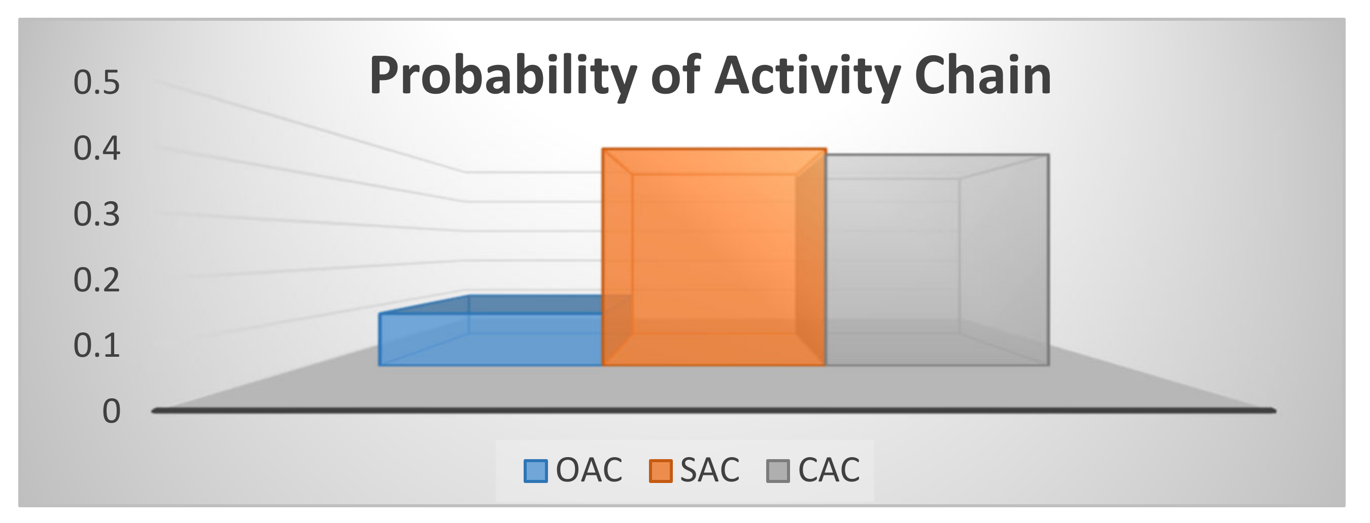
5.5.1. Estimation of Probability of Activity Chain by Using NL Model

As can be seen from Figure 3, using the NL model to estimate the probability value of the open chains, simple chains and complex chains, the results show that the probability value of simple chains is greater than open chains, but it is approximately equal to the probability value of complex chains. This result reflects the travellers’ tendency to perform daily activity with simple activity more than other chains.

In Figure 4, by using the NL model to estimate the probability value of the activity chains, the results show that the probability value of simple subsistence chains and simple maintenance chains is greater than other chains.

The probability results are shown in Figure 5; the nested logit model based on the utility function has used to estimate the probability value of the open activity chains, simple activity chains and complex activity chains; the results show that the probability value of simple subsistence activity chain (SSAC), simple maintenance activity chain (SMAC) and complex discretionary activity chain (CSAC) is greater than other chains.

5.5.2. Estimation of Utility Value by the NL Model

The NL model uses a utility function as the objective function to choose an activity chain that has a high utility, then estimates the impact of the model variables on the activity chains. The model is calculated based on the observed one-day daily activity travelling in conventional travel datasets. In this study, the chosen set of alternatives has been determined regarding observed travel parameters and travellers’ characteristics included in the dataset. The chosen set comprises nine representative activity chains: OSAC, OMAC, ODAC, SSAC, SMAC, SDAC, CSAC, CMAC and CDAC. The following variables are used for utility function: travel time, travel cost, trip distance, activity purpose, household income and household size, etc. So, we can derive utility as a function between these variables and the activity chain choice alternatives. Additionally, we used this model to identify the relationships among these sets of variables to use the model to investigate interrelationships among activity chain choice and these characteristics.

The proposed model is summarized as follows: firstly, the model has the behaviour implication as travellers make activity chain choices based on a utility model and an NL model. Secondly, it identifies the variables which have a strong effect and have high correlations with the activity chain choice by using the NL model within the utility function.

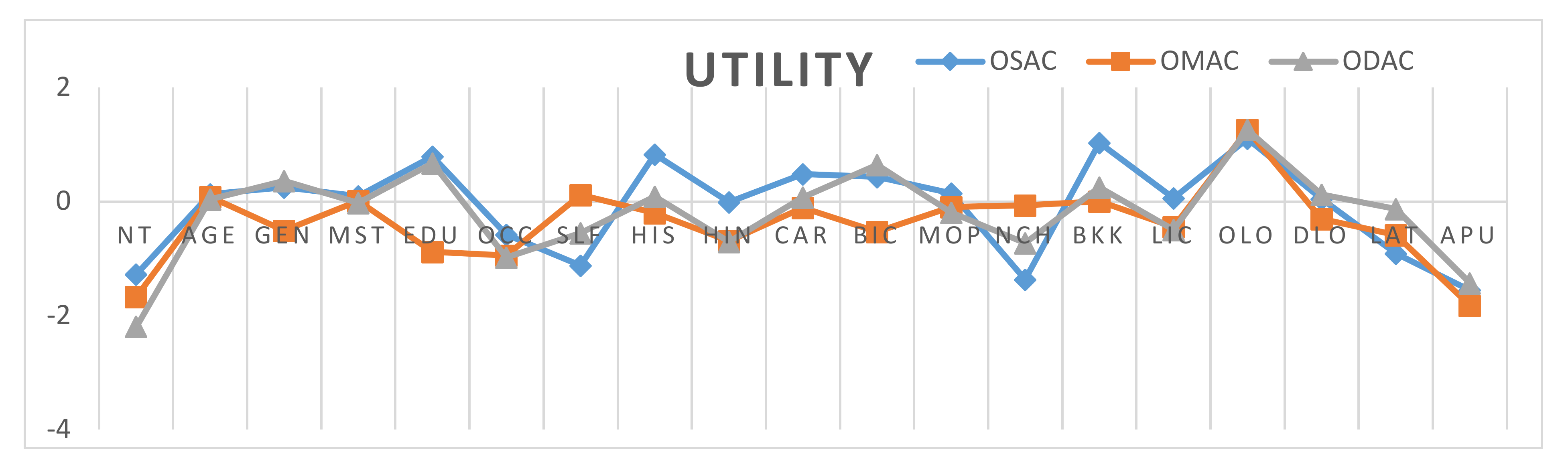
• Figure 6 presents the utility values of activity chain choice concerning the OSAC, OMAC and ODAC. According to the results, the utility values of origin location and activity purpose are greater than other parameters.
• Figure 7 describes the utility values of activity chain choice concerning the SSAC, SMAC and SDAC. According to the results, the utility values of occupation, origin location and location attribute are more significant than other parameters; therefore, these variables had a high impact on the activity chain chosen. This is consistent with the results of Arentze and Timmermans [22].
• The individual characteristics, household characteristics, travel characteristics, and location characteristics influenced the utility values concerning the travel activity chain choice. Figure 8 presents the utility values of the activity chain choice of the CSAC and CMAC. As shown, the utility values by household income, origin location, and car ownership were more affected than other parameters. This is not consistent with the results of Arentze and Timmermans [22].

5.6. The Generalized Nested Logit Model Results and Discussion of Findings

In the third analysis, the generalized nested logit (GNL) model was used to identify the influence of the different variables on the activity chain choice and estimate the coefficients of the parameters related to the complex activity chain choice. The CSAC involved the complex to discretionary activity chain (H-S/M-D-H), complex from discretionary activity chain (H-D-S/M-H), complex at discretionary activity chain (H-D-S/M-D-H), complex to subsistence activity chain (H-M/D-S-H), complex from subsistence activity chain (H-S-M/D-H), complex at subsistence activity chain (H-S-M/D-S-H), complex to maintenance activity chain (H-S/D-M-H), complex from maintenance activity chain (H-M-S/D-H) and complex at maintenance activity chain (H-M-S/D-M-H). However, some complex chains are very few in number, and missing data about these chains lead to exclusion from the analysis [69,70].

This paper applies the GNL model to estimate the interrelationships between the different characteristics (variables) and complex activity chain choice to analyse Budapest’s daily activity. The generalized nested logit model (GNL) model is calibrated by using the dataset. The result obtained by the GNL model is presented in

Table 8. Estimation coefficients and t-test of the variables of GNL.

Parameters Estimation
Variables	HSMH		HSDH		HSMSH		HMSH
	Coeff.	t-test	Coeff.	t-test	Coeff.	t-test	Coeff.	t-test
Travel time	−0.041 (−2.75)
Trip distance	3.565 (4.21)
Travel cost	−0.001 (−3.19)
Activity duration	2.419 (1.88)
Number of interchanges	0.559	1.11	−0.248	−7.45	0.195	2.37	−0.328	−4.60
Age	−0.022	−5.85	−0.019	−2.72	−0.024	−0.92	−0.017	−1.65
Gender	−0.269	−3.39	−1.238	−1.62	−1.232	−1.63	−0.751	−1.04
Marital status	0.348	8.49	0.729	3.87	0.751	1.01	2.136	8.29
Education	0.130	3.40	−0.225	−4.66	0.192	8.58	0.046	3.14
Occupation	0.609	1.13	0.111	2.57	0.099	3.52	0.249	1.35
Standard of living	−0.202	−4.72	−0.163	−0.55	−0.054	−4.20	−0.124	−0.43
Household size	0.421	1.12	0.731	1.90	0.072	2.18	0.757	4.48
Household income	0.923	3.65	1.748	3.13	−0.640	−1.87	−0.481	−1.41
Car ownership	0.774	1.24	0.423	5.75	0.420	0.77	0.696	5.28
Bike ownership	−1.733	−1.04	0.253	2.35	−0.589	−0.83	−1.038	−1.38
Moped ownership	0.705	3.67	−1.483	−3.25	−0.629	6.21	1.138	5.37
Number of children	−1.008	−1.85	−0.749	−1.46	−0.510	−1.09	−0.668	−1.39
Ticket availability	−0.020	−7.05	0.261	0.70	0.066	5.18	0.100	6.28
Driving license	0.409	5.55	−0.338	−5.46	0.322	3.43	0.210	2.29
Origin location	0.341	3.51	0.781	3.26	0.483	4.71	0.115	7.18
Destination location	0.672	1.53	1.407	8.61	−0.904	−2.67	−0.858	−4.08
Location attribute	0.850	5.72	0.728	6.07	0.675	1.16	1.237	6.85
Activity purpose	1.150	4.01	0.856	4.81	0.044	7.04	0.824	5.11
Variables	HMDH		HMSMH		HDSH		HDMH
	Coeff.	t-test	Coeff.	t-test	Coeff.	t-test	Coeff.	t-test
Travel time	−0.041 (−2.75)
Trip distance	3.565 (4.21)
Travel cost	−0.001 (−3.19)
Activity duration	2.419 (1.88)
Number of interchanges	−0.623	−1.01	−0.086	−5.16	−0.209	−2.209	−1.084	−1.57
Age	0.001	7.04	−0.005	−1.20	−0.021	−7.021	−0.026	−2.88
Gender	−0.817	−1.05	−1.451	−1.82	−0.745	−3.300	−0.589	−5.74
Marital status	0.787	4.75	0.221	6.52	0.978	4.978	0.997	1.16
Education	−0.905	1.58	0.015	4.04	0.300	1.022	−0.013	−7.04
Occupation	0.505	5.02	0.269	1.42	0.783	1.139	−0.107	−3.46
Standard of living	−0.219	−2.69	−0.046	−7.16	−0.022	−6.574	−0.059	−1.19
Household size	0.338	4.84	0.426	1.09	−0.139	−2.388	−0.176	−3.39
Household income	−0.646	−1.80	−0.191	−3.54	1.396	−1.285	0.115	4.28
Car ownership	−0.092	−6.16	−0.096	−8.17	−0.574	−6.252	−0.067	−1.11
Bike ownership	−0.951	−1.19	−0.895	−1.18	0.388	0.981	−1.204	−1.42
Moped ownership	0.443	3.46	0.828	3.51	−1.175	−2.881	0.356	3.71
Number of children	−0.556	−1.59	−0.877	−1.61	−0.285	−1.558	−0.224	−2.11
Ticket availability	−0.150	−2.38	−0.180	−3.47	0.252	6.157	0.008	1.02
Driving license	0.024	4.03	−0.167	−4.22	0.926	8.585	−0.525	−5.64
Origin location	0.914	9.55	0.585	3.21	−0.981	−1.160	−0.233	−6.44
Destination location	−0.198	−1.88	0.897	6.08	0.881	1.571	1.161	3.21
Location attribute	0.601	4.49	0.152	1.68	3.630	2.331	0.707	5.08
Activity urpose	0.502	3.10	1.419	8.74	1.558	4.059	0.505	3.88

. Different nesting structures have been implemented to carry out the activity choice analysis. Estimating the generalized nested logit model has been most generally undertaken by limited information and maximum likelihood techniques. This method first estimates the correlation of parameters for the generalized nested and then calculates the parameters’ coefficient for each activity chain based on the log sum values’ computation.

The significance of variables is checked, and the non-significant variables are eliminated based on logical signs and t-statistic. As a result, the overall model fit is adequate. It is also observed that most of the variables have a good coefficient value, which indicates the importance of these variables in the model. The parameter coefficients for the generalized nested logit model are presented in Table 8.

• For the complex from subsistence activity chain (H-S-M-H), the activity purpose, household income, location attribute, and car ownership have a positive effect on the (H-S-M-H). In contrast, bike ownership has a negative and slight impact on the (H-S-M-H). However, the activity purpose has a more significant influence on the (H-S-M-H). This is consistent with the results of Primerano et al. [37].
• For the complex from subsistence chain (H-S-D-H), the results show that household income, destination location, activity purpose and origin location positively affect the (H-S-D-H). In contrast, moped ownership has a negative and slight impact on the (H-S-D-H). However, household income has a more considerable influence on the (H-S-D-H) compared to other variables. According to the result, the household income has a significant impact on the complex activity chains. This finding matches that of Valiquette and Morency [15].
• According to the results for the complex at subsistence activity chain (H-S-M-S-H), the marital status has a more considerable influence on the (H-S-M-S-H) than other variables. At the same time, location attributes, origin location and car ownership positively affect the (H-S-M-S-H). In contrast, gender has a negative and slight impact on (H-S-M-S-H). This is consistent with the findings of Ahmed and Hani [1].
• For the complex from maintenance activity chain (H-M-S-H), the result has been found that the marital status, location attribute, activity purpose and household size positively affect the (H-M-S-H). However, the marital status has a higher impact on the (H-M-S-H) compared to other variables. So, this result proves the marital status is a necessary variable to designate complex activity chains [11].
• For the complex from maintenance chain (H-M-D-H), the results indicated that origin location, marital status and location attribute positively impact the (H-M-D-H). In contrast, education has a negative and slight effect on the (H-M-D-H). So, origin location has a more considerable influence on the (H-M-D-H). This result reinforces that the origin location is vital to specify the complex chains.
• According to the results for the complex at maintenance chain (H-M-S-M-H), the activity purpose has a greater effect on the (H-M-S-M-H) than other variables, while destination location and household size positively affect the (H-M-S-M-H). In contrast, gender has a negative and slight impact on (H-M-S-M-H). This result confirms that the activity purpose is essential to assign the complex activity chains.
• For the complex from discretionary chain (H-D-S-H), the results found that location attribute, activity purpose, and marital status have a positive effect on the (H-D-S-H). In contrast, moped ownership has a lower impact on (H-D-S-H). However, location attribute has a greater effect on the (H-D-S-H) compared to other variables.
• For the complex from discretionary activity chain (H-D-M-H), the results show that the destination location, marital status, location attribute, and activity purpose positively affect the (H-D-M-H). However, the destination location has a more significant influence on the (H-D-M-H) than other variables.

In summary, according to the results from the GNL model, when travellers or household members planned to perform complex activity chains, they take into account the following variables: the activity purpose, location attribute of destination, origin location, and marital status in order to obtain a high utility from the chain and because these variables have an increased effect on the complex chains.

5.6.1. Estimation of Probability of Complex Activity Chain by Using GNL Model

Figure 9 shows the results of using the GNL model to estimate the probability value of the complex maintenance chain, complex subsistence chain, and complex discretionary chain. The results show that the probability value of complex subsistence chains is greater than other chains. This result reflects travellers’ tendency to perform one activity more besides the subsistence activity within a chain.

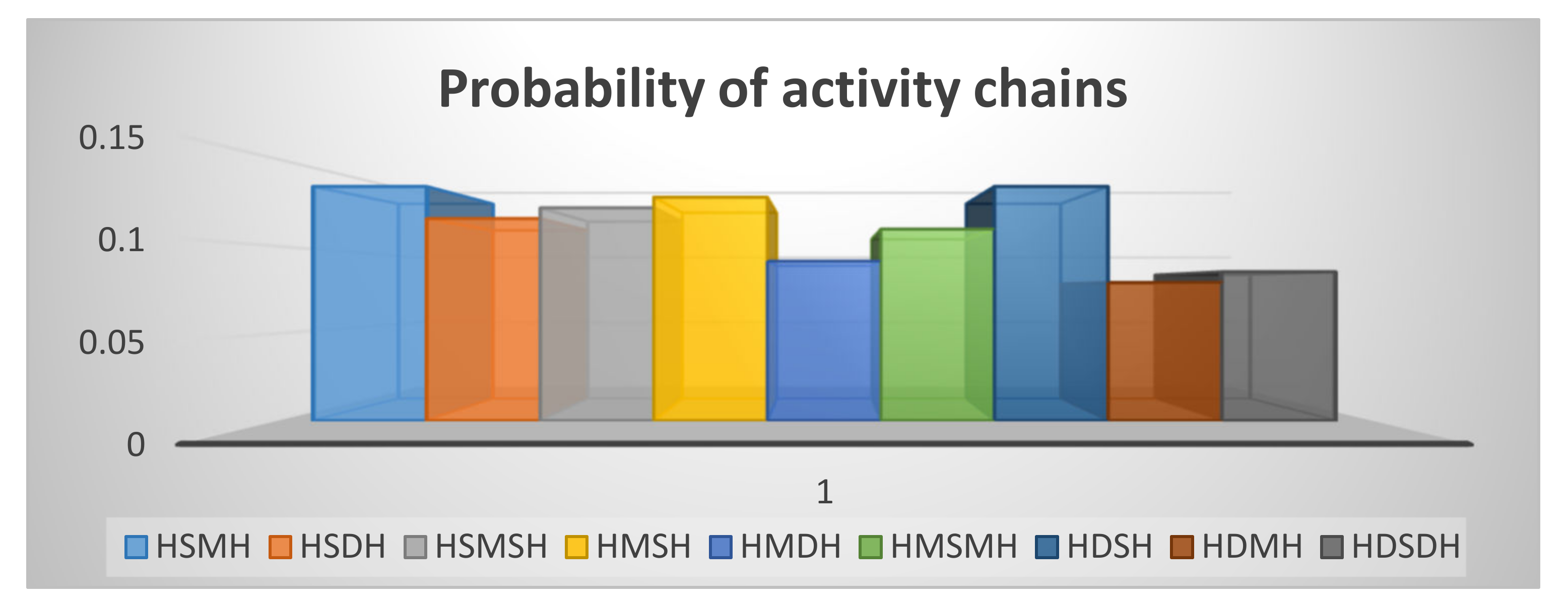
According to the results shown in Figure 10, by using the GNL model to estimate the probability value of the complex chains, the results showed that the probability value of complex from subsistence chains (HSMH), complex from maintenance chains (HMSH) and complex from discretionary chains (HDSH) is greater than other chains. This result confirms travellers’ tendency to perform one activity more (subsistence or maintenance or discretionary) within the complex subsistence activity chains and to obtain more benefit (utility) from the daily activity chain.

According to the results shown in Figure 11, the GNL model based on the utility function has been used to estimate the probability value of the complex activity chains; the results showed that the probability value of complex from subsistence chains (HSMH), complex from maintenance activity chains (HMSH) and complex from discretionary activity chains (HDSH) is greater than other chains. This result reflects the household members’ tendency to achieve more than one activity (subsistence or maintenance or discretionary) within the complex subsistence chains and to obtain more utility from the daily activity chain.

5.6.2. Estimation of Utility Value by the GNL Model

The GNL model is with a utility function as the objective function to choose a complex activity chain that has a high utility, then it estimates the impact of the model variables on the activity chains. The model is calculated based on the observed daily activity travelling. In this paper, the chosen set of alternatives has been dependent on practical travel parameters and travellers’ characteristics included in the dataset. A choice set comprised nine representative complex activity chains: HSMH, HSDH, HSMSH, HMSH, HMDH, HMSMH, HDSH, HDMH and HDSDH. The following variables are used for utility function: age, activity duration and location characteristics, etc. So, we can derive utility as a function between these variables and the complex chain to choose alternatives.

The proposed model is as follows: Firstly, the model has a behaviour implication as travellers make complex activity chain choices based on a utility model and a discrete choice model. Secondly, it identifies the variables which have a high impact on the complex chain choice by using (GNL) model within the utility function. Thirdly, it investigates interrelationships among complex chain choice and these sets of variables.

• Individual, household, travel, and location factors influenced the utility values concerning the complex activity chain choice. Figure 12 presents the utility values of the complex activity chain choice of the HSMH, HSDH and HSMSH. As shown, the utility values by household income, origin location (home location), location attribute, activity purpose and car ownership have more impact than other parameters. The results match that of Zohreh et al. [19].
• Figure 13 presents the utility values of complex activity chain choice concerning the HMSH, HMDH and HMSMH. According to the results, the utility values of marital status, origin location (home location), location attribute and activity purpose are greater than other parameters, so that the home location and activity purpose have a stronger effect on the complex activity chain choice.
• The results of the GNL model are shown in Figure 14, which describes the utility values of activity chain choice concerning the HDSH and HDMH. According to the results, the utility values of marital status, location attribute of the destination and activity purpose are more significant than other parameters; therefore, these variables had a strong effect on the activity chain chosen.

6. Conclusions

The conceptual deficiencies of the conventional trip-based models that use individual trips as the unit of analysis led to the emergence of the activity chain model. The activity-based model has been used to provide a better theoretical underpinning of travel behaviour research as it addresses why people travel and how decisions regarding trips are made. According to that, analysis and modelling of travellers’ behaviour concerning the activity chain are essential for analysing existing transportation systems and for policy testing and effective planning of future transport networks. Therefore, this study examined the relationships among activity chains and other variables which involved individual characteristics, household characteristics, location-related characteristics, travel-related characteristics and activity characteristics. To achieve this work, we used a multinomial logit model, nested logit model, and generalized nested logit to analyse these relationships. This paper proposed a typology of activity chains based on past research and a collected dataset to conduct this analysis. Further, this paper presents a rigorous analysis of the wide range of characteristics contained within 24 variables and their influence on activity chains.

The analysis undertaken aims to identify the relationships between the activity chain behaviour of travellers with different factors by using logit models based on the utility function. The model contained a wide range of variables that affect activity chains in order to obtain the maximum utility from the activity chain choice for a thorough understanding of the activity chain behaviour of travellers in Budapest city.

Further, the activity chain choice model is formulated using various structures to understand the activity chain behaviour.

The most explanatory variables have been directly determined from the data based on a household survey of travellers in Budapest. However, trip data have also been defined, such as trip distance and travel cost computed from the highway transit network and the GIS database. Thus, a number of significant variables are included in the utility function consisting of the activity chain.

Moreover, the utility function presented in this study highlights the concepts of utility maximization through performing the daily activity of travellers. This function includes the utility of performing daily activities so that it introduces a trade-off between different chains based on utility. This model allows for accommodating travel activity chain selection depending on individual and household characteristics, travel characteristics and location characteristics to achieve the best personal utility. New terms in the utility function are introduced to improve model performance and simplify estimating the maximum utility of activity chain selection.

In the model specification, all the estimated parameters have expected signs with apparent magnitudes. They are found to be significant at the (0.05) confidence level in explaining trip chaining behaviour in Budapest city. Additionally, we have reviewed the estimates of the variables and interpreted these estimates focusing on the variables that have high significance on the activity chains. The coefficients and t-tests of variables showed that all explanatory variables were significant. Still, the effects and contributions of each variable were not the same, so they were sorted according to their impact on the model. According to that, the results found:

• The analysis and modelling using the MNL of the open activity chain, simple activity chain and complex activity chain shows that the occupation, household income, location attribute, activity duration and activity purpose have a strong effect on the activity chains. So, these variables are considered when the travellers assign their daily activity chains;
• The analysis and modelling using the NL model of different types of activity chains shows that the traveller identifies their chain choice depending on the origin location, activity duration, activity purpose, location attribute and activity duration. At the same time, these variables have a high impact on the activity chains;
• The analysis and modelling using a generalized nested logit (GNL) of the different types of complex chains confirm that the activity purpose, location attribute origin location, marital status, trip distance, and activity duration significantly influence the activity chains. So, these variables are weighed when the travellers select the complex activity chains.

Several conclusions regarding the research in this paper on activity-based modelling can be drawn:

• Although the activity-chain-modelling structures are evolving rapidly, it is already possible to summarize these models’ essential new structural features. Among them is the explicit incorporation of intra-household interactions.
• The activity chain model used in this study is based on the detailed classification of activities and travel segmentation. In particular, activities are grouped by type (subsistence, maintenance, discretionary) and setting (open, simple, complex), where a special modelling technique is applied for each particular type.
• The skeleton of the activity chain model can be outlined as a sequence of conditional choices that include level of decision making, chain level, and trip level.
• The analytical structure of the new generation of activity-based models in the application is fundamentally different from the conventional aggregate models, which depended on the tour-based models. Instead of fractional–probability calculations at the origin–destination pairs of zones, the model is applied at the level of the individual, households, and tours, with no explicit constraints on the number of variables or population/travel segments.
• The experiences of developing and applying the activity chain models have revealed some challenging issues that should be addressed in future research. These include a better linkage between the activity scheduling and travel decision-making stages, incorporation of activity-chains duration models, and many others.

Although many of the concerns and scepticism involved in moving to the activity chain models of travel demand models can be addressed by better explanation and practical demonstration of the advantages of the new models, the following issues, in our view, can be classified as valid concerns that need to be addressed by future research to accelerate the widespread application of activity-based models in practice:

• The complexity of activity-based models and the larger number of interacting model components make it difficult to trace the model’s sensitivity to input factors in an analytical sense. However, more work can be done to better understand and describe the output of the activity-based model system framework from the analytical point of view and the development of built-in software features for tracking the decisions of sample households and persons between alternatives.
• The purpose of a realistic description of travel behaviour and the complex structure of activity chains will lead in future to many researchers understanding the analytical framework of the activity-based models, which should be extended to incorporate various decision-making rules within households and mechanisms of performing trip chaining. Furthermore, this framework will open the way to explicitly modelling interactions between participating agents (persons, households, firms) on an individual basis and aggregating behaviour patterns.

Further progress in moving from tour-based to activity-based modelling approaches depends upon successfully addressing these issues in the future. In addition, it will require constructive communication and cooperation among modellers, researchers, practitioners, and ultimately, regulators.