Article

Risk Assessment and Prediction of Air Pollution Disasters in Four Chinese Regions

School of Management, Henan University of Science and Technology, Luoyang 471023, China
*
Author to whom correspondence should be addressed.
Sustainability 2022, 14(5), 3106; https://doi.org/10.3390/su14053106
Submission received: 4 February 2022 / Revised: 2 March 2022 / Accepted: 3 March 2022 / Published: 7 March 2022
(This article belongs to the Topic Climate Change and Environmental Sustainability)

Abstract

:
Evaluating the regional trends of air pollution disaster risk in areas of heavy industry and economically developed cities is vital for regional sustainable development. Until now, previous studies have mainly adopted a traditional weighted comprehensive evaluation method to analyze the air pollution disaster risk. This research has integrated principal component analysis (PCA), a genetic algorithm (GA) and a backpropagation (BP) neural network to evaluate the regional disaster risk. Hazard risk, hazard-laden environment sensitivity, hazard-bearing body vulnerability and disaster resilience were used to measure the degree of disaster risk. The main findings were: (1) the air pollution disaster risk index of Liaoning Province, Beijing, Shanghai and Guangdong Province increased year by year from 2010 to 2019; (2) the mean absolute error (MAE), root mean square error (RMSE) and mean absolute percentage error (MAPE) of each regional air pollution disaster risk index in 2019, as predicted by the PCA-GA-BP neural network, were 0.607, 0.317 and 20.3%, respectively; (3) the predicted results were more accurate than those using a PCA-BP neural network, GA-BP neural network, traditional BP neural network, support vector regression (SVR) or extreme gradient boosting (XGBoost), which verified that machine learning could be used as a method of air pollution disaster risk assessment to a considerable extent.

1. Introduction

With the proliferation of high-intensity human engineering activities on a global scale, the global air pollution trend has become more and more obvious [1,2,3]. Extreme weather events frequently occur and have caused a series of disasters, and a high degree of air pollution seriously endangers human health [4,5,6,7,8]. High concentrations of PM2.5 and PM10 have significantly increased population mortality [9,10]. According to the Global Burden of Disease (GBD) report, nearly 4.09 million people died as a consequence of outdoor air pollution in 2016 [11,12]. The Environmental Law and Policy Center of Yale University published China’s environmental quality ranking in the Global Environmental Performance Index Report 2018, ranking it 120th among 180 countries and regions in the world. China’s overall assessments of PM2.5, nitrides and sulfides were ranked 177th, and the air quality compliance rate of 338 cities across the country was 35.8%. Among all the kinds of air pollution, the impacts of PM2.5, PM10, and nitrides and sulfides on human health have become a research focus worldwide. Many studies have shown that the population mortality rate and the incidence of various human respiratory and circulatory system diseases are closely related to short-term exposure to air pollution [13,14,15,16,17,18,19,20]. Burkart et al. [21] adopted bivariate response surface models (BRSMs) and generalized additive models (GAMs) to assess the increased mortality risk from high temperatures and air pollution. Willers et al. [22] designed a case-crossover method to analyze the associations among mortality, temperature, and air pollution and found significant synergistic effects from high temperature and air pollution on mortality. Requia et al. [23] applied the integrated exposure-response function (IERF) to estimate the influence of PM2.5 on premature mortality, which found that reducing traffic congestion and land using efficiency could reduce air pollution and population mortality. Zhao et al. [24] utilized statistical data to evaluate the influence of O3 and PM10 on the risk of depression or anxiety diagnosis in the general population. Liu et al. [25] studied the substantial association between the psychological wellbeing of citizens in various aspects and air pollution. Yuan et al. [26] evaluated the impact of air pollution and green spaces on people’s subjective well-being (SWB) in China.
With the rapid development of the national economy and the advancement of industrialization and urbanization, the overall air quality in China has deteriorated significantly, and extreme air pollution incidents have occurred frequently [27,28,29,30,31,32]. To date, existing studies have carried out a comprehensive air pollution disaster risk assessment regarding the economy, society and ecology. Sun et al. [33] evaluated the gestational exposure to air pollution of 6275 pregnant mothers in Zhejiang Province in China in 2013–2017. Du et al. [34] studied indoor and outdoor polycyclic aromatic hydrocarbons (PAHs) and population inhalation exposure in two rural counties in Shanxi and Guizhou provinces. Zhang et al. [35] analyzed air mass transportation and the sources of volatile halogenated hydrocarbons (VHCs) in Beijing, to better understand the health risks of VHCs. Bao et al. [36] analyzed the pollution characteristics, atmospheric photochemical reactivity, human health risk and sources of carbonyls during a heavy air pollution episode in Chengdu in China. As for the weighting methods, some researchers have adopted the analytical hierarchy process (AHP), the fuzzy analytical hierarchy process (FAHP), the Delphi method, the entropy method (EM), and so on to evaluate the association among economic development, air pollution, and people’s health [37,38,39,40]. With the continuous improvement of information technology, some researchers have used machine learning tools to effectively assess the air pollution disaster risk. Du et al. [41] used the length-changeable incremental extreme learning machine (ELM) to forecast air quality information, which is essential for controlling and managing air pollution. Li et al. [42] adopted a backpropagation (BP) neural network to simulate air pollution control in the future, objectively and effectively evaluating the performance of air pollution. However, the BP model will make its prediction error fall into the local minimum of the error space, resulting in low convergence speed and affecting the prediction’s accuracy. A genetic algorithm (GA) with good optimization ability could improve the search performance of the BP neural network; the GA-BP neural network had better predictive performance in the modeling of machine learning [43].
Based on the above literature review and the disaster risk theory, to further improve the assessment indicators, we first considered the natural environment, economic and social development, population, residents’ health status, and the death rate from diseases as air pollution disaster risk assessment indicators. Then, we constructed an air pollution disaster risk assessment indicator system from hazard risk, hazard-laden environment sensitivity, hazard-bearing body vulnerability and disaster resilience. Finally, the authors introduced principal component analysis (PCA) to analyze the constituent indicators of air pollution disaster risk in Liaoning Province, Beijing, Shanghai and Guangdong Province, to acquire the training data for the GA-BP neural network. This research has been divided into four sections. The first section will introduce the background of the research. The materials and methods section will introduce the study area, data sources, indicator system and the principle of the PCA-GA-BP neural network. The analytical results section will introduce the air pollution disaster risk index and the changing trends of the risk index, as displayed by GIS technology from 2010 to 2019. The final section will offer a discussion, our conclusions, and the limitations of this research.

2. Materials and Methods

2.1. Data

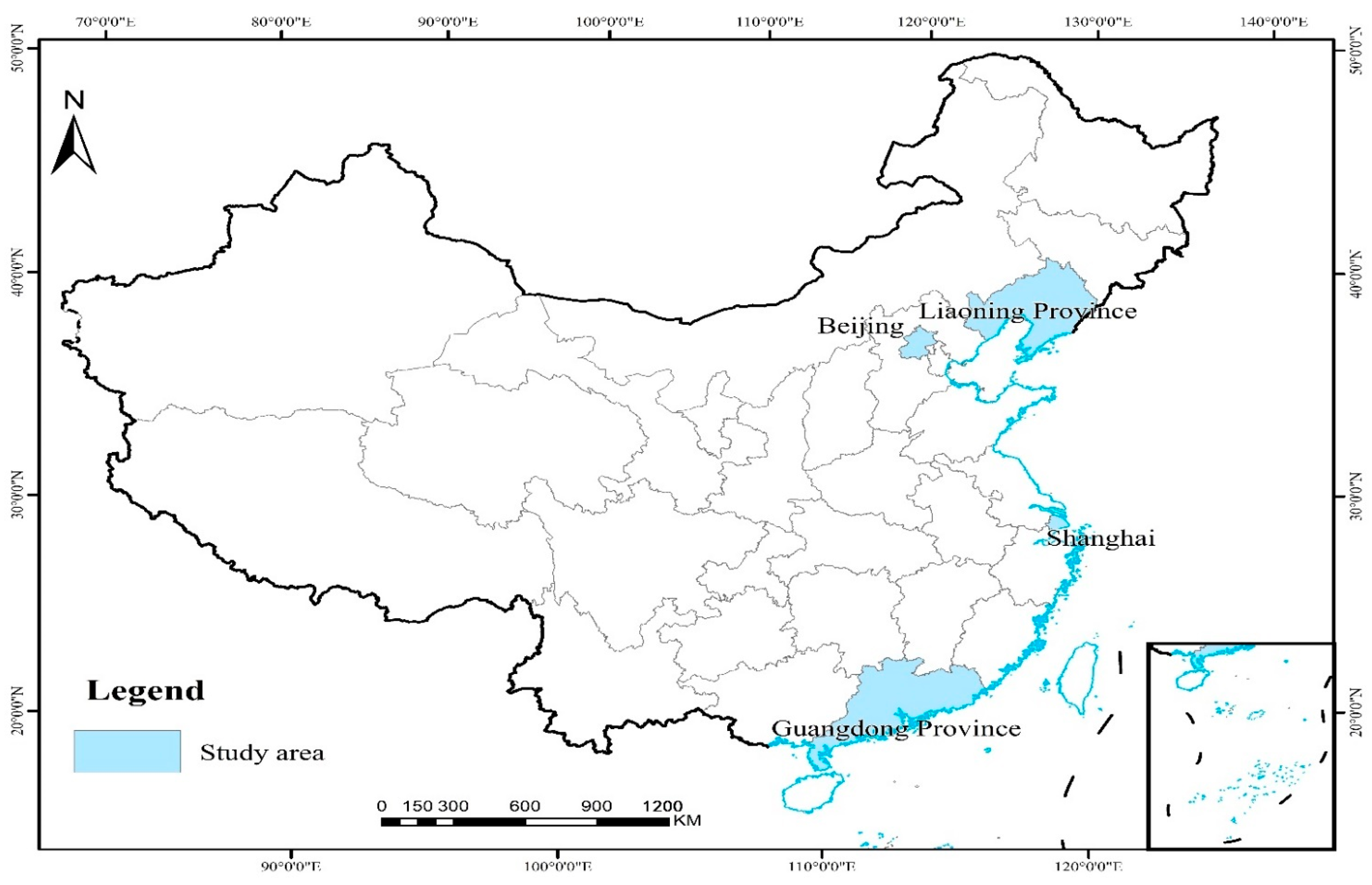
2.1.1. Overview of the Study Area

In order to verify the science and rationality of the method, Liaoning Province, Beijing, Shanghai and Guangdong Province were used as examples to carry out the applied research. Liaoning Province is located in the southern part of northeast China, and it is bounded by latitude 38°43′–43°26′ N and longitude 118°53′–125°46′ E, with a total area of 148,600 square kilometers. Beijing is located in the northern part of China with a total area of 16,400 square kilometers, between latitude 39°26′–41°03′ N and longitude 115°25′–117°30′ E, at the junction of the North China plain, the Taihang Mountain and the Yanshan Mountain. Shanghai is located in the middle of the eastern coast of China, between latitude 30°40′–31°53′ N and longitude 120°52′–122°12′ E. It is the center point between China’s north and south coasts, with a total area of 6300 square kilometers. Guangdong Province is located in the most southern part of China′s mainland, between latitude 20°13′–25°31′ N and longitude 109°39′–117°19′ E. The total land area of the province is 179,800 square kilometers, which is about 1.87% of the country’s landmass. The characteristics of heavy industrial structures in the northeast region have been prominent for many years, and the development of heavy industry still puts great stress on the ecological environment. In 2015, the total emissions of industrial-source SO2 from the three northeastern provinces reached 1,452,400 tons; this was about 81.2% of the total emissions of SO2 in the region. Liaoning Province was an important industrial area, with more value to research for carrying out risk assessments of dangerous air pollution levels. Pollution emissions had an impact on both the birth rate and the death rate. This effect was mainly reflected in the more developed coastal and inland central cities in China. The agglomerations of Beijing, Shanghai and Guangzhou Province were selected to better analyze the changing trends of China’s regional air pollution disaster risk. The geographic locations of the study areas are shown in Figure 1.

2.1.2. Details of the Data Sources

The data on regional economic and social development used in this study includes regional GDP, the density of economic activity, the proportion of secondary industry, building construction areas, urban green space areas, health expenditure, energy conservation and environmental protection expenditure, population status, and so on. The data regarding residents’ health status included birth rate, death rate, natural growth rate, the death rate from individual diseases, average medical treatment visits and average annual hospitalization rate. The meteorological data included annual average temperature, relative humidity and rainfall data. The above data range was from 1 January 2010 to 31 December 2019 and was sourced from the National Statistics Administration, the China City Statistical Yearbook and China Health Statistical Yearbook. The annual average PM10, PM2.5, SO2, NO2, O3 and CO were calculated from the daily data, which were from the US Embassy’s Air Quality Report (https://www.airnow.gov/ accessed on 25 October 2021) and the National Statistics Administration. In this research, using a PyCharm environment in Python and other tools, the six pollutant concentrations are shown in Figure 2a–d. The standard deviations of the annual average of the six major pollutant concentrations in each region from 2010 to 2019 are shown in Table 1.
The annual average concentrations of SO2, PM10, CO and PM2.5 of Liaoning province, Beijing, Shanghai, and Guangdong Province have decreased year by year from 2010 to 2019. However, the annual average concentrations of NO2 in each region have not decreased significantly. The annual average concentrations of O3 in each region have increased yearly. The transport effect of air pollution, photochemical decomposition and human activities had a significant impact on increasing the concentration of O3. Related studies conducted in other regions also showed that the concentrations of O3 were negatively associated with the concentrations of SO2, NO2, PM10, CO and PM2.5 [44,45,46,47].

2.1.3. Construction of the Indicators System

The regional assessment index system of air pollution disaster risk constructed from the perspective of four aspects is shown in Table 2.
Based on the theory of disaster risk systems and the existing related research results, considering the current situation regarding air pollution and the availability of data, this study has constructed an indicator system of air pollution disaster risk assessment from hazard factors, hazard-laden environments, hazard-bearing body vulnerability, and disaster resilience. The hazard factors were directly responsible for air pollution disasters. Previously published studies have shown that the major six air pollutants affected the residents’ health. Therefore, the annual average concentrations of SO2, NO2, PM10, CO, O3 and PM2.5 were used as directly influencing indicators of regional air pollution. Hazard-laden environments include the natural environment and human environments. The occurrence of air pollution disasters is closely related to the regional natural environment and to economic and social development. Higher emissions of industrial and residential pollutants caused higher average annual temperatures. The average annual air humidity and the average annual rainfall decreased the possibility of human exposure to air pollution. The more developed regions consumed more energy and released more toxic gases and particulate matter, which increased their risk of air pollution. With their higher proportions of secondary industry, the degree of air pollution and damage and the sensitivity of hazard-laden environments would be higher. Construction dust was also a major source of inhalable particulate matter; therefore, the more building construction took place in an area, the higher the concentration of inhalable particulate matter. In addition, this article selects the levels of regional population birth rate, death rate, and the death rate from specific diseases to evaluate the sensitivity of air pollution disaster risk. Therefore, this research selected the natural environment, economy, population, and residents’ health to quantitatively evaluate the sensitivity of regional hazard-laden environments. Hazard-bearing body vulnerability was adversely influenced by disasters. Many developed regions are predominantly urban areas. The higher density of the regional population and the high proportion of the population living in urban areas causes more people to suffer from air pollution problems and increases the level of hazard-bearing body vulnerability. Existing related studies have shown that urban green vegetation could absorb harmful gases and construction dust, which could decrease the danger of air pollution and the population’s vulnerability to its hazards. Therefore, this research selected a regional population, a proportion of the urban population, a densely populated area, and urban green spaces to evaluate the body’s vulnerability to this hazard. Disaster resistance represents the ability to overcome air pollution issues. This research mainly considered the resilience of the whole region and individuals regarding air pollution adverse events. On the one hand, with higher regional health expenditure and energy conservation and environmental protection expenditure, a greater number of medical insurance participants and health workers could increase a region’s ability to deal with air pollution and decrease the air pollution disaster risk. On the other hand, higher per capita disposable income and per capita consumption expenditure could increase the residents’ ability to prevent and deal with air pollution adverse events. Therefore, the six indicators listed above are selected as the evaluation indicators of regional disaster resilience.

2.2. The Principle of the PCA-GA-BP Neural Network

The BP neural network used in the study, comprising an input layer, hidden layer and output layer, was a multilayer feedforward neural network with backpropagation, which was trained by supervised learning and could handle complex nonlinear mapping relationships [48]. It had the characteristics of signal forward propagation and error backpropagation. Each layer of the BP neural network contained 1 or n neuron nodes. The data first entered the network through the input layer, was processed by the hidden layer, then transmitted to the output layer, and finally, processed and output by the output layer. If there was a large error between the output value and the expected value, the error data would propagate back along the original path, adjust the network weight and threshold, and repeat the above operations until the error reached the allowable threshold or the maximum number of iterations of the algorithm. The steepest descent method in the BP neural network framework was to minimize the error between the output value and expected value. However, it was difficult to find an optimal global solution because of its function and the randomness of setting the initial weight and threshold. In this research, a GA was imported to enhance the stability and efficiency when searching for the optimal global solution [49]. It is worth noting that there are many influencing factors in air pollution adverse events. Dimension reduction was vital to the accuracy of the model because of the strong coupling and redundancy in the indicator system. PCA was able to merge the original features and reduce the dimension to simplify computation, especially aiming at strong linear indicators [50,51]. When the data were processed by PCA, only some principal influencing factors were considered. In order to obtain more accurate prediction results, this research adopted a GA-BP neural network to predicate the training data processed by PCA.

2.2.1. Data Standardization

Data standardization could improve the learning efficiency and prediction accuracy of the GA-BP neural network. The data were standardized to the same range, such that [0, 1], which means that the data dimension was unified. The original data obtained, according to the regional risk assessment indicators in Table 2, had positive and negative effects. At the same time, due to the inconsistency of the data units, the data needed to be standardized to eliminate the dimensional impact. Positive impact indicators were treated as Equation (1) and negative impact indicators were treated as Equation (2). Data were standardized as follows:
X = X i j X ¯ J S J
X = X i j X ¯ J S J
where X* is the standardized data, X i j represents the real value of the index of the sample, X ¯ J represents the mean value of the index, S J represents the variance of the index.

2.2.2. PCA Principle

When modeling multivariate data, the complexity and computation time of the model may be increased by the variables. PCA is adopted to reduce the dimensions of the dataset to solve this problem. PCA can easily overcome the disadvantages of computational complexity resulting from a large number of dependent variables. The idea of using PCA was to map the n-dimensional features to k-dimensions (k < n) according to the maximum variance theory [52]. PCA is a feature-extraction method based on multivariate statistical regression. It can linearly transform data characteristics, which are comprehensive indicators containing the vast majority of the original variable parameters and are independent of each other. The essence of PCA is an orthogonal coordinate system transformation, which can reduce the dimensions of the original indicators with specific relevance and combine them to form a new set of comprehensive indicators. In data analysis, the original dataset is projected into a new space through the feature analysis of the matrix, so as to reduce the dimensions of the data. Firstly, the component with the largest variance contribution rate is selected as the first principal component. If the variance contribution rate is not high enough, the one with the second variance contribution rate is selected as the second principal component, until the cumulative variance contribution rate reaches the preset value. The variance contribution rate in this research was used as the weight of the final evaluation of regional air pollution disaster risk.

2.2.3. GA Principle

The genetic algorithm is a random searching and optimizing algorithm that evaluates each coded individual according to a self-defined fitness function and eliminates the bad fits. In addition, it selects the coded individuals with good fitness to select, cross over and mutate, and generates offspring groups several times until a coded individual approaches the optimal solution [53]. In this research, GA was applied to optimize the weight and threshold of the BP neural network. After the maximum generation of the selection operation, crossover operation, and mutation operation, the GA searches for the best-fitting value corresponding to an optimal individual as the initial weight and threshold of the BP neural network. When using a genetic algorithm to solve optimization problems, there are three coding methods for establishing optimization variables: vector form coding, binary form coding, and matrix form coding. Because the weight and threshold form the matrix function to optimize each element, the elements are first removed separately and then put into the vector, in order to complete the coding. The empirical range of the weight and threshold in this study was −1–1. The parameters of GA are selected as follows: population size is commonly set as 10–100. In this research, the population size was 55, the population evolution iteration time was 35, the crossover probability was 0.7, and the variation probability was 0.009.

2.2.4. BP Neural Network Principle

The most basic component of the neural network is the neuron, which is the basic information-processing unit of the neural network operation and consists of three basic elements: a set of connections, an adder, and an activation function. The BP neural network is a kind of typical multilayer feed-forward neural network with the ability to approximate any continuous function and nonlinear mapping. Its topological structure includes an input layer, hidden layer and output layer. Each neuron between adjacent layers is fully connected, but the neurons in the same layer have no connections. To ensure that the network matches the mapping relationship between the input and output, the BP neural network studies and adjusts the connecting weight and threshold value among neurons, according to the input and output of given samples [54]. The training process of BP neural network was shown as Figure S1.
The PCA-GA-BP neural network algorithm can be divided into four parts, mainly including data standardization, data dimension reduction using PCA, optimization using a GA algorithm, and prediction using a BP neural network. Data standardization enhances the data generalization ability of the neural network. The prediction model is based on PCA and replaces a large number of original interrelated indicators with a smaller number of uncorrelated principal indicators, to further improve prediction accuracy. Finally, the model, based on a GA-BP neural network, is ready to predict. The flow chart of the PCA-GA-BP neural network algorithm was shown in Figure S2.

3. Analytical Results of Air Pollution Disaster Risk

The 30 standardized indicators were analyzed as principal indicators. In Table A1, it can be seen that the tangency quantity of KMO sampling was 0.662 (>0.5), and the Sig value of the Bartlett spherical degree test was 0.000 (<0.05), demonstrating that the indicators were independent of each other to a certain extent and that the PCA could be used to reduce the dimensionality and feature selection of the data. According to the principle that the characteristic value was greater than 1, the first four indicators were selected as the main indicators. The variance contribution rates were 47.1%, 24.0%, 13.2% and 9.13%, respectively, and the cumulative contribution rate was 93.4%, which could basically reflect all the information in the original indicators.
The characteristic values and contribution rates of each principal component are shown in the Appendix A (Table A2). Taking the first four items as the principal component indicators of air pollution disaster risk and expressing them as P 1 , P 2 , P 3 and P 4 , the indicator loading of each principal component and the original standardized indicator was calculated as shown in Table A3 in the Appendix A. The loading values in the principal indicator loading matrix reflected the degree of importance of the role of each indicator in the air pollution disasters risk. Hence, the loading values of each indicator could be used to express the indicator weight. Using the weighting equation calculated the score of each region according to 4 principal indicators. The air pollution disaster risk index with different principal components can be expressed as:
R i =   ω j X i j
where R i is the risk index of the i t h evaluation unit with different principal indicators, X i j is standardized values of the j t h indicator of the i t h evaluation unit, and ω j is the loading value of the j t h indicator on the corresponding principal indicators.
Using the principal indicators’ contribution rates, the comprehensive score was calculated using a weighted model; the comprehensive air pollution risk index R could be expressed as in Equation (4):
R = R 1 P 1 + R 2 P 2 + R 3 P 3 + R 4 P 4   P 1 + P 2 + P 3 + P 4  
where R 1 , R 2 , R 3 and R 4 represent the risk index of each unit on each principal indicator after being calculated by Equation (3). P 1 ,   P 2 ,   P 3 and P 4   represent the corresponding contribution rate of each indicator.
As shown in Table A4 in the Appendix A, the comprehensive risk index of each region was calculated using Equations (3) and (4). The comprehensive risk index calculated from Table A4 showed that there were significant temporal and regional differences in the comprehensive air pollution disaster risk index among regions in the period from 2010 to 2019. The changing trend in the comprehensive air pollution disaster risk index is shown in Figure 3a–d over the past 10 years. Considering the changes in the human settlement environment, the health status of the population, and the death rate from various diseases, the air pollution disaster risk index showed a significant increasing trend from 2010 to 2019.
Calculating the risk index quartiles resulted in −5.832, −1.471, and 4.945, respectively, and the standard deviation was 7.512. GIS technology was used to take the quartiles and standard deviation of the comprehensive air pollution disaster risk index as references. Using the natural fracture method, the risk index levels of each region in the past 10 years were divided into five levels: lower risk (P ≤ −5.832), low risk (−5.832 < P ≤ −1.471), medium risk (−1.471 < P ≤ 4.945), high risk (4.945 < P ≤ 7.512) and higher risk (7.512 < P).
It can clearly be seen from the changing trend of the risk index of each region over the past 10 years that Guangdong Province was the area most seriously affected by air pollution, the death rate from various diseases has increased significantly year by year, and the birth rate has also shown a downward trend. Due to the positive and negative interaction of the indicators, it could be suggested that the air pollution disaster risk in the old industrial area of Liaoning Province is slowly increasing, but it presents a low risk. The extent to which Beijing and Shanghai have been affected by air pollution disasters was increasing year by year. The data showed a slowly increasing trend and indicated that the region was paying attention to the protection and governance of the environment when developing its economy. Through the assessment of the impact of regional air pollution on people’s lives and the descriptive analysis of disaster risk, the results obtained were generally consistent with the impact in the findings published by the Chinese Center for Disease Control and Prevention in Liaoning Province, Beijing, Shanghai and Guangdong Province, respectively. Air pollution had a serious impact on the incidence of pollution-related illness and the death rate as a result of its effect on residents’ respiratory systems, which finding was vital to evaluate the regional air pollution disaster risk assessment.

4. Discussion

4.1. Evaluation Indicators of the Prediction Model

To simplify the computational complexity of the regional air pollution disaster risk index, a BP neural network algorithm was selected for this research, and the four principal components after PCA screening in each region from 2010 to 2018 were used as characteristic variables, to predict the comprehensive risk index of each region in 2019. At the same time, the selection of BP neural network parameters would affect the prediction accuracy; therefore, this research used the GA optimization algorithm to select the weight and threshold of the BP neural network. To reasonably evaluate the prediction model, mean absolute error (MAE), root mean square error (RMSE) and mean absolute percentage error (MAPE) are selected to test the prediction result, which can be shown as:
M A E = 1 n i = 1 n | y i y i |
R M S E = 1 n i = 1 n ( y i y i ) 2  
M A P E = i = 1 n | y i y i y i | × 100 n
where n represents the total number of test samples, and y i and y i represent the predicted value and the real value in Equations (5), (6) and (7), respectively.

4.2. Analysis Results Based on PCA-GA-BP Neural Network

To reduce network complexity, this model adopted a BP neural network with three layers; the different number of nodes in the hidden layer will produce different errors in each model. The BP neural network optimized by GA was chosen because it offers a greater possibility of obtaining a globally optimal solution. On the one hand, the data is still a probability problem in essence; there may be an individual who did not conform to the overall trend and failed to obtain an optimal solution in terms of probability, resulting in a larger error. On the other hand, with the number of hidden layer nodes increasing, the training time would increase, and the model would decrease in generalization ability. To verify the performance of the PCA-GA-BP neural network model, this model was compared with the PCA-BP neural network model, GA-BP neural network model and BP neural network model. The training times were set to 1000, the target error was set to 0.0001, and the learning rate was set to 0.1 in the above models. In this research, for the PCA-GA-BP neural network model and PCA-BP neural network model, the number of input layer nodes was set at 5 and the number of output layer nodes was set at 1, while the number of hidden layer nodes was 3–13. For the GA-BP neural network model and BP neural network model, the number of input layer nodes was set at 9 and the number of output layer nodes was set at 1, while the number of hidden layer nodes was 4–14. The mean square errors (MSE) of the different hidden layer nodes are shown in Figure 4.
The model resulted in an uncertain relationship between the mean square errors and the hidden layer nodes. In Figure 4a, under the PCA-GA-BP neural network model, when the number of hidden-layer nodes for Liaoning Province and Beijing was 7, the mean square errors were the smallest. When the number of hidden-layer nodes for Shanghai was 9, the mean square error was the smallest. When the number of hidden-layer nodes for Guangdong Province was 8, the mean square error was the smallest. In Figure 4b, under the PCA-BP neural network model, when the number of hidden-layer nodes of Liaoning Province and Guangdong Province was 5, the mean square errors were the smallest. When the number of hidden-layer nodes of Beijing was 4, the mean square error was the smallest. When the number of hidden-layer nodes for Shanghai was 8, the mean square error was the smallest. In Figure 4c, under the GA-BP neural network model, when the number of hidden-layer nodes for Liaoning Province and Beijing was 7, the mean square errors were the smallest. When the number of hidden-layer nodes for Shanghai was 6, the mean square error was the smallest. When the number of hidden-layer nodes of Guangdong Province was 8, the mean square error was the smallest. In Figure 4d, under the BP neural network model, when the number of hidden-layer nodes for Liaoning Province and Guangdong Province was 5, the mean square errors were the smallest. When the number of hidden-layer nodes for Beijing was 8, the mean square error was the smallest. When the number of hidden-layer nodes for Shanghai was 11, the mean square error was the smallest. In addition, among the above models, the mean square error of each region was the smallest under the PCA-GA-BP neural network model.
After the parameter setting of each model was completed, the test data was inputted to obtain the prediction result of each model. The predicted values are shown in Table 3 and the evaluation indicators of each model are shown in Table 4.
By using PCA, reducing the network input and reducing the network target function convergence value effectively solved the correlation between the input variables and the defection of excessive input data. As shown in Table 3, we found that the traditional BP neural network model had the largest prediction error, which showed that the traditional BP neural network model appeared to be overfitting and resulted in poor generalization ability. As seen from the comparison in Table 4, the prediction accuracy of the PCA-GA-BP neural network model improved by 50.6%, 52.8%, and 36.4% upon the PCA-BP neural network model on the MAE, MSE and MAPE, respectively. It improved by 56.4%, 59.2% and 21.6% upon the GA-BP neural network model on the MAE, MSE and MAPE, respectively, and improved by 65.7%, 66.6% and 17.1% upon the traditional BP neural network model on the MAE, MSE and MAPE, respectively. Given all these findings, the prediction accuracy was significantly improved, which verified the effectiveness and feasibility of the PCA-GA-BP neural network compared with the other three models. To further verify the performance of the model, the performance comparison of the evaluation indicator with the SVR model and XGBoost model is shown in Figure 5. By verifying the effectiveness and feasibility of the model, proposed in this research, in the field of air pollution disaster risk prediction, the PCA-GA-BP neural network accurately predicted the trend of regional air pollution disaster risk and provided helpful insights for the government’s environmental protection and governance, which could make governments pay more attention to air pollution when developing the regional economy and society.

5. Conclusions

Most previous studies have analyzed air pollution’s spatiotemporal distribution by using statistical data and non-statistical data to evaluate the air pollution disaster risk. In this period of artificial intelligence, the application of a PCA-GA-BP neural network model to air pollution disaster risk assessment could effectively improve the assessment accuracy and provide a new reference source for future air pollution disaster risk management. Based on the theory of regional natural disaster systems, this study constructed a regional air pollution disaster risk assessment indicator system using data from Liaoning Province, Beijing, Shanghai, and Guangdong Province using hazard factors, hazard-laden environment sensitivity, hazard-bearing body vulnerability, and disaster resilience. First, the 4 principal indicators were screened using PCA, and the weights of each indicator were determined according to the contribution rate and indicator loading matrix. Second, the air pollution disaster risk indicators of each region were calculated from 2010 to 2019. Third, the risk index was divided into 5 levels using GIS technology and descriptive statistical analysis. Fourth, the risk index prediction model was constructed using the PCA-GA-BP neural network model, and the risk index was predicted using the data after PCA screening. The model performance was evaluated from the MAE, RMSE, and MAPE. The following conclusions were drawn from our findings.
(1)
From the indicator weighting represented by the indicator loading matrix, it can be seen that the annual average SO2 concentration, annual average NO2 concentration, annual average PM10 concentration, and annual average PM2.5 concentration comprised the most serious air pollutants in the region, which affected the natural ecology environment and residents’ health. The annual average temperature, average annual rainfall, regional GDP, the density of the economy, the proportion of secondary industry and building construction areas largely reflected the sensitivity of the regional hazard-laden environment from the points of view of the natural environment and economic development. The birth rate, the death rate from respiratory diseases, the death rate from heart disease, average annual residents’ medical treatment visits and average annual hospitalization rate reflected the sensitivity of the population to air pollution disasters from the point of view of residents’ health. The six indicators of regional resilience reflected the emergency response capacity of different regions to air pollution disasters.
(2)
Using GIS technology to classify the risk index of each region from 2010 to 2019, we identified that Guangdong Province, which has the largest population and the largest geographical area, has been subject to the greatest risk of air pollution disasters every year since the introduction of a number of policies in the Environmental Protection Law in 2010. The disaster risks of Liaoning Province, Beijing and Shanghai were small. Starting with each geographical location, the air pollution disaster risk index was generally increasing from the north, east and south directions year by year.
(3)
This research verified that the PCA-GA-BP neural network could be used as a method of air pollution disaster risk assessment. Regional air pollution disaster risk assessment is a basic way to effectively identify the influence of air pollution on the natural ecological environment and the residents’ health. Air pollution disaster risk prediction and management need long-term complex system engineering, and an air pollution disaster risk assessment indicator system and prediction model is needed for the various different regions to carry out more in-depth and advanced research.

Supplementary Materials

The following supporting information can be downloaded at: https://www.mdpi.com/article/10.3390/su14053106/s1, Figure S1: Structure of BP neural network; Figure S2: The flow chart of the PCA-GA-BP neural network algorithm.

Author Contributions

Conceptualization, H.C.; methodology, H.C.; validation, B.X. and M.W.; formal analysis, H.C.; investigation, H.C.; resources, H.C.; data curation, H.C.; writing—original draft preparation, H.C.; writing—review and editing, H.C. and G.D.; supervision, G.D.; project administration, H.C. All authors have read and agreed to the published version of the manuscript.

Funding

This research is greatly supported by the National Social Science Fund Key Project (15AGL013); Henan Provincial Department of Science and Technology Risk Management Innovation and Public Policy Soft Science Research Base, Henan Social Science Planning Project (2019BJJ030). Research on the construction of disaster prevention and reduction support system in large and medium-sized cities in Henan Province (22240041001); Henan Provincial Colleges and Universities Philosophy and Social Science Basic Research Major Project “Evaluation Research on Comprehensive Disaster Resilience Capacity of Chinese Communities” (2021JCZD04).

Institutional Review Board Statement

Not applicable.

Informed Consent Statement

Not applicable.

Data Availability Statement

Not applicable.

Conflicts of Interest

The authors declare no conflict of interest.

Appendix A

Table A1. Results of the KMO and Bartlett tests.
Tangency Quantity of KMO SamplingBartlett Spherical Degree Test
Approximate Chi-SquareDegrees of FreedomSignificance (Sig)
0.6623186.9784350.000
Table A2. Principal component characteristics values and contribution rates.
Principal
Components
Characteristic
Values
Contribution
Rates
Cumulative
Contributions
114.11747.05647.056
27.18623.95371.009
33.96113.20484.213
42.7399.12993.342
50.6342.11595.457
60.3511.17096.627
70.2540.84797.474
80.1970.65898.132
90.1180.39398.525
100.1150.38598.910
110.0740.24799.158
120.0660.22099.377
130.0490.16299.540
140.0440.14699.685
150.0260.08899.773
160.0200.06699.839
170.0140.04699.885
180.0090.03099.915
190.0060.02299.936
200.0050.01699.952
210.0040.01599.967
220.0030.00999.976
230.0020.00799.984
240.0020.00599.989
250.001 0.005 99.993
260.001 0.002 99.996
270.001 0.001 99.997
280.000 0.001 99.998
290.000 0.001 99.999
300.000 0.001 100.000
Table A3. Principal component factor loading matrix.
Indicator Codes P 1 P 2 P 3 P 4
X10.4970.770-0.1120.083
X2−0.0430.2430.8850.118
X30.7340.5650.250−0.120
X40.6710.3440.503−0.245
X50.301−0.5990.391−0.502
X60.6790.3290.605−0.094
X70.8330.053−0.4080.238
X80.7900.140−0.5540.133
X90.8760.266−0.308−0.207
X100.782−0.2600.145−0.469
X110.908−0.086−0.057−0.243
X12−0.9400.107−0.023−0.266
X13−0.835−0.271−0.1750.274
X14−0.3830.814−0.2350.340
X150.5150.251−0.775−0.069
X160.7760.4180.3060.137
X170.7760.017−0.337−0.477
X18−0.050−0.9260.3120.141
X19−0.130−0.467−0.785−0.323
X20−0.8360.454−0.024−0.291
X21−0.8630.4630.022−0.160
X220.292−0.8530.3110.259
X23−0.634−0.211−0.0620.701
X240.943−0.306−0.0280.000
X25−0.0420.9520.110−0.002
X26−0.0400.9760.0930.029
X270.8580.0900.0630.399
X280.6650.253−0.0490.572
X290.914−0.283−0.0140.230
X300.866−0.3230.0070.378
Table A4. Comprehensive risk index of regional air pollution disasters from 2010 to 2019.
RegionYear P 1 P 2 P 3 P 4 R
Liaoning Province2010−15.330−15.265−0.362−1.171−11.811
2011−14.955−13.1061.090−0.705−10.817
2012−13.596−12.0902.203−0.214−9.666
2013−12.046−10.7853.0000.072−8.409
2014−11.548−8.4691.9951.015−7.613
2015−10.387−7.5233.1111.117−6.617
2016−8.810−4.7896.0891.360−4.676
2017−8.833−3.3866.6611.800−4.203
2018−7.539−2.5398.1241.889−3.118
2019−6.319−2.2858.2061.776−2.437
Beijing2010−16.058−0.080−7.0891.222−8.999
2011−14.0621.638−7.0491.710−7.499
2012−12.4141.918−6.2831.590−6.499
2013−11.8302.556−6.2921.422−6.059
2014−10.9533.932−6.1862.417−5.151
2015−11.5195.548−4.2142.772−4.708
2016−9.5187.323−2.9443.753−2.968
2017−7.5888.950−0.7673.933−1.252
2018−7.69610.4201.6253.922−0.592
2019−5.94612.3443.5943.8211.052
Shanghai2010−5.9750.512−3.373−4.815−3.829
2011−4.7431.035−1.896−5.231−2.905
2012−3.0692.421−2.296−4.482−1.689
2013−2.9633.733−0.958−4.517−1.113
2014−1.0365.3870.717−4.5780.514
2015−1.2596.2730.709−4.4000.645
20162.4178.8341.755−3.3683.405
20172.34910.7052.755−2.3694.089
20183.14511.3834.708−2.7914.900
20194.25612.5835.973−2.9245.933
Guangdong Province201013.714−8.315−3.931−2.0724.021
201114.226−6.977−2.012−1.3954.960
201216.971−6.403−2.928−1.2436.377
201318.406−5.516−1.900−0.4647.549
201419.868−4.275−0.8290.2988.831
201523.412−3.482−0.3320.32210.893
201626.289−2.2350.2580.80012.794
201728.254−1.274−1.1782.45513.990
201829.5490.035−0.2063.34115.203
201933.1361.2610.4543.93217.477

References

  1. Kumar, P.; Druckman, A.; Gallagher, J.; Gatersleben, B.; Allison, S.; Eisenman, T.S.; Hoang, U.; Hama, S.; Tiwari, A.; Sharma, A.; et al. The nexus between air pollution, green infrastructure and human health. Environ. Int. 2019, 133, 105181. [Google Scholar] [CrossRef] [PubMed]
  2. Li, X.L.; Zheng, W.F.; Yin, L.R.; Yin, Z.T.; Song, L.H.; Tian, X. Influence of Social-economic Activities on Air Pollutants in Beijing, China. Open Geosci. 2017, 9, 314–321. [Google Scholar] [CrossRef] [Green Version]
  3. Zheng, W.F.; Li, X.L.; Yin, L.R.; Wang, Y.L. Spatiotemporal heterogeneity of urban air pollution in China based on spatial analysis. Rend. Lincei 2016, 27, 351–356. [Google Scholar] [CrossRef]
  4. Chen, X.B.; Yin, L.R.; Fan, Y.L.; Song, L.H.; Ji, T.T.; Liu, Y.; Tian, J.W.; Zheng, W.F. Temporal evolution characteristics of PM2.5 concentration based on continuous wavelet transform. Sci. Total Environ. 2020, 699, 134244. [Google Scholar] [CrossRef] [PubMed]
  5. Wu, D.; Xu, Y.; Zhang, S.Q. Will joint regional air pollution control be more cost-effective? An empirical study of China’s Beijing-Tianjin-Hebei region. Environ. Manag. 2015, 149, 27–36. [Google Scholar] [CrossRef] [PubMed] [Green Version]
  6. Warburton, D.E.R.; Bredin, S.S.D.; Shellington, E.M.; Cole, C.; de Faye, A.; Harris, J.; Kim, D.D.; Abelsohn, A. A Systematic Review of the Short-Term Health Effects of Air Pollution in Persons Living with Coronary Heart Disease. J. Clin. Med. 2019, 8, 274. [Google Scholar] [CrossRef] [Green Version]
  7. Kim, K.H.; Kabir, E.; Kabir, S. A review on the human health impact of airborne particulate matter. Environ. Int. 2015, 74, 136–143. [Google Scholar] [CrossRef]
  8. Crouse, D.L.; Pinault, L.; Balram, A.; Brauer, M.; Burnett, R.T.; Martin, R.V.; van Donkelaar, A.; Villeneuve, P.J.; Weichenthal, S. Complex relationships between greenness, air pollution, and mortality in a population-based Canadian cohort. Environ. Int. 2019, 128, 292–300. [Google Scholar] [CrossRef]
  9. Pruss-Ustun, A.; Wolf, J.; Corvalan, C.; Neville, T.; Bos, R.; Neira, M. Diseases due to unhealthy environments: An updated estimate of the global burden of disease attributable to environmental determinants of health. J. Public Health 2017, 39, 464–475. [Google Scholar] [CrossRef]
  10. Zhang, N.N.; Ma, F.; Qin, C.B.; Li, Y.F. Spatiotemporal trends in PM2.5 levels from 2013 to 2017 and regional demarcations for joint prevention and control of atmospheric pollution in China. Chemosphere 2018, 210, 1176–1184. [Google Scholar] [CrossRef]
  11. GBD 2016 Risk Factors Collaborators. Global, regional, and national comparative risk assessment of 84 behavioural, environmental and occupational, and metabolic risks or clusters of risks, 1990–2016: A systematic analysis for the Global Burden of Disease Study 2016. Lancet 2017, 390, 1345–1422. [Google Scholar] [CrossRef] [Green Version]
  12. Chen, R.J.; Kan, H.D.; Chen, B.H.; Huang, W.; Bai, Z.P.; Song, G.X.; Pan, G.W. Association of particulate air pollution with daily mortality: The China air pollution and health effects study. Epidemiology 2012, 175, 1173–1181. [Google Scholar] [CrossRef] [PubMed]
  13. Gostner, J.M.; Fuchs, D.; Felder, T.; Griesmacher, A.; Melichar, B.; Postolache, T.; Reibnegger, G.; Weiss, G.; Werner, E.R. 39th International Winter-Workshop Clinical, Chemical and Biochemical Aspects of Pteridines and Related Topics Innsbruck, February 25th–28th. Pteridines 2020, 31, 109–135. [Google Scholar] [CrossRef]
  14. Ragguett, R.M.; Cha, D.S.; Subramaniapillai, M.; Carmona, N.E.; Lee, Y.; Yuan, D.; Rong, C.; McIntyre, R.S. Air pollution, aeroallergens and suicidality: A review of the effects of air pollution and aeroallergens on suicidal behavior and an exploration of possible mechanisms. Rev. Environ. Health 2017, 32, 343–359. [Google Scholar] [CrossRef] [PubMed] [Green Version]
  15. Brockmeyer, S.; D’Angiulli, A. How air pollution alters brain development: The role of neuroinflammation. Transl. Neurosci. 2016, 7, 24–30. [Google Scholar] [CrossRef] [PubMed]
  16. Shi, L.H.; Wu, X.; Yazdi, M.D.; Braun, D.; Awad, Y.A.; Wei, Y.G.; Liu, P.F.; Di, Q.; Wang, Y.; Schwartz, J.; et al. Long-term effects of PM2.5 on neurological disorders in the American Medicare population: A longitudinal cohort study. Lancet Planet. Health 2020, 4, 557–565. [Google Scholar] [CrossRef]
  17. Luan, G.J.; Yin, P.; Zhou, M.G. Associations between ambient air pollution and years of life lost in Beijing. Atmos. Pollut. Res. 2021, 12, 200–205. [Google Scholar] [CrossRef]
  18. Khojasteh, D.N.; Goudarzi, G.; Taghizadeh-Mehrjardi, R.; Asumadu-Sakyi, A.B.; Fehresti-Sani, M. Long-term effects of outdoor air pollution on mortality and morbidity–prediction using nonlinear autoregressive and artificial neural networks model. Atmos. Pollut. Res. 2021, 12, 46–56. [Google Scholar] [CrossRef]
  19. Li, A.; Zhou, Q.; Xu, Q. Prospects for ozone pollution control in China: An epidemiological perspective. Environ. Pollut. 2021, 285, 117670. [Google Scholar] [CrossRef]
  20. Syed, N.; Ryu, M.H.; Dhillon, S.; Schaeffer, M.R.; Ramsook, A.H.; Leung, J.M.; Ryerson, C.J.; Carlsten, C.; Guenette, J.A. Effects of traffic-related air pollution on exercise endurance, dyspnea and cardiorespiratory physiology in health and COPD-A randomized, placebo-controlled crossover trial. Chest 2022, 161, 662–675. [Google Scholar] [CrossRef]
  21. Burkart, K.; Canário, P.; Breitner, S.; Schneider, A.; Scherber, K.; Andrade, H.; Alcoforado, M.J.; Endlicher, W. Interactive short-term effects of equivalent temperature and air pollution on human mortality in Berlin and Lisbon. Environ. Pollut. 2013, 183, 54–63. [Google Scholar] [CrossRef] [PubMed]
  22. Willers, S.M.; Jonker, M.F.; Klok, L.; Keuken, M.P.; Odink, J.; Elshout, S.V.D.; Sabel, C.E.; Mackenbach, J.P.; Burdorf, A. High resolution exposure modelling of heat and air pollution and the impact on mortality. Environ. Int. 2016, 89, 102–109. [Google Scholar] [CrossRef] [PubMed] [Green Version]
  23. Requia, W.J.; Koutrakis, P. Mapping distance-decay of premature mortality attributable to PM2.5-related traffic congestion. Environ. Pollut. 2018, 243, 9–16. [Google Scholar] [CrossRef] [PubMed]
  24. Zhao, T.Y.; Tesch, F.; Markevych, I.; Baumbach, C.; Janben, C.; Schmitt, J.; Romanos, M.; Nowak, D.; Heinrich, J. Depression and anxiety with exposure to ozone and particulate matter: An epidemiological claims data analysis. Int. J. Hyg. Environ. Health. 2020, 228, 113562. [Google Scholar] [CrossRef] [PubMed]
  25. Liu, L.N.; Yan, Y.; Nazhalati, N.; Kuerban, A.; Li, J.; Huang, L. The effect of PM2.5 exposure and risk perception on the mental stress of Nanjing citizens in China. Chemosphere 2020, 254, 126797. [Google Scholar] [CrossRef]
  26. Yuan, L.; Shin, K.; Managi, S. Subjective Well-being and Environmental Quality: The Impact of Air Pollution and Green Coverage in China. Ecol. Econ. 2018, 153, 124–138. [Google Scholar] [CrossRef]
  27. Chen, X.G.; Ye, J.J. When the wind blows: Spatial spillover effects of urban air pollution in China. J. Environ. Plan. Manag. 2018, 62, 1359–1376. [Google Scholar] [CrossRef]
  28. Zhou, D.; Lin, Z.L.; Liu, L.M.; Qi, J.L. Spatial-temporal characteristics of urban air pollution in 337 Chinese cities and their influencing factors. Environ. Sci. Pollut. Res. Int. 2021, 28, 36234–36258. [Google Scholar] [CrossRef]
  29. Morelli, X.; Rieux, C.; Cyrys, J.; Forsberg, B.; Slama, R. Air pollution, health and social deprivation: A fine-scale risk assessment. Environ. Res. 2016, 147, 59–70. [Google Scholar] [CrossRef]
  30. Qiu, L.; Liu, F.; Zhang, X.; Gao, T. The reducing effect of green spaces with different vegetation structure on atmospheric particulate matter concentration in BaoJi City, China. Atmosphere 2018, 9, 332. [Google Scholar] [CrossRef] [Green Version]
  31. Guijarro, F.; Poyatos, J.A. Designing a Sustainable Development Goal Index through a Goal Programming Model: The Case of EU-28 Countries. Sustainability 2018, 10, 3167. [Google Scholar] [CrossRef] [Green Version]
  32. Zhang, M.S.; Yang, Y.G.; Li, H.H.; van Dijk, M.P. Measuring Urban Resilience to Climate Change in Three Chinese Cities. Sustainability 2020, 12, 9735. [Google Scholar] [CrossRef]
  33. Sun, Z.; Yang, L.Y.; Bai, X.X.; Du, W.; Shen, G.F.; Fei, J.; Wang, Y.H.; Chen, A.; Chen, Y.C.; Zhao, M.R. Maternal ambient air pollution exposure with spatial-temporal variations and preterm birth risk assessment during 2013–2017 in Zhejiang Province, China. Environ. Int. 2019, 133, 105242. [Google Scholar] [CrossRef] [PubMed]
  34. Du, W.; Chen, Y.C.; Zhu, X.; Zhong, Q.R.; Zhuo, S.J.; Liu, W.J.; Huang, Y.; Shen, G.F.; Tao, S. Wintertime air pollution and health risk assessment of inhalation exposure to polycyclic aromatic hydrocarbons in rural China. Atmos. Environ. 2018, 191, 1–8. [Google Scholar] [CrossRef]
  35. Zhang, H.; Ji, Y.Y.; Wu, Z.H.; Peng, L.; Bao, J.M.; Peng, Z.J.; Li, H. Atmospheric volatile halogenated hydrocarbons in air pollution episodes in an urban area of Beijing: Characterization, health risk assessment and sources apportionment. Sci. Total Environ. 2022, 806, 150283. [Google Scholar] [CrossRef] [PubMed]
  36. Bao, J.M.; Li, H.; Wu, Z.H.; Zhang, X.; Zhang, H.; Li, Y.F.; Qian, J.; Chen, J.H.; Deng, L.Q. Atmospheric carbonyls in a heavy ozone pollution episode at a metropolis in Southwest China: Characteristics, health risk assessment, sources analysis. J. Environ. Sci. 2022, 133, 40–54. [Google Scholar] [CrossRef] [PubMed]
  37. Meijering, J.; Tobi, H.; Kern, K. Defifining and measuring urban sustainability in Europe: A Delphi study on identifying its most relevant components. Ecol. Indic. 2018, 90, 38–46. [Google Scholar] [CrossRef]
  38. Guan, D.; Gao, W.; Su, W.; Li, H.; Hokao, K. Modeling and dynamic assessment of urban economy-resource-environment system with a coupled system dynamics—Geographic information system model. Ecol. Indic. 2011, 11, 1333–1344. [Google Scholar] [CrossRef]
  39. Wang, Q.; Yuan, X.; Cheng, X.; Mu, R.; Zuo, J. Coordinated development of energy, economy and environment subsystems—A case study. Ecol. Indic. 2014, 46, 514–523. [Google Scholar] [CrossRef]
  40. Duan, Y.; Mu, H.; Li, N.; Li, L.; Xue, Z. Research on comprehensive evaluation of low carbon economy development level based on AHP-entropy method: A case study of Dalian. Energy Procedia 2016, 104, 468–474. [Google Scholar] [CrossRef]
  41. Du, Z.J.; Heng, J.N.; Niu, M.F.; Sun, S.L. An innovative ensemble learning air pollution early-warning system for China based on incremental extreme learning machine. Atmos. Pollut. Res. 2021, 12, 101153. [Google Scholar] [CrossRef]
  42. Li, Y.Y.; Huang, S.; Yin, C.X.; Sun, G.H.; Ge, C. Construction and countermeasure discussion on government performance evaluation model of air pollution control: A case study from Beijing-Tianjin-Hebei region. J. Clean. Prod. 2020, 254, 120072. [Google Scholar] [CrossRef]
  43. Wang, L.; Bi, X.H. Risk assessment of knowledge fusion in an innovation ecosystem based on a GA-BP neural network. Cogn. Syst. Res. 2021, 66, 201–210. [Google Scholar] [CrossRef]
  44. Karim, B.; Blaise, N. Effect of atmospheric pollutants on the air quality in Tunisia. J. Sci. World 2012, 2012, 863528. [Google Scholar]
  45. Rupakheti, D.; Yin, X.F.; Rupakheti, M.; Zhang, Q.G.; Li, P.; Rai, M.; Kang, S.C. Spatio-temporal characteristics of air pollutants over Xinjiang, northwestern China. Environ. Pollut. 2021, 268, 115907. [Google Scholar] [CrossRef]
  46. Kim, Y.; Lee, I.; Farquhar, J.; Kang, J.; Villa, I.M.; Kim, H. Multi isotope systematics of precipitation to trace the sources of air pollutants in Seoul, Korea. Environ. Pollut. 2021, 286, 117548. [Google Scholar] [CrossRef]
  47. Zou, X.D.; Cai, F.; Wang, X.Y.; Li, K.P.; Zhang, Y.H.; Wang, H.Y.; Yang, H.B.; Liu, Y.C. Study on ozone mass concentration change in Liaoning Province. Ecol. Environ. Sci. 2020, 29, 1830–1838. [Google Scholar]
  48. Hao, W.S.; Zhu, X.S.; Li, X.F.; Turyagyenda, G. Prediction of cutting force for self-propelled rotary tool using artificial neural networks. J. Mater. Process. Technol. 2006, 180, 23–29. [Google Scholar] [CrossRef]
  49. Wang, H.Y.; Zhang, Z.X.; Liu, L.M. Prediction and fitting of weld morphology of Al alloy-CFRP welding-rivet hybrid bonding joint based on GA-BP neural network. J. Manuf. Process. 2021, 63, 109–120. [Google Scholar] [CrossRef]
  50. Polutchko, S.K.; Stewart, J.J.; Demmig-Adams, B.; Adams, W.W. Evaluating the link between photosynthetic capacity and leaf vascular organization with principal component analysis. Photosynthetica 2018, 56, 392–403. [Google Scholar] [CrossRef]
  51. Zhou, Z.; Du, N.; Xu, J.Y.; Li, Z.X.; Wang, P.L.; Zhang, J. Randomized Kernel Principal Component Analysis for Modeling and Monitoring of Nonlinear Industrial Processes with Massive Data. Ind. Eng. Chem. Res. 2019, 58, 10410–10417. [Google Scholar] [CrossRef]
  52. Chen, J.; Liao, C.M. Dynamic process fault monitoring based on neural network and PCA. J. Process Control 2002, 12, 277–289. [Google Scholar] [CrossRef]
  53. Zhu, Z.H.; Ye, Z.F.; Tang, Y. Non-destructive identification for gender of chicken eggs based on GA-BPNN with double hidden layers. J. Appl. Poult. Res. 2021, 30, 100203. [Google Scholar] [CrossRef]
  54. He, F.; Zhang, L.Y. Prediction model of end-point phosphorus content in BOF steelmaking process based on PCA and BP neural network. J. Process Control 2018, 66, 51–58. [Google Scholar] [CrossRef]
Figure 1. Regional geographic location distribution map of air pollution disaster risk research.
Sustainability 14 03106 g001
Figure 2. Annual average of six pollutant concentrations in each region from 2010 to 2019: (a) Liaoning Province; (b) Beijing; (c) Shanghai; (d) Guangdong Province.
Sustainability 14 03106 g002aSustainability 14 03106 g002b
Figure 3. Changing trends of the risk index of each region from 2010 to 2019: (a) Liaoning Province; (b) Beijing; (c) Shanghai; (d) Guangdong Province.
Sustainability 14 03106 g003aSustainability 14 03106 g003bSustainability 14 03106 g003c
Figure 4. The mean square errors of different hidden-layer nodes: (a) PCA-GA-BP neural network; (b) PCA-BP neural network; (c) GA-BP neural network; (d) BP neural network.
Sustainability 14 03106 g004aSustainability 14 03106 g004b
Figure 5. Comparison of evaluation indicators with the SVR model and XGBoost model.
Sustainability 14 03106 g005
Table 1. Standard deviations of the annual average of six pollutant concentrations in each region from 2010 to 2019.
RegionSO2 (ug/m3)NO2 (ug/m3)PM10 (ug/m3)CO (ug/m3)O3 (mg/m3)PM2.5 (ug/m3)
Liaoning Province27.7865.07526.4290.75712.45216.248
Beijing10.9656.11915.3510.8307.13018.135
Shanghai7.2843.95514.9200.34510.31611.270
Guangdong Province6.2163.1009.1330.31414.8698.331
Table 2. Primary and secondary pollution indicators.
Primary IndicatorsSecondary IndicatorsReference SourceImpact Direction
Hazard factorsX1: Annual average SO2 (ug/m−3)[1,6,7]+
X2: Annual average NO2 (ug/m−3)+
X3: Annual average PM10 (ug/m−3)+
X4: Annual average CO (mg/m−3)+
X5: Annual average O3 (ug/m−3)+
X6: Annual average PM2.5 (ug/m−3)+
Hazard-laden
environment
X7: Birth rate (%)[2,11,14,19,22]
X8: Natural growth rate (%)
X9: Average annual temperature (℃)
X10: Annual average relative humidity (%)
X11: Average annual rainfall (mm)
X12: Regional GDP (CNY 100 million)+
X13: Density of economy (CNY 100 million/km2)+
X14: Proportion of secondary industry (%)+
X15: Building construction area (km2)+
X16: Death rate (%)+
X17: Death rate from respiratory diseases (%)+
X18: Death rate from heart diseases (%)+
X19: Average annual residents’ medical treatment visits (Times)+
X20: Average annual hospitalization rate (%)+
Hazard-bearing bodyX21: Population (10,000 people)[33,35]+
X22: Proportion of urban population (%)+
X23: Density of population (people/km2)+
X24: Urban green space area (hm2)
Disaster resilienceX25: Per capita disposable income (CNY)[12,16,32]
X26: Per capita consumption expenditure (CNY)
X27: Health expenditure (CNY 100 million)
X28: Energy conservation and environmental protection expenditure (CNY 100 million)
X29: Number of medical insurance participants (10,000 people)
X30: Number of health workers (people)
Table 3. Predicted values of the air pollution disaster risk index of each model.
RegionReal ValuePCA-GA-BP Neural NetworkPCA-BP Neural Network
Predicted ValueAbsolute ErrorPredicted ValueAbsolute Error
Liaoning Province−2.437−2.8740.437−3.9731.536
Beijing1.0521.5190.4671.3510.299
Shanghai5.9335.0360.8977.5851.652
Guangdong Province17.47716.8520.62518.9031.426
RegionReal ValueGA-BP Neural NetworkBP Neural Network
Predicted ValueAbsolute ErrorPredicted ValueAbsolute Error
Liaoning Province−2.437−1.1861.251−4.5822.145
Beijing1.0521.9070.8551.7270.675
Shanghai5.9336.8520.9197.6921.759
Guangdong Province17.47714.9322.54519.9712.494
Table 4. Comparison of the evaluation indicators of each model.
Prediction ModelMAERMSEMAPE (%)
PCA-GA-BP Neural Network0.6070.31720.3
PCA-BP Neural Network1.2280.67131.9
GA-BP Neural Network1.3930.77540.6
BP Neural Network1.7680.94849.0
Publisher’s Note: MDPI stays neutral with regard to jurisdictional claims in published maps and institutional affiliations.

