The Effect of the Built Environment on the COVID-19 Pandemic at the Initial Stage: A County-Level Study of the USA

Abstract

The COVID-19 pandemic affected how people interact with the built environment and ways of human habitation are facing significant challenges. However, the existing literature has not adequately addressed how the built environment affected the early prevalence of the pandemic. This research aims to extend the existing literature by relating the initial stage pandemic conditions with more comprehensive measures of the built environment including density, diversity, road network, and accessibility at the county level across the United States and conducting bi-weekly comparisons. We collected infection, death, and mortality data in 3141 counties between 1 March to 8 June 2020 and collected seventeen built environment attributes. Our results show that: (1) Road density and street intersection density were significantly associated with the infection rate; (2) Population density only maintained a positive correlation to the prevalence of COVID-19 during the first two weeks, after which the relationship became negative; and (3) Transit accessibility also contributed significantly to the pandemic and the accessibility of transit-oriented jobs was highly correlated to the infection rate in the first two weeks. The study provides valuable insights for policymakers and stakeholders to adopt resource allocation strategies for context-specific conditions.

1. Introduction

The coronavirus disease (COVID-19) is highly contagious and has spread widely throughout the globe. Since its outbreak in December 2019, COVID-19 has become a major public health crisis in many countries with the largest number of confirmed cases in the United States. Recent studies show that the spread, prevalence, and severity of the virus are unevenly distributed among different states [1,2]. Some studies looked at rural-urban comparisons. For instance, Paul et al. (2020) reported that within three weeks of April, urban counties had a much higher increase in prevalence than rural counties [3]. Other studies demonstrated that large metropolitan areas are the most susceptible to the pandemic [2]. These distributions suggest the effect of the built environment on the spread of COVID-19 is significant [4]. This research aims to extend the existing literature by relating the initial stage pandemic conditions with more comprehensive measures of the built environment at the county level across the United States.

The term built environment refers to the human-made surroundings that provide the setting for human activity, ranging in scale from buildings to neighborhoods and cities, and includes homes, schools, employment and commercial centers, streets, and public transit infrastructure [5]. Built environment indicators can be categorized into land use-related and transportation-related. The key indicators in the land use category include density and diversity. The key indicators in the transport category include road network, transit, and accessibility. These key indicators were measured against their correlation to the susceptibility of past disease transmission and are implicated in shaping the distribution of disease prevalence [6,7].

Previous studies suggested a key association between the built environment and infectious disease outbreaks. Investigating the influenza A(H1N1) virus, Xiao et al. (2014) found a correlation between the distribution of reported cases in Changsha (China) and the presence of nearby institutions, such as universities [8]. Brizuela et al. (2020) suggested that the faster spread of disease was predicted in areas near major activity hubs in Guadalajara (Mexico) [7]. The heterogeneity in travel pattern and behavior with regard to age structure [9,10] and travel modes [11] also determined the areas with higher risk. For example, Maliszewski and Wei (2011) suggested that higher hospitalization rates were significantly associated with agricultural land proportion potentially due to the dynamic social, transportation networks, and the interconnectivity between agricultural communities [12]. The factor of accessibility was applied in similar studies to identify local hotspots of HIV and AIDS in Malawi [6], explained by local hotspots of distance to main roads and travel time to the nearest public transport in Malawi. The association between urbanization and infectious disease has also been studied [13]. However, few studies aggregated different key built environment indicators together.

Much of the current literature attempted to explain the uneven distribution of COVID-19 according to socioeconomic factors, yet rarely addressed the significance of built environment on disease transmission [5]. Studies showed that age was a key factor, with older adults aged 65 above being most vulnerable with much higher hospitalization, ICU admission, and death rate [14], while children showed relative resistance [15]. Race was also associated with risk such that African Americans had a higher rate of infection and death relative to other racial groups [16,17]. Other socioeconomic factors related to COVID-19 included the income level, education, health insurance [18], rate of obesity, smoking, unemployment [19], and population density [20,21,22].

The relationship between spatial characteristics of the built environment and the early dynamics of the COVID-19 pandemic has largely been unaddressed. A study on the macroecology of COVID-19 suggested that growth in virus cases was slower in less urbanized countries [23]. Zhang et al. (2020) argued that frequencies of flights and high-speed trains were significantly associated with the number of cases, and distance from Wuhan was negatively correlated to infections [24]. Peters (2020) examined the community susceptibility to COVID-19 in rural and urban area and found that rural counties are more highly susceptible to the virus [25]. Exploring the associations between the built environment and COVID-19 is a critical gap in the current literature given the positive impact of public health measures, including human mobility restrictions, lockdown, and social distancing on limiting the spread of the virus [26,27,28,29,30].

The temporal dimension of COVID studies predominantly implemented various forms of time series models utilized for prediction purposes. Breaking down regression by time/week analyses is rarely seen. In this study, temporal analysis on the impact of the built environment on COVID prevalence is conducted by breaking down regression by periods of 14 days, which is the standard quarantine period implemented by the Center for Disease Control and Prevention (CDC). This method enables a more detailed temporal analysis of the pandemic susceptibility and coronavirus prevalence throughout the research period. The study explored the characteristics of the built environment including density, diversity, accessibility, and transit networks, to estimate the association between these factors and the spatial distribution of COVID-19 in the United States. The majority of current studies have attempted to explain the uneven distribution of COVID-19 prevalence by socioeconomic factors, and the relationship between spatial characteristics of the built environment and the dynamics of the COVID-19 pandemic is scarcely discussed in the literature [29,30,31]. Based on the current literature, we hypothesized that the built environment attributes would be associated with disease transmission. The significance of the study involves combining multiple characteristics of the built environment into the analysis of the disease prevalence. By recognizing the gap in research between the spatial distribution of COVID-19 and characteristics of the built environment such as road and infrastructure network, transportation and transit density, centrality, and accessibility, this study offers an innovative perspective to the current discussion on disease transmission, besides also considering the classical socioeconomic factors as confounding variables.

2. Materials and Methods

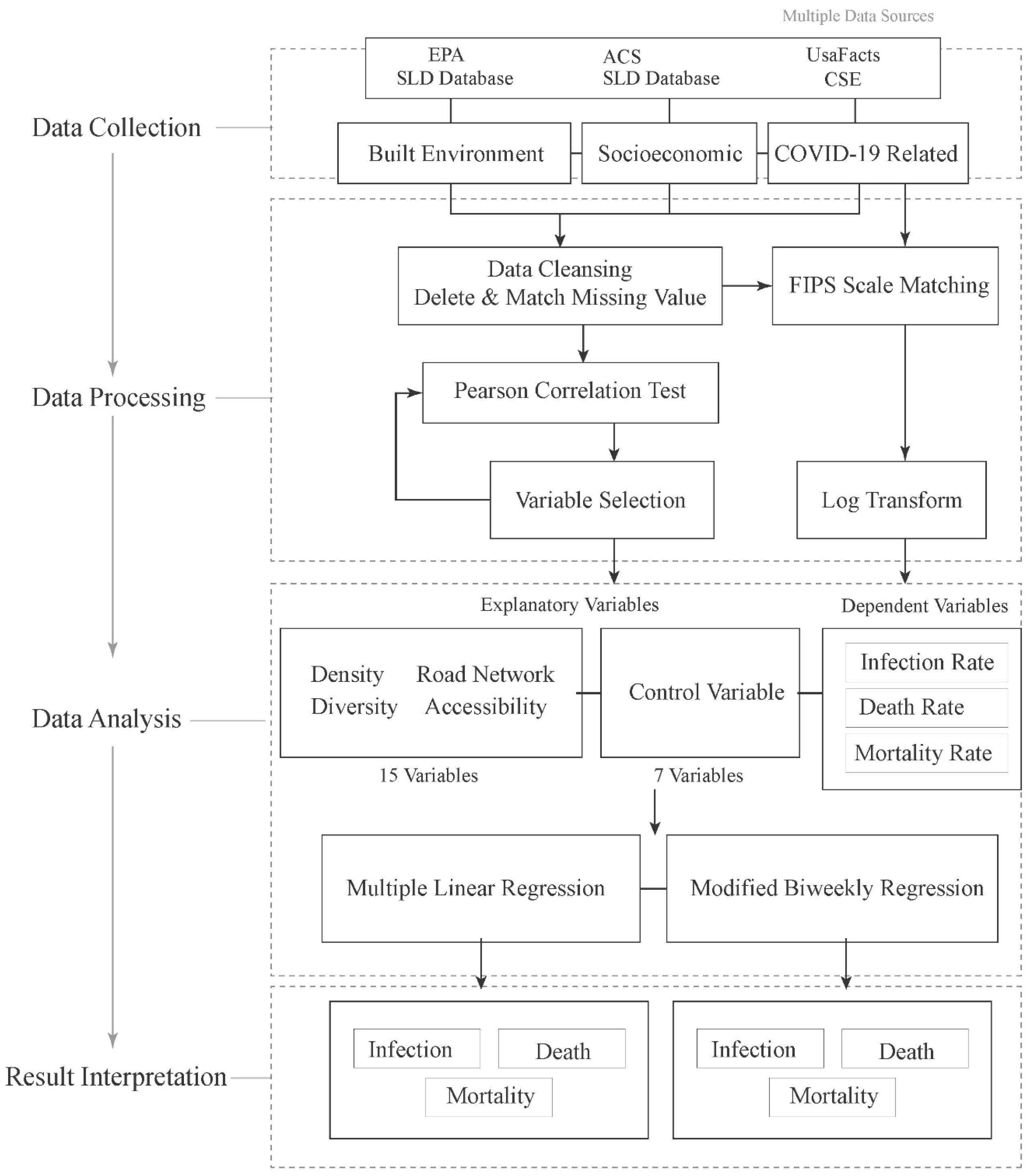
2.1. Research Framework

The overall framework of the study is displayed in Figure 1. We collected variables of the built environment, socioeconomic, and COVID-19 cases from multiple data sources. A set of data cleansing and variable processing procedures was then conducted to align the data consistency in scale and format. We conducted the Pearson Correlation Test to eliminate potential multicollinearity variables and finalized fifteen built environment variables in four categories and seven socioeconomics variables. Multiple linear regression and modified temporal linear regression models were then applied for data analysis.

2.2. Study Area and Data Collection

COVID-related data were collected from UsaFacts.org, a government data aggregation platform that directly uses information from the CDC and the state health department websites. Supplementary Materials list the websites of the state health department. The datasets include the daily confirmed COVID-19 cases and deaths of 3141 counties in the United States. Additional variables, including infection rate, death rate, and mortality rate were derived from 1 March to 8 June 2020. Calculations of the variables were referred to the procedures of coronavirus Data Repository by Johns Hopkins University Center for System and Engineering (CSE).

The built environment, socioeconomic, and demographic data were collected from the United States Environmental Protection Agency (EPA) Smart Location Database (SLD), which summarizes the characteristics of the population, the built environment, transit accessibility at the census block level across the entire United States. The original datasets contained over a hundred distinct variables that can be classified into seven categories: demographics, employment, density, diversity, design, transit, and destination accessibility. We selected a subset of variables that are the most relevant to our research questions from each of the categories. The variables EPA provided were collected from various data sources including U.S. Census, American Community Service (ACS) 2010, Census LEHD, and NAVSTREETS. Others were derived from geographic information systems using ArcGIS.

Data aggregation procedures were also implemented to merge the COVID-19, the SLD, and other datasets. Smart location data were measured at the census block level, which was smaller than the county level measurement of the coronavirus dataset. Therefore, we aggregated them to the county level. The SLD variables and the COVID-19 dataset were matched using the county Federal Information Processing Standard (FIPS) code. Table S1 in the Supplementary Materials lists the name of the selected variables and their corresponding descriptions.

2.3. Data Processing and Regression Models

2.3.1. Outcome Variables

The three outcomes are infection rate, death rate, and mortality rate (or case fatality rate). Infection rate and death rate are calculated based on the number of people who tested positive for COVID, per 100,000 population, which have been used as standard indications of disease influence in most epidemiology studies. Mortality rate is calculated by dividing the number of deaths by the number of infections, and can be over hundred percent due to the exceed amount of deaths in the current week over previous weeks.

2.3.2. Variable Processing

The original source layer was extracted from NAVTEQ Streets that includes the shape file of the infrastructure network links with the corresponding attributes such as functional class (automobile, bicycle, pedestrian), travel direction, and speed category. Then, streets were aggregated into different mode of traffic categories; intersections and traveling miles were counted utilizing boundaries of individual county, and final density measurement was calculated by dividing the miles and intersections by total land area of each county. We selected a few variables to exhibit the deriving processes:

Regional Diversity

The regional diversity variable measures the relative deviation of the average ratio of workers per jobs ratio in the census block group over the average ratio of workers per jobs in the whole core-based statistical area. The calculation of the regional diversity follows:

$$R_{div}=1-\left|\frac{b\left(W_t+T_E\right)}{b\left(W_t-T_E\right)}\right|,$$

(1)

where $R_{div}$ is the regional diversity variable; b is the ratio of population over employment of the core-based statistical area; $W_t$ is the total household workers in census block group; and $T_E$ is the total number of jobs in the census block group.

Job Equilibrium Index (JEI)

The regional diversity workers per jobs equilibrium index is calculated as follows:

$${\mathsf{{\rm I}}}_{wj}={\displaystyle \sum }_{n=0}^{\infty }\frac{1}{n!}\left(-\left|\frac{W_t}{T_E}\right|-1\right),$$

(2)

where ${\mathsf{{\rm I}}}_{wj}$ represents the equilibrium index of workers per jobs; $W_t$ represents the total number of workers in the census block group; and $T_E$ represents the total number of employments in the census block group. The closer the result index to integer one, the more balance maintained between workers and actual employment in the area.

Job Accessibility

The destination accessibility for census block group is calculated as follows:

$$A_j={\displaystyle \sum }_{k=1}^n{P}_{wj}*f{\left(d\right)}_{jk},$$

(3)

where $A_j$ is the measurement of accessibility for census block group j; $P_{wj}$ is the working-age population in census block group k; and $f{\left(d\right)}_{jk}$ is the function of impedance measurement between census block group j and k.

2.3.3. Ordinary Least Square Analysis

Three ordinary least square (OLS) regressions were implemented to examine the correlation between the dependent variables and independent variables. Dependent variables were infection rate per 100,000 population, death rate per 100,000 population, and mortality rate. Two modeling frameworks are used. One is for the entire study period and the other for biweekly period to observe temporal variation. All dependent variables are log-transformed as suggested by Sun (2020). The OLS model can be expressed as follows:

$$y_i={\beta }_1{x}_i+{\beta }_2{U}_i+{\beta }_3{P}_i+{\beta }_4{I}_i+{\beta }_5{N}_i+{\beta }_6{M}_i+{\epsilon }_i,$$

(4)

where $y_i$ represents the study outcomes, $x_i$, $U_i$, $P_i$, $I_i$, $N_i$, $M_i$, ${\epsilon }_i$, represent the i observation of the various categories of the independent variable including socioeconomics, density, diversity, road network, transit, and accessibility variables; and ${\epsilon }_i$ is the standard error.

Bi-weekly regression analysis is also implemented for an effective temporal analysis of the impact of the built environment on disease transmission. The dependent variables are segmented into 14-day periods, distinguishing the significance of the built environment variables in a biweekly manner.

3. Results

3.1. Descriptive Summary of COVID-19 and the Built Environment Variables

The spatial distribution of COVID-19 cases is shown in Figure 2 and the descriptive summary is presented in Supplementary Materials Table S2. The average number of infections per 100,000 people, from 1 March to 8 June, was 314.11, with a standard deviation of 596.85. The average death rate was 12.75%, with a standard deviation of 28.35. The average mortality rate was 3.3%, with a standard deviation of 5.21. In terms of the biweekly measures, a steadily increasing trend was observed for the average infection rate from the beginning of March to the end of April. The infection rate peaked at the fifth bi-week, with an average of 77.44 infections per 100,000 population. The maximum number of infection rates also displayed a similar trend, with a peak of 11,653.67 infections in the fifth bi-week. In terms of the death rate, the increasing trend only began after the third bi-week. The maximum number of deaths peaked at the sixth bi-week, with 212.84 deaths per 100,000 population. In terms of the mortality rate, a general increasing trend was observed from the first bi-week to the fifth bi-week. The average mortality rate peaked in the sixth bi-week with a value of 3.99%, and then started to decrease to 3.4% by the end of the seventh bi-week. The maximum mortality rate stayed relatively stable around 100%, indicating counties maintained the same amount of death numbers as the infected numbers.

The spatial distribution is shown in Figure 3 and the statistical summary of the built environment variables is shown in

Table 1. Summary of the built environment variables.

Variable	Mean	Std. Dev.	Min	Max
Socioeconomic
Population	104.59	333.65	0.27	10,039.11
Senior population	0.20	0.05	0.05	0.58
Unemployment	4.00	1.46	1.40	18.30
Population change	−0.04	0.38	−0.89	2.80
Working age population	0.77	0.04	0.58	0.98
Car ownership	0.04	0.04	0.00	0.49
Change of employment	−0.10	1.50	−39.49	1.00
Density
Residential density	4.25	8.07	0.00	112.63
Population density	9.76	18.35	0.00	291.53
Employment density	3.05	7.77	0.00	177.55
Diversity (Job and Household)
Jobs per household	1.13	1.20	0.00	28.32
Job diversity	0.17	0.09	0.00	0.99
Job equilibrium	0.29	0.11	0.00	0.99
Road network
Total road density	14.19	6.76	0.39	45.42
Auto-oriented road density	1.99	1.50	0.00	17.01
Pedestrian-oriented road density	63.63	38.10	0.10	382.02
People-oriented street intersection	1.15	1.37	0.00	24.78
Auto-oriented street intersection	10.95	9.08	0.00	140.44
Accessibility
Transit proximity	143.50	167.26	0.00	1098.57
Transit-oriented job access	0.03	0.09	0.00	1.00
Transit frequency	422.61	2468.38	0.00	118,204.78
Auto-oriented job access	112.16	138.70	0.00	1134.71
Workforce access	177.53	225.92	0.32	1345.42

. The average county population was 104.59, with a standard deviation of 333.65. The largest county by population was Los Angeles County in California (10,039,107), while the smallest county was King County in Texas (only 272). Ranked by the number of senior citizens, Los Angeles County was also the first while King County was the last. The highest percentage of senior citizens was Sumter County, Florida with nearly 58.2% of its population aged above 65, while the lowest was Chattahoochee County, Georgia, with only 4.8% senior citizens. In terms of unemployment, the highest and lowest numbers also occurred in Los Angeles County and King County. The highest and lowest rates of unemployment, however, occurred at Imperial County in California and Mountrail County in North Dakota, respectively. For the built environment variables, the highest gross density county was New York County, which comprised Manhattan as the core urban area. The second highest gross density county was Kings County in New York State, which comprises the Brooklyn area. The highest total road network density county was also New York County in New York State, followed by the Cook County that comprises the Chicago metropolitan area.

3.2. OLS Regressions on Infection Rate, Death Rate, and Mortality Rate

The results of the OLS regressions are shown in

Table 2. Results of the OLS analyses.

	(1)	(2)	(3)
	Infection	Death	Mortality
Socioeconomic
Population	−0.0000 **	−0.0000 **	−0.0000 ***
Senior population	−1.1600 ***	0.0928	0.3985
Unemployment	−0.0164 **	0.0062	0.0223 ***
Population change	−0.0475 *	0.0604 *	0.0247
Working age population	−2.3170 ***	−3.1452 ***	−0.0098
Car ownership	0.9962 ***	1.8808 ***	0.5162 **
Change of employment	0.0115	0.0202 ***	0.0064
Density
Residential density	0.0676 *	0.0515	0.0631 **
Population density	−0.0472 ***	−0.0578 ***	−0.0514 ***
Employment density	−0.0102	0.0175	0.0146
Diversity (Job and Household)
Jobs per household	0.0879 **	0.0197	−0.0586 **
Job diversity	0.2972 **	−0.2673 *	0.3513 ***
Job equilibrium	−0.1647	−0.6630 ***	−0.2035 ***
Road network
Total road density	0.1714 ***	0.0704 **	0.1302 ***
Auto-oriented road density	−0.1860 ***	0.0992	0.0033
Pedestrian-oriented road density	−0.1329 ***	0.0197	−0.0804 ***
People-oriented street intersection	−0.0086 ***	−0.0088 ***	−0.0071 ***
Auto-oriented street intersection	−0.0167	−0.0783	−0.0781 **
Accessibility
Transit proximity	0.0000	−0.0008 ***	0.0001
Transit-oriented job access	0.7617	0.6724	0.0087
Transit frequency	0.0000	0.0000	0.0000
Auto-oriented job access	−0.0000	−0.0000 **	−0.0000 ***
Population access	0.0000 ***	0.0000 ***	0.0000 ***

Note: Levels of significance were recorded at *** p < 0.001, ** p < 0.01, * p < 0.05.

. The three log-transformed dependent variables were the total infection rate, total death rate, and total mortality rate. For the infection rate model, nine built environment variables were statistically significantly correlated to the infection rate. Residential density was positively correlated to the infection rate: every 0.068 housing units per acre increase led to one log point of increase in the infection rate. However, the population density was negatively correlated to infection rate: every 0.047 people per acre decrease led to one log point of increase in the infection rate. Among the diversity indicators, jobs per household was positively associated with the infection rate, meaning the more working people in the household, the higher chance other family member will be infected. In the road network category, auto-oriented road density exhibited a positive association, while the auto-oriented street intersection was the opposite. Every 0.171 miles per acre increase in auto-oriented road density was associated with one unit (log point) increase in infection rate; every 0.009 intersections per acre decrease in pedestrian-oriented road density was associated with one unit increase in infection rate. Every 0.82 percent decrease in the employment transit proportion was associated with a one-unit increase in infection rate. In the accessibility category, population accessibility had positive correlations with the infection rate.

For the death rate model, eight built environment variables showed a significant correlation with the dependent variables. The total road density was positively correlated with death rate, while street intersection density maintained negative correlations with death rate. Every seven percent increase in total road density led to one log point of increase in death rate. On the other hand, the pedestrian-oriented street intersection density was negatively correlated to death rate, meaning that counties with higher pedestrian intersections correlated to a lower death rate. The population density was also negatively correlated to the death rate: every 0.058 people per acre decrease in population density results in a one log point increase in death rate. This might be caused by the condition where the lower population density area lacked sufficient medical resources compared to the higher population density area. In the diversity category, a negative association exists between the jobs equilibrium and death rate. The lowering of the equilibrium index means that workforce supply does not match local job demands, and the number of workers is lower than the number of jobs. In other words, counties with an insufficient workforce were facing a higher risk of death from COVID-19. For the socioeconomic variables, the unemployment rate maintained a positive correlation to the death rate. The percentage change of population and employment between 2010 and 2019 both revealed negative relationships.

For the mortality rate model, eleven built environment variables showed a significant correlation with the dependent variable. The population density was negatively correlated to the mortality rate, meaning every 0.05 people per acre decrease in population density led to one log point increase in mortality rate. On the other side, residential density variables displayed a positive coefficient, meaning that the higher the residential density, the higher the risks of death when infected. For the diversity category, we found a positive association between job diversity and mortality rate, with a coefficient of 0.35, meaning that the higher the ratio between employments and population in a county, the higher the risks of mortality. The total road density was positively correlated to the mortality rate; pedestrian road density received a negative coefficient, meaning that counties with more pedestrian road areas generally had lower risks of fatality when infected. Every 0.13 miles per acre increase in total road density led to one log point of increase in mortality rate. The unemployment rate had a positive correlation with the mortality rate: every one percent increase in the unemployment rate led to a 0.022 unit increase in mortality rate.

In addition to the built environment variables, few socioeconomic variables were associated with the dependent variables. The senior population rate exhibited a negative correlation to the infection rate, indicating every one percent increase in the senior population yielded a drop of 1.16 units of logged infection rate. A negative association was also found between the unemployment rate and the infection rate. Additionally, population changes, car ownership, and working age population were all significantly associated with the infection rate.

3.3. Biweekly Analysis

Table 3. Biweekly infection rate regression.

	(1)	(2)	(3)	(4)	(5)	(6)	(7)
Variables	Weeks 1–2	Weeks 3–4	Weeks 5–6	Weeks 7–8	Weeks 9–10	Weeks 11–12	Weeks 13–14
Socioeconomic
Population	−0.0000 ***	0.0000 **	0.0000	0.0000	−0.0000	−0.0000	0.0000
Senior population	−0.2977	−1.1371 ***	−2.1156 ***	−2.3441 ***	−2.2181 ***	−1.8857 ***	−1.4291 ***
Unemployment	0.0410 ***	−0.0153 *	0.0217 **	0.0095	−0.0066	−0.0024	0.0019
Population change	0.0107	0.0623 *	0.1015 ***	0.0460	−0.0288	−0.0110	0.0782 **
Working age population	2.3823 ***	−0.7323	1.2620 **	−0.3882	−2.1036 ***	−3.2293 ***	−4.3355 ***
Car ownership	−0.7978 ***	0.5767 *	1.3240 ***	1.4903 ***	1.0235 **	1.8022 ***	1.5565 ***
Change of employment	0.0000	−0.0000 **	−0.0000	−0.0000	−0.0000	−0.0000	−0.0000
Density
Residential density	−0.1784 ***	0.2420 ***	0.0883 *	0.0503	0.0405	0.0468	0.0580
Population density	0.0563 ***	−0.1284 ***	−0.0860 ***	−0.0714 ***	−0.0567 **	−0.0590 **	−0.0585 **
Employment density	0.0735 ***	−0.0303	0.0346	0.0423 *	0.0246	0.0213	0.0138
Diversity (Job and Household)
Jobs per household	0.1516 ***	−0.0002	−0.0157	−0.0142	0.0210	0.0939	0.1427 **
Job diversity	−0.2168 **	0.8060 ***	1.0501 ***	0.8125 ***	0.5634 ***	0.5193 ***	0.3842 **
Job equilibrium	−0.1053	−0.2133 *	−0.7651 ***	−0.8249 ***	−0.6743 ***	−0.8359 ***	−0.8070 ***
Road network
Total road density	0.0852 ***	0.1452 ***	0.3036 ***	0.3519 ***	0.3395 ***	0.3321 ***	0.2840 ***
Auto-oriented road density	−0.0342	−0.2465 ***	−0.1996 ***	−0.2119 ***	−0.0974	−0.0535	−0.1418 *
Pedestrian-oriented road density	−0.0951 ***	−0.0430	−0.1945 ***	−0.2384 ***	−0.2500 ***	−0.2355 ***	−0.1498 ***
People-oriented street intersection	0.0010	−0.0168 ***	−0.0177 ***	−0.0187 ***	−0.0154 ***	−0.0169 ***	−0.0216 ***
Auto-oriented street intersection	−0.0841 **	0.0555	−0.1447 **	−0.1534 **	−0.1991 ***	−0.2212 ***	−0.1003
Accessibility
Transit proximity	0.0003 **	0.0003	0.0002	0.0000	0.0000	−0.0001	−0.0002
Transit-oriented job access	1.8384 ***	0.9669	0.7883	0.9536	0.8895	0.6939	0.4814
Transit frequency	−0.0001 **	0.0001	0.0000	0.0000	0.0000	0.0000	0.0000
Auto-oriented job access	−0.0000	−0.0000 ***	−0.0000 ***	−0.0000 ***	−0.0000	−0.0000	−0.0000 *
Population access	0.0000	0.0000 ***	0.0000 ***	0.0000 ***	0.0000 ***	0.0000 **	0.0000 **

Note: Levels of significance were recorded at *** p < 0.001, ** p < 0.01, * p < 0.05.

,

Table 4. Biweekly logged death rate regression.

	(1)	(2)	(3)	(4)	(5)	(6)	(7)
Variables	Weeks 1–2	Weeks 3–4	Weeks 5–6	Weeks 7–8	Weeks 9–10	Weeks 11–12	Weeks 13–14
Socioeconomic
Population	0.0000 **	−0.0000 ***	−0.0000	−0.0000	−0.0000	−0.0000	−0.0000
Senior population	0.0178	−0.1554	−0.0660	−0.1180	−0.2427	0.0988	0.0239
Unemployment	0.0063 ***	0.0042	0.0126 **	0.0124 **	0.0147 **	0.0258 ***	0.0266 ***
Population change	0.0027	−0.0216 **	−0.0400 **	−0.0606 ***	−0.0549 **	−0.0717 ***	−0.0634 ***
Working age population	0.2378 ***	0.1236	−0.1212	−0.0415	−0.5071	−0.8897 **	−0.7289 **
Car ownership	−0.0911 **	0.1170	0.6333 ***	1.4228 ***	0.9599 ***	0.8446 ***	0.8679 ***
Change of employment	−0.0000 ***	0.0000 ***	−0.0000	−0.0000	−0.0000	−0.0000	0.0000
Density
Residential density	−0.0161 **	0.0137	0.0551 **	0.0240	0.0524	0.0572 *	0.0550 *
Population density	0.0106 ***	−0.0053	−0.0498 ***	−0.0505 ***	−0.0543 ***	−0.0449 ***	−0.0397 ***
Employment density	0.0019	0.0059	0.0132	0.0285 **	0.0119	−0.0050	−0.0059
Diversity (Job and Household)
Jobs per household	0.0204 ***	0.0152	0.0022	−0.0172	0.0361	0.0566 *	0.0287
Job diversity	−0.0249	0.0519	0.2367 ***	0.2673 ***	0.2065 **	0.3063 ***	0.2911 ***
Job equilibrium	−0.0280 *	−0.0064	−0.0279	−0.0961	−0.1165	−0.1839 **	−0.1669 **
Road network
Total road density	0.0253 ***	−0.0107	0.0841 ***	0.1378 ***	0.1726 ***	0.1411 ***	0.1077 ***
Auto-oriented road density	−0.0088	−0.0210	−0.1475 ***	−0.1686 ***	−0.2446 ***	−0.1508 ***	−0.1128 **
Pedestrian-oriented road density	−0.0226 ***	−0.0012	−0.0560 ***	−0.0865 ***	−0.1381 ***	−0.1175 ***	−0.0884 ***
People-oriented street intersection	−0.0005	0.0008	−0.0045 ***	−0.0079 ***	−0.0063 ***	−0.0047 ***	−0.0037 **
Auto-oriented street intersection	−0.0212 ***	0.0162	0.0096	−0.0110	−0.0073	−0.0324	−0.0450
Accessibility
Transit proximity	0.0000	−0.0004 ***	0.0001	0.0002	0.0004 ***	0.0003 **	0.0001
Transit-oriented job access	−0.4898 ***	0.7034 ***	1.1896 ***	1.0467 **	1.1786 ***	0.6838	0.2316
Transit frequency	0.0000	−0.0000 **	−0.0000	−0.0000	−0.0000	−0.0000	0.0000
Auto-oriented job access	0.0000 ***	−0.0000 ***	−0.0000 ***	−0.0000 ***	−0.0000 *	−0.0000	−0.0000
Population access	−0.0000 ***	0.0000 ***	0.0000 ***	0.0000 ***	0.0000 ***	0.0000 **	0.0000 **

Note: Levels of significance were recorded at *** p < 0.001, ** p < 0.01, * p < 0.05.

and

Table 5. Biweekly logged mortality rate regression.

	(1)	(2)	(3)	(4)	(5)	(6)	(7)
Variables	Weeks 1–2	Weeks 3–4	Weeks 5–6	Weeks 7–8	Weeks 9–10	Weeks 11–12	Weeks 13–14
Socioeconomic
Population	0.0000	−0.0000	−0.0000	0.0000	0.0000	−0.0000	−0.0000
Senior population	0.0310	−0.1608	0.1861	−0.1007	0.0204	0.2735	−0.0408
Unemployment	0.0001	0.0081 **	0.0109 **	0.0051	0.0104 *	0.0142 **	0.0128 **
Population change	0.0059	0.0384 ***	0.0273	0.0230	0.0394 *	0.0064	−0.0282
Working age population	−0.0394	0.2268	−0.4536	0.1763	−0.1947	−0.2548	0.0734
Car ownership	0.0163	−0.0435	0.2063	0.9745 ***	0.5998 ***	0.6388 ***	0.5889 ***
Change of employment	−0.0000	0.0000	0.0000	−0.0000	−0.0000	−0.0000	0.0000
Density
Residential density	0.0058	0.0021	0.0584 *	0.0462	0.1240 ***	0.0839 **	0.0911 ***
Population density	−0.0070 **	0.0000	−0.0354 ***	−0.0469 ***	−0.0795 ***	−0.0620 ***	−0.0602 ***
Employment density	0.0024	0.0028	0.0024	0.0229	0.0055	0.0115	0.0054
Diversity (Job and Household)
Jobs per household	−0.0086	0.0080	−0.0270	−0.0679 **	−0.0181	−0.0297	−0.0533 *
Job diversity	0.0312	0.0632	0.4663 ***	0.4220 ***	0.2311 **	0.4148 ***	0.4114 ***
Job equilibrium	0.0185	−0.0416	−0.1295 *	−0.1690 **	−0.1008	−0.1882 **	−0.2035 ***
Road network	−0.0086	0.0080	−0.0270	−0.0679 **	−0.0181	−0.0297	−0.0533 *
Total road density	−0.0054	0.0562 ***	0.1003 ***	0.1413 ***	0.1880 ***	0.1568 ***	0.1543 ***
Auto-oriented road density	0.0120	−0.0114	−0.0481	−0.0097	−0.1305 ***	−0.0677	−0.1238 ***
Pedestrian-oriented road density	0.0084	−0.0415 ***	−0.0488 **	−0.0633 **	−0.1214 ***	−0.1173 ***	−0.1252 ***
People-oriented street intersection	−0.0001	−0.0025 **	−0.0075 ***	−0.0109 ***	−0.0103 ***	−0.0060 ***	−0.0046 ***
Auto-oriented street intersection	0.0055	−0.0306	−0.0051	−0.0627	−0.0531	−0.0817 **	−0.0796 **
Accessibility
Transit proximity	0.0001 ***	−0.0000	0.0000	0.0001	0.0002	0.0002 *	0.0002 *
Transit-oriented job access	0.3504 ***	−0.5247 *	−0.4465	−0.3110	−0.2484	−0.0307	−0.2504
Transit frequency	−0.0000	−0.0000	0.0000	−0.0000	0.0000	−0.0000	0.0000
Auto-oriented job access	−0.0000	−0.0000 *	−0.0000 ***	−0.0000 ***	−0.0000 ***	−0.0000 ***	−0.0000 ***
Population access	0.0000	0.0000 *	0.0000 ***	0.0000 ***	0.0000 ***	0.0000 ***	0.0000 ***

Note: Levels of significance were recorded at *** p < 0.001, ** p < 0.01, * p < 0.05.

display the biweekly models’ results utilizing infection rate, death rate, and mortality rate, respectively. Figure 4 and Figure S1 also display the results with selected significant built environment attributes. We observed a strong, positive, and significant association between the total road density and the spread of the virus, as shown in Table 3. The coefficient increased from 0.08 at the first week to 0.34 during weeks 7–8, and remain positive above 0.02 for the rest of the period. On the other hand, auto-oriented density received a negative coefficient of 0.018 since weeks 5–6. The different signs of the coefficients indicated a heavier weight of the positive effect of pedestrian road density, resulting in a positive sign in the total road density. In the density category, population density yielded a positive correlation in weeks 1–2, but the coefficient became negative and decreased over time. On the other hand, residential density was positively correlated to the spread of the virus from weeks 1–4, and the significance disappeared afterward. It is also worth mentioning that there was a positive association between transit proximity and infection rate. Significance also dissipated after the fourth week. In addition, the transit-oriented job accessibility also yielded a positive correlation with the infection rate in weeks 1–2, and the significance dissipated after the second week.

The biweekly death rate model is shown in Table 4. Similar to the biweekly infection model, the total road density again maintained a positive correlation to the death rate over time. The total road density coefficient increased from 0.025 on weeks 1 and 2 to 0.173 on weeks 7 and 8. The auto-oriented road density and pedestrian-oriented road density were both negatively correlated to the death rate from weeks 5–6, meaning that the lower the pedestrian road density, the higher the chances of death. In the first two weeks, only the pedestrian-oriented road density was negatively correlated to the death rate, while no significant correlation existed between the auto-oriented road density and the death rate. Transit-oriented job accessibility yielded a significant, negative correlation to the death rate in weeks 1–2, with a coefficient of −0.49, and became positively correlated to the death rate starting from weeks 3–4, with a coefficient reaching as high as 1.19 in weeks 9–10. In the density category, population density yielded a positive correlation in weeks 1–2 with a coefficient of 0.011, but became negative from weeks 5–14. On the other hand, the residential density, yielded a negative correlation to the death rate in weeks 1–2, and became positive during weeks 5–6 and 11–14. In the diversity category, jobs per household was positively correlated to the death rate on weeks 1–2, with a coefficient of 0.02, and no significance was found afterward.

The results of the biweekly mortality model, as shown in Table 5, revealed that the total road network density was positively correlated to the mortality rate from weeks 3–14. The coefficient had an increasing trend peaked at 0.188 in weeks 9–10. The pedestrian road density was negatively correlated to the mortality rate from week 3–14, with a decreasing trend ranging from 0.041 to 0.121. In the density category, the population density was negatively correlated to the mortality rate in weeks 1–2 and 5–14, with coefficients ranging from 0.007 to 0.079. The residential density, on the other hand, maintained a positive correlation to the mortality rate in weeks 5–6 and 9–14, with coefficients ranging from 0.058 to 0.124.

4. Discussion

The current study explored how the built environment contributed to the COVID-19 pandemic in the United States. The study verifies the hypothesis that key built environment features are correlated to the COVID infection rate, death rate, and mortality rate differentially, respectively. Notably, among all the built environment attributes, road network, street intersection, population density, and residential density all play a significant role in affecting the pandemic prevalence. The study reveals underlying susceptibility based on regional built environment characteristics and effectively demonstrates the significance of evaluating built environment in addition to regional socioeconomic background on the prevalence of the COVID-19 pandemic.

In terms of the relationships between the built environment and infection rate, death rate, and mortality rate, we found a negative correlation between population density and prevalence of COVID-19, which was counterintuitive to the common understanding that the denser the population, the more infectious the virus (Hamidi, 2020b). Different from the existing study analyzing density and virus transmission, our study showed that the temporal regression, on the other hand, indicated a positive correlation between population density and prevalence of the virus in the first two weeks and the sign of significance became negative afterward. It suggested that high population density areas, such as urban areas, were more infectious during the first two weeks; low population density areas, such as suburbs and rural areas, became more infectious since the third week. Such a phenomenon might be explained by the potential different disease control measures implemented in an urban and rural context: trivial attention was put on disease prevention from the low-density area population, while populations in the high-density area maintained a relatively more prudent attitude toward COVID-19, which led to more preventive behaviors from the individual. Further investigation is needed for verification. Moreover, residential density displayed reverse results that were the opposite of population density, in which a negative correlation appeared in the initial two weeks and became negative in later two weeks. There was also no significant correlation found between employment density and virus prevalence. Aligning with the perspective of population density, all of these indicators displayed that a relatively high residential density area, with low population density and away from the concentration of employment, became more vulnerable to pandemic infection starting from week 3, which was the period where the federal government announced the national lockdown. The policy implication is that reducing population density can only prevent the spread of the virus in the initial two weeks; afterward, more attention should be paid to the low-density population areas. Key pandemic prevention measures should also be implemented in the high residential areas in the initial four weeks by local authorities. After all, even under the condition of national lockdowns, people in residential areas might lose attention to the control policies and expose themselves to high chances of infection.

The study also found a consistent positive correlation between the total road network density and the prevalence of COVID-19 for all study periods, which verified our hypothesis that the commutable disease is more infectious in high road density areas. It also verified the argument proposed in Hamidi et al. (2020a) that connectivity was an essential factor for virus transmission. On the other hand, both the pedestrian-oriented road density and people-oriented street intersection density were negatively correlated to the infection rate, indicating that counties with lower street intersection and pedestrian sidewalk, generally in a suburb or rural area, received higher chances of infection, which supplemented the argument that high infection rate in low population area with a downward decreasing coefficient trend. This again stresses the significance of awareness of disease prevention should be stressed in places with low population density, such as the suburbs and rural areas.

Transit accessibility played an essential role in virus transmission during the first four weeks of the pandemic. The accessibility of transit-oriented jobs was highly correlated to the infection rate in the first two weeks, indicating that a higher proportion of employment within 0.25 miles of transit facility was subjected to a higher chance of infection. This could be supplemented by the positive association of employment density and infection rate, which were also highly correlated in the first two weeks only and then became non-significant afterward. On the other hand, though its significance was trivial, the negative coefficient of transit frequency in the first two weeks indicated that counties with lower transit frequency per square mile were subjected to higher infection rates. This may be linked to the fact that low transit frequency is often associated with rural or suburbs where low population density receives greater infection chances as mentioned above. This indicated that policymakers should advocate different public transit accessibility to different groups of population in different areas, which correspond to a similar argument proposed in Palm et al. (2021) [32].

All significant variables for the total infection, death, and mortality rate models are displayed in Supplementary Materials Table S3. In this study, we also tested several socioeconomic variables as control variables. Previous empirical study suggested that high risks existed among the senior population during the early stage of the pandemic (Sun et al., 2020). However, we did not discover a significant correlation between senior population rate and COVID-19 death rate in our study. This could be explained by the lack of detailed data on the socioeconomic status of individual deaths. On the other hand, we observed a consistent positive correlation between the unemployment rate and death rate across the entire study period. The coefficient was statically significant and maintained an increasing trend, which indicated that counties suffered from a high unemployment rate, in general, also suffered from lack of medical resources needed to mitigate the fatality of the pandemic, and further incorporation of medical capacity data may verify the statement.

Overall, the research demonstrates the significance of evaluating the effect of the built environment on the transmission of coronavirus pandemics. The study suggests that public health authorities should also take into account the effect of built structure when distributing medical resources across different regions of the states. The limitation of the study includes the lack of investigation of causal relationship between the dependent and explanatory variables as the current empirical results only suggest correlational relationship. In addition, as the vaccination programs have been deployed progressively, it is necessary to consider the spatiality of such deployment that the current study neglects to consider. Future studies should further investigate the causal relationship between these variables with the incorporation of vaccination effect and spatial autocorrelation. Additional models should include geographically weighted regression, spatial lag, and spatial error models, to emphasize the local effect of the vaccination as an embedded attribute of the build environment impact. Additionally, the built environment attributes should also be considered to address various climate and geographical conditions. In addition, spatial distribution and quality of health facilities should also be included to reflect treatment capacities.

5. Conclusions

This study investigated the relationship between the COVID-19 pandemic and the built environment of the United States. The results contributed to the field by recognizing research gaps between the spatial distribution of COVID-19 and the built environment attributes at the county level. A consistent result of this study indicated the significant role of the built environment on the spread of COVID-19. When allocating resources, policymaker should not only consider the vulnerability of the population group and their corresponding socioeconomic status, but also take into consideration the effect of the built environment as an active transmission channel and plan countermeasures against the spread of viruses beforehand. The biweekly models indicated a strong temporal variation of the impact of the built environment on the prevalence of COVID-19. Although the majority of the built environment variables were static over time, the corresponding impact changed over time. Therefore, it is advantageous to actively monitor the impact and implement countermeasures swiftly and accordingly under local contexts.

Using socioeconomic, density, diversity, accessibility, and transit network variables, we investigated the impact between the built environment and pandemic infection rate, death rate, and mortality rate. The results indicated that: (1) the built environment had significant impacts on the spread of the COVID-19 at the initial stage; (2) different built environment variables reacted differently to infection rate, death rate, and mortality rate: road network density maintained the most impactful category among all; (3) population density only maintained a positive correlation to the prevalence of COVID-19 during the first two weeks, and the correlation became negative afterward; (4) a consistently positive and increasing correlation was observed between unemployment rate and death rate across the entire study period; and (5) during the first four weeks of the pandemic, transit accessibility contributed significantly to the infection rate, and the accessibility of transit-oriented jobs highly correlated to infection rate in the first two weeks.

References

1. Sun, F.; Matthews, S.A.; Yang, T.-C.; Hu, M.-H. A spatial analysis of the COVID-19 period prevalence in U.S. counties through June 28, 2020: Where geography matters? Ann. Epidemiol. 2020, 52, 54–59.e1. [Google Scholar] [CrossRef] [PubMed]
2. Hamidi, S.; Ewing, R.; Sabouri, S. Longitudinal analyses of the relationship between development density and the COVID-19 morbidity and mortality rates: Early evidence from 1165 metropolitan counties in the United States. Health Place 2020, 64, 102378. [Google Scholar] [CrossRef] [PubMed]
3. Paul, R.; Arif, A.A.; Adeyemi, O.; Ghosh, S.; Han, D. Progression of COVID-19 From Urban to Rural Areas in the United States: A Spatiotemporal Analysis of Prevalence Rates. J. Rural Health 2020, 36, 591–601. [Google Scholar] [CrossRef] [PubMed]
4. Zenic, N.; Taiar, R.; Gilic, B.; Blazevic, M.; Maric, D.; Pojskic, H.; Sekulic, D. Levels and Changes of Physical Activity in Adolescents during the COVID-19 Pandemic: Contextualizing Urban vs. Rural Living Environment. Appl. Sci. 2020, 10, 3997. [Google Scholar] [CrossRef]
5. Liu, C.; Liu, Z.; Guan, C. The impacts of the built environment on the incidence rate of COVID-19: A case study of King County, Washington. Sustain. Cities Soc. 2021, 74, 103144. [Google Scholar] [CrossRef]
6. Zulu, L.C.; Kalipeni, E.; Johannes, E. Analyzing spatial clustering and the spatiotemporal nature and trends of HIV/AIDS prevalence using GIS: The case of Malawi, 1994–2010. BMC Infect. Dis. 2014, 14, 285. [Google Scholar] [CrossRef] [Green Version]
7. Brizuela, N.G.; García-Chan, N.; Pulido, H.G.; Chowell, G. Understanding the role of urban design in disease spreading. Proc. R. Soc. A 2021, 477, 20200524. [Google Scholar] [CrossRef]
8. Xiao, H.; Lin, X.; Chowell, G.; Huang, C.; Gao, L.; Chen, B.; Wang, Z.; Zhou, L.; He, X.; Liu, H.; et al. Urban structure and the risk of influenza A (H1N1) outbreaks in municipal districts. Chin. Sci. Bull. 2014, 59, 554–562. [Google Scholar] [CrossRef]
9. Apolloni, A.; Poletto, C.; Colizza, V. Age-specific contacts and travel patterns in the spatial spread of 2009 H1N1 influenza pandemic. BMC Infect. Dis. 2013, 13, 176. [Google Scholar] [CrossRef] [Green Version]
10. Mao, L.; Bian, L. Spatial–temporal transmission of influenza and its health risks in an urbanized area. Comput. Environ. Urban Syst. 2010, 34, 204–215. [Google Scholar] [CrossRef]
11. Cai, J.; Xu, B.; Chan, K.K.Y.; Zhang, X.; Zhang, B.; Chen, Z.; Xu, B. Roles of Different Transport Modes in the Spatial Spread of the 2009 Influenza A(H1N1) Pandemic in Mainland China. Int. J. Environ. Res. Public Health 2019, 16, 222. [Google Scholar] [CrossRef] [PubMed] [Green Version]
12. Maliszewski, P.J.; Wei, R. Ecological factors associated with pandemic influenza A (H1N1) hospitalization rates in California, USA: A geospatial analysis. Geospat. Health 2011, 6, 95. [Google Scholar] [CrossRef] [PubMed] [Green Version]
13. Dalziel, B.D.; Kissler, S.; Gog, J.R.; Viboud, C.; Bjørnstad, O.N.; Metcalf, C.J.E.; Grenfell, B.T. Urbanization and humidity shape the intensity of influenza epidemics in U.S. cities. Science 2018, 362, 75–79. [Google Scholar] [CrossRef] [PubMed] [Green Version]
14. Dowd, J.B.; Andriano, L.; Brazel, D.M.; Rotondi, V.; Block, P.; Ding, X.; Liu, Y.; Mills, M.C. Demographic science aids in understanding the spread and fatality rates of COVID-19. Proc. Natl. Acad. Sci. USA 2020, 117, 9696–9698. [Google Scholar] [CrossRef] [Green Version]
15. Lee, B.; Raszka, W.V. COVID-19 Transmission and Children: The Child Is Not to Blame. Pediatrics 2020, 146, e2020004879. [Google Scholar] [CrossRef]
16. Millett, G.A.; Jones, A.T.; Benkeser, D.; Baral, S.; Mercer, L.; Beyrer, C.; Honermann, B.; Lankiewicz, E.; Mena, L.; Crowley, J.S.; et al. Assessing differential impacts of COVID-19 on black communities. Ann. Epidemiol. 2020, 47, 37–44. [Google Scholar] [CrossRef]
17. Yancy, C.W. COVID-19 and African Americans. JAMA J. Am. Med Assoc. 2020, 323, 1891. [Google Scholar] [CrossRef] [Green Version]
18. Cordes, J.; Castro, M.C. Spatial analysis of COVID-19 clusters and contextual factors in New York City. Spat. Spatio-Temporal Epidemiol. 2020, 34, 100355. [Google Scholar] [CrossRef]
19. Sannigrahi, S.; Pilla, F.; Basu, B.; Basu, A.S. The overall mortality caused by COVID-19 in the European region is highly associated with demographic composition: A spatial regression-based approach. arXiv 2020, arXiv:2005.04029. [Google Scholar]
20. Desai, N.; Neyaz, A.; Szabolcs, A.; Shih, A.R.; Chen, J.H.; Thapar, V.; Nieman, L.T.; Solovyov, A.; Mehta, A.; Lieb, D.J.; et al. Temporal and spatial heterogeneity of host response to SARS-CoV-2 pulmonary infection. Nat. Commun. 2020, 11, 1–15. [Google Scholar] [CrossRef]
21. Hamidi, S.; Sabouri, S.; Ewing, R. Does Density Aggravate the COVID-19 Pandemic? Early Findings and Lessons for Planners. J. Am. Plan. Assoc. 2020, 86, 495–509. [Google Scholar] [CrossRef]
22. Zhang, C.H.; Schwartz, G.G. Spatial Disparities in Coronavirus Incidence and Mortality in the United States: An Ecological Analysis as of May 2020. J. Rural Health 2020, 36, 433–445. [Google Scholar] [CrossRef] [PubMed]
23. Skórka, P.; Grzywacz, B.; Moroń, D.; Lenda, M. The macroecology of the COVID-19 pandemic in the Anthropocene. PLoS ONE 2020, 15, e0236856. [Google Scholar] [CrossRef] [PubMed]
24. Zhang, Y.; Zhang, A.; Wang, J. Exploring the roles of high-speed train, air and coach services in the spread of COVID-19 in China. Transp. Policy 2020, 94, 24–42. [Google Scholar] [CrossRef] [PubMed]
25. Peters, D.J. Community Susceptibility and Resiliency to COVID-19 Across the Rural-Urban Continuum in the United States. J. Rural Health 2020, 36, 446–456. [Google Scholar] [CrossRef]
26. Block, P.; Hoffman, M.; Raabe, I.J.; Dowd, J.B.; Rahal, C.; Kashyap, R.; Mills, M.C. Social network-based distancing strategies to flatten the COVID-19 curve in a post-lockdown world. Nat. Hum. Behav. 2020, 4, 588–596. [Google Scholar] [CrossRef]
27. Kraemer, M.U.G.; Yang, C.-H.; Gutierrez, B.; Wu, C.-H.; Klein, B.; Pigott, D.M.; Open COVID-19 Data Working Group; du Plessis, L.; Faria, N.R.; Li, R.; et al. The effect of human mobility and control measures on the COVID-19 epidemic in China. Science 2020, 368, 493–497. [Google Scholar] [CrossRef] [Green Version]
28. Lau, M.S.Y.; Grenfell, B.; Thomas, M.; Bryan, M.; Nelson, K.; Lopman, B. Characterizing superspreading events and age-specific infectiousness of SARS-CoV-2 transmission in Georgia, USA. Proc. Natl. Acad. Sci. USA 2020, 117, 22430–22435. [Google Scholar] [CrossRef]
29. Li, B.; Peng, Y.; He, H.; Wang, M.; Feng, T. Built environment and early infection of COVID-19 in urban districts: A case study of Huangzhou. Sustain. Cities Soc. 2021, 66, 102685. [Google Scholar] [CrossRef]
30. Li, S.; Ma, S.; Zhang, J. Association of built environment attributes with the spread of COVID-19 at its initial stage in China. Sustain. Cities Soc. 2021, 67, 102752. [Google Scholar] [CrossRef]
31. Megahed, N.A.; Ghoneim, E.M. Antivirus-built environment: Lessons learned from Covid-19 pandemic. Sustain. Cities Soc. 2020, 61, 102350. [Google Scholar] [CrossRef] [PubMed]
32. Palm, M.; Allen, J.; Liu, B.; Zhang, Y.; Widener, M.; Farber, S. Riders Who Avoided Public Transit During COVID-19. J. Am. Plan. Assoc. 2021, 87, 455–469. [Google Scholar] [CrossRef]
Figure 1. Framework of the research design.
Sustainability 14 03417 g001
Figure 2. The infection, death and mortality rate of COVID-19 at the county level, 1 March to 8 June 2020. From top to bottom, the three maps represent (a) infection; (b) death; and (c) mortality rate, respectively.
Sustainability 14 03417 g002
Figure 3. The built environment variables. From top to bottom, the three maps represent: (a) residential density; (b) road network density; and (c) job accessibility, respectively. The study area includes the continental USA, Alaska, and Hawaii.
Sustainability 14 03417 g003
Figure 4. Biweekly multiple linear regressions with selected built environment attributes.
Sustainability 14 03417 g004