Abstract
This paper studies the firm-level impact of the river chief system (RCS), which is a decentralized policy in China for water protection, by investigating polluting firms’ emission abatement and the net operating profits. We have four main findings. First, on average, the RCS significantly reduced firm-level COD emissions by 3.7 percent, which was mainly caused by the emission abatement of firms in heavily polluting industries, non-state-owned firms, and firms in the eastern provinces. On the other hand, the RCS also significantly increased polluting firms’ profit by 3.1 percent, which was mainly caused by heavily polluting firms. Second, different regions adopted different strategies for pollution abatement, exhibiting a pattern consistent with the “pollution paradise” assumption in the central and western provinces. Third, polluting firms at provincial boundaries did not reduce their COD emissions, while polluting firms in the interior significantly reduced their emissions by 5.6 percent, indicating the strong free-riding incentive of local governments. Fourth, the increase in the profits of heavily polluting industries was mainly caused by the significant increase in market concentration and a possible transfer of the negative shock from the RCS along the production line. All results were also robust for firm-level NH-N emissions. This paper provides new and insightful implications for policymaking for environmental protection.
JEL Classification:
L60; Q52; Q53; Q58
1. Introduction
The rapid economic development of China since 1978 has caused severe environmental problems. In 2003, the central government officially claimed its target to be balancing the economic development and environmental sustainability. In order to align local governments’ incentives with those of the central government, stringent requirements on COD emissions and water quality improvement were built into local governors’ performance evaluations. However, the highly decentralized political regime, the information asymmetry between local governments and the central government, and the fact that economic development is still a critical measure in local leaders’ performance evaluation mitigate local governments’ efforts to reduce water pollution [1].
In 2007, the outbreak of blue algae in Tai Lake of Wuxi in Jiangsu Province caught the national attention. (Tai Lake is the third largest lake in China and is located in the south of the Jiangsu province and the north of the Zhejiang province). In the same year, Wuxi pioneered an innovative system, known as the river chief system (RCS). This system assigns leading officials of local governments to be “heads” of certain parts of rivers and lakes to enhance their incentives and responsibility for emission abatement. The responsible official’s name and contact information are carved on an iron plate planted by the part of the river or lake for which they are responsible (https://www.sohu.com/a/258892626_684405 (accessed on 15 Februray 2022)). This policy effectively improved the water quality in the Tai Lake and was later adopted by many prefectures in the Yangtz River Delta and by prefectures in several other provinces of China. In 2016, the central government officially required the RCS to be implemented in all prefectures by the end of 2018.
The RCS is generally believed to an effective strategy for reducing water pollution [2,3]. However, unlike other policies for water protection implemented by the central government with precise emission abatement targets, the RCS, as a decentralized policy, gave more freedom to local governments. Hence, there may exist heterogeneity in regulation across prefectures and industries, leading to different impacts on polluting firms. The current literature on the RCS does not investigate the firm-level impact or the heterogeneity across firms in different industries and regions. What types of firms contribute more to emission abatement? Does there exist a heterogenous impact across industries and prefectures? What are the policy implications? We aim to answer these questions by using a generalized difference-in-difference (DID) model with the propensity score matching (PSM) method to investigate the RCS’s firm-level impact on polluting manufacturing firms’ COD emission abatement and net operating profits from 2007 to 2013. Our results can deepen the understanding of the execution of the RCS and, thereby, provide rich policy implications.
We have four main findings. First, on average, the RCS significantly reduced firm-level COD emissions by 3.7%. This effect was mainly caused by the emission abatement of firms in heavily polluting industries, non-state-owned firms, and firms in the eastern provinces. On the other hand, the RCS also significantly increased polluting firms’ profit by 3.1% on average, which was mainly caused by heavily polluting firms. Second, different regions adopted different strategies for pollution abatement: Heavily polluting industries contributed significantly in terms of emission abatement in the eastern provinces, and moderately polluting industries contributed the most in the northeastern provinces. However, heavily polluting and moderately polluting firms in the central provinces and moderately polluting firms in the western provinces increased their COD emissions, which was consistent with the “pollution paradise” assumption [4,5]. Third, the increase in the profits of heavily polluting industries was mainly caused by the significant increase in market concentration. While the market concentration also increased in moderately and lightly polluting industries, their profits were not affected, indicating a possible transfer of the negative shock from the RCS along the production line. Finally, we replaced the COD emissions with ammonia nitrogen emissions (NH-N) and the net operating profit with the net total profit of polluting firms. The results were qualitatively the same, supporting the robustness of our main results.
This paper contributes to two strands of literature. The first strand is still growing, and it studies the effects of the RCS on emission abatement and policy implications. Some studies used prefectural data and found that the RCS had a significant effect on emission abatement [6]. Some concluded that the RCS significantly reduced COD emissions by more than 6% at the prefectural level in 18 prefectures along the Yangtzi River from 2007 to 2015 [2]. There was no significant effect on the emission of NH-N. Some used data from China’s national monitoring stations and found that, from 2007 to 2015, the RCS significantly reduced the emission of NH-N, but not COD [7]. Our contribution to this literature is twofold. First, studies so far have not investigated the firm-level impact of the RCS, and exploring polluting firms’ emission abatement and profits from the micro-angle enables us to better understand how the RCS functions. Moreover, this can help local governments to increase the effectiveness of industrial policies to accompany the environmental regulation policies. Second, the results also provide useful suggestions for the central government to balance environmental protection and economic development; some studies have shown, and our results also show, that the cost of emission abatement is not large, especially for heavily polluting firms and those in the eastern provinces [8].
The second strand considers how environmental regulation of water and air pollution affects the emissions and productivity of polluting firms, industries, and regions. Some studies report that Chinese local leaders’ career incentives reduce the emission of targeted pollutants at provincial borders, but not the emission of pollutants that are not targeted by the central government [9]. Some found that from 2001 to 2008, local governments shifted their regulation enforcement efforts away from downstream counties of prefectures [10]. Polluting activities also concentrate upstream, since upstream locations face less stringent regulations than downstream locations [11]. Some studies investigated how water quality regulation in key regions affects polluting firms’ COD emissions and productivity [8]. Some explored the impact of water emission abatement on the emission behavior and total factor productivity of firms located upstream and downstream of monitoring stations [1]. We contribute to this literature in two aspects. First, most of the previous studies did not cover the period of the vast implementation of the RCS. However, as the latest national environmental policy, studying how the RCS is practiced sheds new light on how the central government may implement future environmental regulations. Second, we reveal that the negative shock from the RCS may have been transferred along the production line, yielding rich implications for policymakers. For example, industrial policies for reducing this negative price shock for downstream industries may help to stabilize the supply chain.
The rest of the paper is organized as follows. Section 2 describes the sources of the data. Section 3 provides the empirical strategies, regression results, and the heterogeneity analysis. Section 4 presents a discussion of possible mechanisms of the rise in polluting firms’ profits and a robustness check. Section 6 concludes the paper.
2. Materials: Data
Our empirical analysis mainly relies on two comprehensive datasets: the Annual Surveys of Industrial Firms (ASIFs) in China and the Environmental Survey and Reporting (ESR) database. The ASIFs, which were established by the National Bureau of Statistics of China, have been utilized in many studies to investigate the impacts of regional or national economic and policy shocks on firm-level performance. They include comprehensive production and financial information for all state-owned enterprises (SOEs) and above-scale (annual sales above 5 million RMB before 2011 and 10 million RMB after 2011) non-state-owned firms in manufacturing sectors. We follow the classic approach in order to clean the data [12].
The ESR database is managed by the Ministry of Environmental Protection (MEP). It includes industrial enterprises whose emissions of key pollutants (COD and sulfur dioxide) account for over 85% of the total emissions in a county. The local environmental protection departments require these firms to self-report their emissions of key pollutants, with random inspections to ensure the data quality. Therefore, the ESR is currently regarded as the most comprehensive and reliable source of microenvironmental data, and it has been utilized by many studies [3,8,11].
We merged the two datasets from 2006 to 2013 by matching the firm IDs and firm names. This provided us with a sample of 264,048 observations.
3. Results
We applied the generalized difference-in-difference method to investigate the causal relationship between the implementation of the RCS policy and two variables of interest: COD emissions and polluting firms’ net operating profits. (Both the net operating profits and the net total profits could be obtained from the ASIFs). Since different pilot prefectures started the RCS in different years, we used the following specification as the basic regression model in this paper. (Pilot prefectures and the starting years were as follows: Shanghai (2012), Tianjin (2012), Jiangsu Province (Wuxi (2007), Changhzou, Suzhou, and Suqian (2008), Yancheng, Huaian, and Taizhou (2009), Yangzhou (2010), Zhenjiang, Nantong, and Lianyungang (2011), Xuzhou and Nanjing (2013)), Zhejiang Province (Haining (2011), Taizhou, Ningbo, Shaoxing, and Jiaxing (2012), Wenzhou, Hangzhou, Huzhou, and Jiangshan (2013)), Anhui Province (Huangshan (2012), Hefei (2013)), Shandong Province (Heze (2012)), Hubei Province (Shiyan and Huanggang (2009)), Henan Province (Zhoukou (2009), Luohe (2012)), Liaoning Province (Dalian and Shenyang (2008)), and Heilongjing Province (Qiqihaer (2010))).
where is and , representing the log of the annual COD emissions and the log of the net operating profit of firm i located in prefecture k in year t; is a dummy variable that equals 1 if prefecture k has implemented the river chief system by year t. According to previous studies on water pollution, is a set of control variables at the firm level, including (1) a dummy variable indicating whether a firm exports; (2) the log of the firm’s net asset value; (3) the log of the firm’s number of employees; (4) a dummy variable indicating whether the firm has loan; (5) the firm’s investment; (6) the age of the firm; (7) the squared age of the firm. and are fixed effects for the firm and year. is the error term.
Because 2013 is the last year of the sample period, we removed polluting firms in pilot prefectures that implemented the RCS in 2013. In addition, to find a group of firms located in non-pilot prefectures that displayed the same characteristics as firms located in pilot prefectures, we adopted the propensity score matching (PSM) method [13]. Table 1 presents the summary statistics.

Table 1.
Summary statistics.
We trimmed the data by dropping observations with values of key variables outside the range of the 0.5th to 99.5th percentile, as in other studies about China’s water pollution [1]. Table 2 presents the regression results of the specification (1). The first column uses the log of COD emissions as the dependent variable and the second column uses the log of the net operating profit as the dependent variable.
Table 2.
Basic regression.
On average, the RCS significantly reduced the firm-level COD emissions by 3.7% at the level of 1%. This is consistent with other studies that found that the RCS reduced the COD emissions at the prefectural level by 6% along the Yangtzi river [2]. Hence, the RCS can improve the water quality in pilot prefectures, which may explain why the central government required it to be implemented nationwide by 2018. On the other hand, while the reduction in emissions may indicate a reduction in firms’ output, the average profit of polluting firms significantly increased by 3.14% at the level of 1%. We will investigate possible channels through which the RCS affects polluting firms’ profits in Section 5. The signs of the coefficients of the controls are consistent with economic intuition.
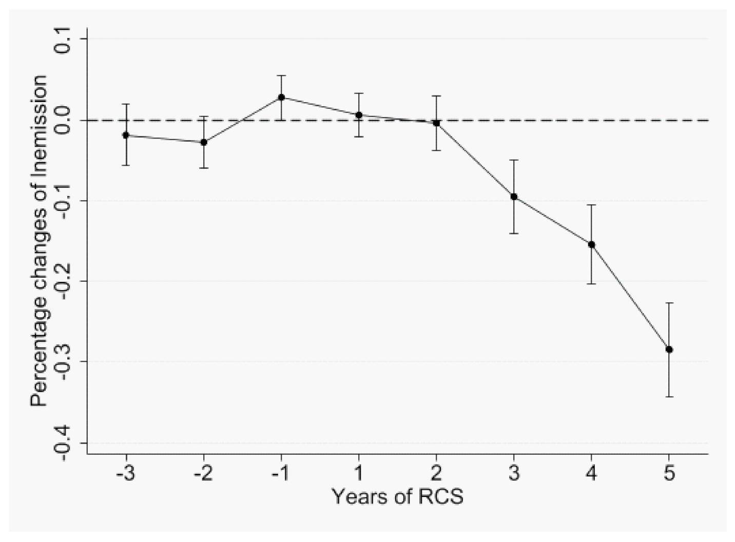
For the robustness of the estimation, we next verified whether the sample satisfied the parallel trend assumption [14]. We constructed the following regression model, as in the classic approach [15]:
where is and , is a dummy variable that equals 1 if it is the year before or after the implementation of the RCS, is a dummy variable that equals 1 if prefecture k is one of the pilot prefectures in the sample period, and and are fixed effects for the firm and year. If estimates of do not have a significant difference between the treatment group and the control group, the parallel trend assumption is satisfied.
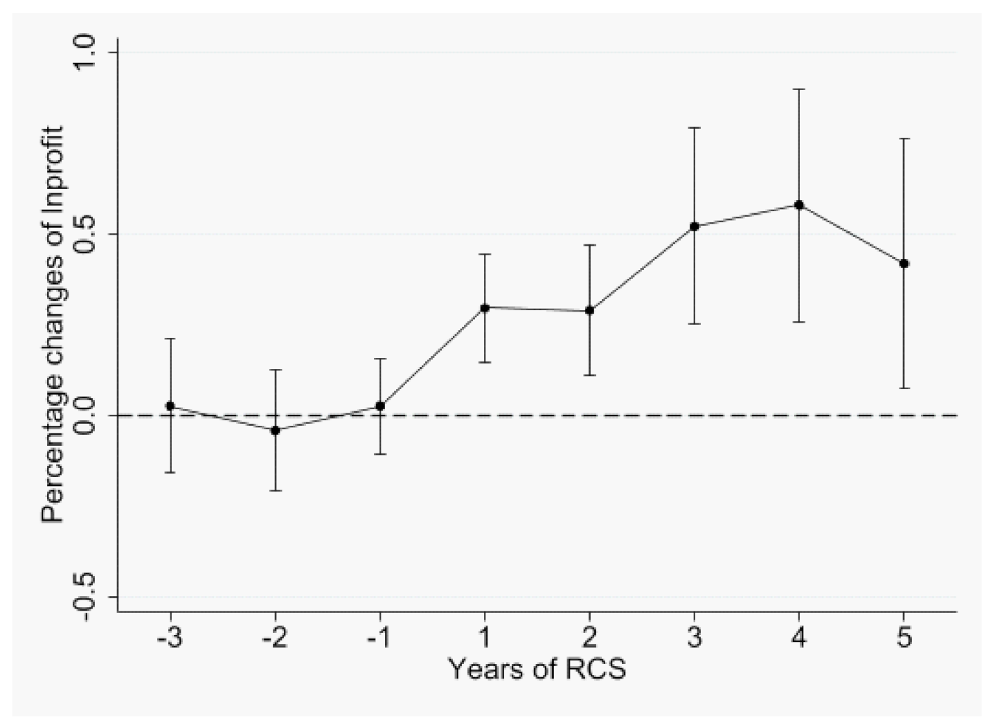
Figure 1 and Figure 2 illustrate the validity of our identification strategy. Figure 1 suggests that the time trends of the logarithms of the COD emissions of polluting firms in the treatment group and the control group were similar before the implementation of the RCS. However, after the implementation of the RCS, polluting firms in the treatment group showed a significant reduction in COD emissions. The firms’ profits before and after the implementation of the RCS in the two groups were similar.
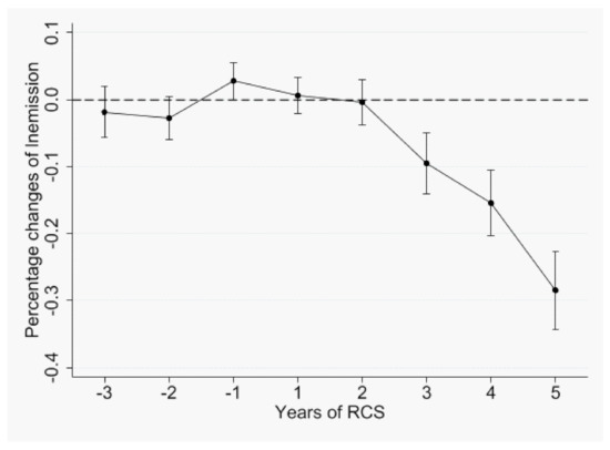
Figure 1.
Pre-existing COD emission trend.

Figure 2.
Pre-existing trend for profit.
Heterogeneity
This section explores the heterogeneous impacts of the RCS across firms of different industries, regions, ownership, and location. Heterogeneity may exist because of the difference in local governments’ regulations. For example, according to the extant literature, firms of different ownership are regulated differently [16]. Prefectures in different regions also implement regulation policies of different levels of stringency. According to the extant literature, the eastern provinces in China generally implement more strict emission regulations than other provinces [17]. At the industry level, heavily polluting industries are generally regulated more strictly [8]. From the angle of free-riding, much of the literature has found that pollution regulation is loose at provincial boundaries [9,10].
We started by investigating how the river chief system affected the COD emissions and profits of polluting firms in different industries. According to the extant literature, we categorized the 36 two-digit polluting industries into industries of heavy, moderate, and light pollution, as shown in Table 3 [18].
Table 3.
Industries classified by pollution level.
We next applied the regression model (1) to the three sub-samples of the heavily polluting, moderately polluting, and lightly polluting industries. Table 4 presents the results.
Table 4.
Industrial heterogeneity.
Obviously, the RCS significantly reduced the COD emissions in heavily polluting industries by 6.3%, while it significantly increased their profits by 5.5%. Both effects were significant at 1%. The other two industries also reduced their COD emissions, but the effect was not statistically significant. Firms in moderately polluting industries, on average, experienced an increase in profit by 2.5% after the RCS at the significance level of 5%, while the profits of firms in lightly polluting industries were not affected by the RCS. Table 3 confirms our conjecture about emission abatement—that local governments mainly targeted heavily polluting industries. It is also worth mentioning that, according to the Chow test, which is used to examine whether the true coefficients in two linear regressions on different datasets are equal, the percentage of profit increase in heavily polluting firms was larger than that in moderately polluting firms. The discrepancies in profits among industries indicate a possible transfer of the negative shock from RCS along the production line; on average, heavily polluting industries were located the furthest upstream on the production chain among the three industries, while lightly polluting industries were located the furthest downstream. As the extant literature suggests, environmental regulation can also affect the output price [19]. If the upstream industries have more bargaining power in determining the prices of intermediate inputs, their profits could increase, even with significant reductions in COD emissions. In contrast, it is generally more difficult for firms in lightly polluting industries to transfer the burden to consumers in the consumption market because consumption price stability has always been one of the main targets of the Chinese government. We will discuss the influencing channels through which the RCS affects firms’ profits in more detail in Section 4.
We next checked how the impacts of the RCS differed across regions by running the regression model (1) on the four sub-samples of eastern, northeastern, central, and western China based on the central government’s classification. Table 5 presents the results.
Table 5.
Regional heterogeneity.
The first observation is that the RCS generated a heterogenous effect across the regions. It significantly reduced polluting firms’ COD emissions in eastern China and northeastern China by 3.2% and 10% at the level of 5%, but it also significantly increased firms’ profits in the eastern provinces by 2.9% at the level of 1%. The Chow test verified that the emission abatement in the eastern provinces was larger than that in the northeastern provinces. In contrast, the RCS significantly increased polluting firms’ COD emissions in central and western China by 33% and 47% at the level of 1%, and it also increased firms’ profits in the central provinces by 8%. However, the magnitudes of the coefficients of emission in these two regions were not statistically different. This pattern confirms our conjectures that the eastern provinces put stringent regulations on emission abatement. (Because of the high population density and the high level of average income in eastern China, citizens are more concerned about their health than those in other regions of China. Hence, local governments’ incentives for environmental protection are also strong.) Moreover, consistently with the extant literature, the central and western provinces fit the “pollution paradise” hypothesis: Polluting firms tend to invest in the central and western provinces, where local governments emphasize economic development more, as compared to the local governments in the eastern provinces [5,20]. Despite the increase in COD emissions, the profits of polluting firms in the western provinces were not affected.
We next checked the possible heterogeneity with respect to enterprise ownership. Compared to private firms and foreign firms, state-owned firms usually gave higher priority to social responsibility than profit maximization, and could thereby be assigned more stringent abatement targets; however, political protection from local governments and the attempt to stabilize employment suggest that state-owned firms may receive less stringent regulations. Hence, the effect of the RCS on state-owned firms is ambiguous. Foreign firms primarily have advanced abatement technologies and, hence, a lower cost of emission abatement [21]. Private firms generally have no technological advantage compared to foreign firms, and they receive, on average, less political protection from local governments than state-owned firms do. Therefore, the negative impact of the RCS may be the largest for private firms. We ran the specification (1) on the three sub-samples of state-owned, private, and foreign firms, and the results are presented in Table 6.
Table 6.
Ownership heterogeneity.
As we anticipated, local governments’ conflict concerns for state-owned firms made the impact of the RCS on their emission abatement ambiguous; state-owned firms’ COD emissions were not significantly affected. Their profits increased by 11.7% at the significance level of 1%. Private firms and foreign firms reduced their COD emissions by 4.4% and 6.8%, respectively. Nonetheless, private firms’ profits were not affected, while foreign firms’ profits increased by 4.1% at the significance level of 1%. These results also confirmed foreign firms’ technological advantages. The Chow test verified that the emission abatement by foreign firms was larger than that by private firms and that the increase in the profits of state-owned firms was larger than that of foreign firms.
We next explored the free-riding incentive at provincial boundaries. Extant studies about water pollution reveal that, at provincial boundaries along a river, upstream firms face less stringent regulations than downstream firms [9,10]. Since some prefectures in Jiangsu province and Zhejiang province share the Tai Lake, we checked the emission behaviors at the provincial boundaries without identifying the “upstream” and “downstream” regions. Table 7 presents the regression results of the specification (1) on the two sub-samples: the sub-sample of firms located near provincial boundaries, defined as firms that were located in districts or counties at provincial boundaries, and the sub-sample of firms in the interior of a province [10].
Table 7.
Interior and provincial boundaries.
The RCS significantly reduced interior polluting firms’ COD emissions by 5.6% at the level of 1%, while it also increased their profits by 2.6% at the significance level of 1%. In contrast, the RCS did not affect the COD emissions of polluting firms at provincial boundaries, but it did increase their profits by 4.7%. The results regarding emission abatement at provincial boundaries verified the free-riding problem identified by previous studies. The Chow test also verified that the increase in profits of firms at provincial boundaries was larger than that of those in the interior.
To further explore the reason behind the above heterogenous results, we classified polluting firms in different regions by their levels of pollution. Because neither the COD emissions nor the profits of light-polluting firms were significantly affected by the RCS in any regions, we only present the results for heavily and moderately polluting firms in Table 8 and Table 9.
Table 8.
Regional × industry heterogeneity: COD emissions.
Table 9.
Regional × industry heterogeneity: profit.
The first observation from Table 8 is that provinces in different regions appeared to assign the abatement tasks to different industries after implementing the RCS. Eastern provinces focused on heavily polluting industries, while northeastern provinces and central provinces focused on moderately and lightly polluting industries, respectively. Heavily and moderately polluting industries in the RCS pilot prefectures of the central provinces increased their COD emissions significantly. In the RCS pilot prefectures of the western provinces, firms of moderately polluting industries increased their COD emissions, and the magnitude was statistically larger than that of firms in the central provinces according to the Chow test.
Table 9 indicates that in the eastern provinces, only heavily polluting industries’ profits were significantly affected by the RCS, despite the significant emission abatement; the profits increased by 5.1% at the significance level of 1%. Similarly, in the northwestern provinces, firms in moderately polluting industries managed to increase their profits by 5.1% despite the emission abatement. Although firms in heavily and moderately polluting industries in the central provinces increased their COD emissions, only firms in moderately polluting industries experienced an increase in profits. This increase, however, was not statistically different from the increase in profits of moderately polluting firms in the northeastern provinces.
We next classified polluting firms of different ownership types by their levels of pollution. Table 10 and Table 11 present the results.
Table 10.
Ownership × industry heterogeneity: COD emissions.
Table 11.
Ownership × industry heterogeneity: profit.
Table 10 indicates that the COD emissions of state-owned firms were not affected by the RCS, regardless of the industry. In heavily polluting industries, emission abatement of private firms and foreign firms contributed the most to the results of the full sample in Table 4. However, state-owned and foreign firms in heavily polluting industries in the pilot prefectures increased their profits, which is consistent with Table 6. However, the magnitudes of the two coefficients were not statistically different.
We finally investigated how the RCS affected interior and boundary firms of different pollution levels. The results are presented in Table 12 and Table 13.
Table 12.
Location × industry heterogeneity: COD emissions.
Table 13.
Location × industry heterogeneity: profit.
Interior firms in the heavily polluting industries of the pilot prefectures managed to reduce the COD emissions and increase the profits, which is consistent with Table 4. Heavily polluting firms of the pilot prefectures on provincial boundaries experienced an increase in profits without reducing their COD emissions, which is consistent with Table 7. Interior firms in moderately polluting industries managed to increase their profits by 2.7%. In lightly polluting industries, interior firms reduced their emissions while their profits were not significant affected. Boundary firms did not change their COD emission levels, but increased their profits by 8%. This was the only case in which firms in lightly polluting industries increased their profits.
4. Discussion: Mechanism
While the differences in firms’ emission abatement are generally consistent with our conjecture, an interesting yet puzzling result in the empirical analysis is that the reduction of COD emissions in heavily polluting industries following the implementation of the RCS led to an increase in their net profits. In this section, we explore several channels through which the RCS may have caused this result, including: (1) an increase in the gross revenue of production, measured by the total output value of manufacturing; (2) a reduction in the production cost caused by efficient cost management, measured by the increase in the capital–output ratio; (3) a reduction in the production cost caused by a decrease in employment (the wage data are not available); (4) an increase in the amount of government subsidies; (5) innovation, measured by the increase in the output value of new products; (6) a decrease in market competitiveness, measured by an increase in the Herfindal–Hirtch Index of the top eight firms—HHI 8. (The Lerner index and the gross revenue of the main business can also be used to measure the market competitiveness. However, the two measures both have the issue of endogeneity.)
We replaced the dependent variable in the specification (1) with measures of the six possible channels and present the results in Table 14. (Because employment was also used as a control in the basic regression, we removed it when the dependent variable was the log of the total employment in Table 13).
Table 14.
Possible channels.
Both the gross revenue of production and the output value of new products significantly decreased, suggesting that these two channels cannot lead to an increase in profits. Similarly, we can rule out the decrease in employment as a possible channel. The capital–output ratio and the amount of government subsidies were not affected by the RCS policy. The significant increase in HHI is consistent with the observation in Table 2 that polluting firms’ profits increase. The rise in market concentration may have been caused by a larger reduction of output of small firms on average than that of large firms. It is worth noting that because only non-state-owned firms with fixed assets of more than 5 million RMB are included in the ASIFs (which increased to 10 million RMB after 2011), the increase in HHI may even have been underestimated. (Many pilot prefectures chose to shut down factories that produced visible or smelly wastewater. For example, according to the People’s Daily, until December of 2016, the pilot prefectures of Zhejiang Province shut down over 30,000 small factories and 50,000 farms.) The extant literature also emphasizes that shutting down small heavily polluting firms was a usual strategy in local governments’ environmental regulation of water pollution [8]. This could also explain why firms in heavily and moderately polluting industries in the central and western provinces increased their COD emissions after the implementation of the RCS; the total COD emissions in a prefecture could still decrease if small factories were forced to shut down. The emission abatement at the prefectural level after the implementation of the RCS is also confirmed by other studies [2].
We next check these channels according to the industries to investigate possible heterogeneity and present the results in Table 15.
Table 15.
Channels by industry.
Firms in all three industries experienced a significant reduction of output value, with the Chow test showing that the magnitude was the smallest in heavily polluting firms. Recalling that firms in heavily polluting industries also significantly reduced their COD emissions, the decrease in the total output value may have partly been caused by the reduction of the output quantity. The capital–output ratio of firms in heavily polluting industries increased at a significance level close to 10%, indicating a decrease in the efficiency of cost management, which was probably caused by the increased expenditure on emission abatement and the reduction in the output. Firms in heavily polluting industries also received fewer subsidies after the implementation of the RCS at the significance level of 1%, while firms in lightly polluting industries received more subsidies at a significance level close to 10%. This result points to an interesting possibility—that local governments may be aware of the transfer of the negative shock along the production line.
Firms’ total employment significantly increased in all industries, while the Chow test suggested that the largest magnitude of this effect occurred in lightly polluting firms. Firms’ output values of new products significantly decreased in all industries. The Chow test verified that the magnitude of this negative effect was the smallest in heavily polluting industries and the largest in lightly polluting industries. The HHI also significantly increased in the three industries, and heavily polluting industries had the largest magnitude according to the Chow test.
Overall, these results suggest that the increase in net operating profits of firms in heavily polluting industries is mainly caused by the increase in the market concentration. This gives leading firms more bargaining power in determining the contractual prices. On the other hand, although firms in lightly polluting industries received more subsidies and experienced a slight increase in HHI after the implementation of the RCS, their profits were not affected. This result was mainly caused by the lack of innovation, which was reflected by the huge drop in the total sales of new products. In addition, compared to firms in heavily polluting industries, firms in lightly polluting industries may have insufficient bargaining power in determining prices and transferring the negative shock to consumers.
5. Robustness
We first replaced COD with another hazardous pollutant: ammonia nitrogen (NH-N). The coefficients of the RCS in all regressions were qualitatively the same as before, except for some differences in the significance level. We also replaced the net operating profit with the net total profit and achieved qualitatively the same results. The results of the basic regression (1) are reported in the first two columns of Table 16. The rest of the results on heterogeneity are reported from Tables S1–S4 in Supplementary Materials.
Table 16.
Robustness.
We next checked whether different ways of clustering the standard error could affect our regression results. Under the industry–year cluster, the implementation of the RCS remained, except that its impact on lightly polluting industries also became significant. The results of the basic regression (1) are reported in columns (3) and (4) of Table 16. The rest of the results on heterogeneity are reported from Tables S5–S8 in Supplementary Materials.
We also conducted a counter-factual analysis that assumed that the pilot prefectures implemented the RCS two years before the actual time. The results are reported in columns (5) and (6) of Table 16. The coefficients in the counter-factual analysis are not significant, indicating that except for the shock of the RCS, no systematic difference exists between the treatment group and the control group.
6. Concluding Remarks
The novel river chief system is a decentralized policy for water protection in China, which does not involve the central government setting precise targets for improvement of water quality. Hence, investigating its firm-level impact on polluting firms in pilot prefectures is necessary for the understanding of the operation of the RCS and the resulting implications. In this paper, we used a generalized DID method to explore the impact of the RCS on polluting firms’ COD emission abatement, the net operating profits, and the heterogeneity. We found that heavily polluting industries received the most stringent regulations on average, as their emissions were reduced by 6.3 percent, while the moderately and lightly polluting industries did not reduce their emissions. However, heterogeneity existed across regions. After the implementation of the RCS, the eastern provinces contributed the most in terms of emission abatement; polluting firms, on average, reduced emissions by 3.2 percent, which, again, was mainly caused by firms in heavily polluting industries. In contrast, the firm-level emissions in the central and western provinces even increased. Across enterprise ownership types, non-state-owned firms contributed to emission abatement in all industries; private firms reduced emissions by 4.4 percent, and foreign firms reduced emissions by 6.8 percent. However, state-owned firms did not significantly reduce emissions. The free-riding incentive at provincial boundaries also existed; polluting firms near provincial boundaries were not affected by the RCS, while those in the interior of a province significantly reduced COD emissions by 5.6 percent.
Interestingly, emission abatement did not lead to a reduction of the net profits, especially in heavily polluting industries in the eastern provinces, which contributed the most to emission abatement; their emissions were reduced by 6.1 percent, but their profits also increased by 5.1 percent. In contrast, regardless of the enterprise ownership, profits of firms in lightly polluting industries in all provinces were not affected. While we suspect that these results were caused by a transfer of the cost burden from the negative shock generated by the RCS along the production line, a detailed investigation of the mechanism verifies this conjecture to some extent. The rise in market concentration is the only channel through which the RCS can increase the profits of firms in heavily polluting industries. This positive effect is sufficiently strong to outweigh the negative effects generated by the other five channels.
Our results provide rich policy implications for the enforcement of the RCS. First, local governments should consider the fact that the stringent regulations imposed on firms in heavily polluting industries can create negative effects on firms in lightly polluting industries that are located relatively downstream on the production line. Second, innovation activities are negatively affected in all industries, suggesting that the RCS policies are executed with some economic costs. Third, the central government may evaluate the economic benefit and cost of polluting firms’ increased emissions in the central and western provinces of China to determine whether extra supervision is necessary.
Supplementary Materials
The following supporting information can be downloaded at: https://www.mdpi.com/article/10.3390/su14063418/s1, Table S1: Emission and profits by industry, Table S2: Emission and profits by region, Table S3: Emission and profits by enterprise ownership, Table S4: Emission and profits by location, Table S5: Emission and profits by industry, Table S6: Emission and profits by region, Table S7: Emission and profits by enterprise ownership, Table S8: Emission and profits by location.
Author Contributions
Conceptualization, X.X. and Y.C.; methodology, X.X. and Y.C.; software, Y.C. and X.M.; validation, X.X. and X.M.; formal analysis, X.X. and Y.C.; investigation, Y.C.; resources, X.M.; data curation, X.M.; writing—original draft preparation, X.X.; writing—review and editing, X.M.; visualization, Y.C.; supervision, X.X.; project administration, X.X. All authors have read and agreed to the published version of the manuscript.
Funding
This research received no external funding.
Institutional Review Board Statement
Not applicable.
Informed Consent Statement
Not applicable.
Data Availability Statement
Not applicable.
Acknowledgments
We thank Weisi Xie, Jing Tan, and the anonymous reviewers for their insightful comments and suggestions. All errors are our own.
Conflicts of Interest
The authors declare no conflict of interest.
References
- He, G.; Wang, S.; Zhang, B. Watering Down Environmental Regulation in China. Q. J. Econ. 2020, 135, 2315–2385. [Google Scholar] [CrossRef]
- She, Y.; Liu, Y.; Jiang, L.; Yuan, H. Is China’s River Chief Policy effective? Evidence from a quasi-natural experiment in the Yangtze River Economic Belt, China. J. Clean. Prod. 2019, 220, 919–930. [Google Scholar] [CrossRef]
- Liu, H.; Chen, Y.; Liu, T.; Lin, L. The River Chief System and River Pollution Control in China: A Case Study of Foshan. Water 2019, 11, 1606. [Google Scholar] [CrossRef] [Green Version]
- Caudaua, F.; Dienesch, E. Pollution Haven and Corruption Paradise. J. Environ. Econ. Manag. 2017, 85, 171–192. [Google Scholar]
- Dou, J.; Han, X. How does the Industry Mobility Affect Pollution Industry Transfer in China: Empirical Test on Pollution Haven Hypothesis and Porter Hypothesis. J. Clean. Prod. 2019, 217, 105–115. [Google Scholar] [CrossRef]
- Shen, K.; Jin, G. The Policy Impact of Local Governments’ Environmenal Regulation in China: A Study Based on the Development of the River Chief System. Soc. Sci. China (In Chinese). 2018, 2018-5, 92–115. [Google Scholar]
- Li, J.; Shi, X.; Wu, H.; Liu, L. Trade-off between Economic Development and Environmental Governance in China: An Analysis Based on the Effect of River Chief System. China Econ. Rev. 2020, 60, 101403. [Google Scholar] [CrossRef]
- Wang, C.; Wu, J.; Zhang, B. Environmental Regulation, Emissions and Productivity: Evidence from Chinese COD-emitting Manufacturers. J. Environ. Econ. Manag. 2018, 92, 54–73. [Google Scholar] [CrossRef]
- Kahn, M.; Li, P.; Zhao, D. Water Pollution Progress at Borders: The Role of Changes in China’s Political Promotion Incentives. Am. Econ. J. Econ. Policy 2015, 7, 223–242. [Google Scholar] [CrossRef] [Green Version]
- Cai, H.; Chen, Y.; Gong, Q. Polluting thy Neighbor: Unintended Consequences of China’s Pollution Reduction Mandates. J. Environ. Econ. Manag. 2016, 76, 86–104. [Google Scholar] [CrossRef]
- Chen, Z.; Kahn, M.; Liu, Y.; Wang, Z. The Consequences of Spatially Differentiated Water Pollution Regulation in China. J. Environ. Econ. Manag. 2018, 88, 468–485. [Google Scholar] [CrossRef]
- Brandt, L.; Van Biesebroeck, J.; Zhang, Y. Creative accounting or creative destruction? Firm-Level productivity growth in Chinese manufacturing. J. Dev. Econ. 2012, 97, 339–351. [Google Scholar] [CrossRef] [Green Version]
- Heyman, F.; Sjoholm, F.; Tingvall, P. Is There Really a Foreign Ownership Wage Premium? Evidence from Matched Employer–employee Data. J. Int. Econ. 2007, 73, 355–376. [Google Scholar] [CrossRef] [Green Version]
- Galiani, S.; Gertler, P.; Schargrodsky, E. Water for Life: The Impact of the Privatization of Water Services on Child Mortality. J. Political Econ. 2005, 113, 83–120. [Google Scholar] [CrossRef] [Green Version]
- Beck, T.; Levine, R.; Levkov, A. Big Bad Banks? The Winners and Losers from Bank Deregulation in the United States. J. Financ. 2010, 65, 1637–1667. [Google Scholar] [CrossRef] [Green Version]
- Pargal, S.; Wheeler, D. Informal regulation of industrial pollution in developing countries: Evidence from Indonesia. J. Political Econ. 1996, 104, 1314–1327. [Google Scholar] [CrossRef]
- Chen, B.; Cheng, Y. The Impacts of Environmental Regulation on Industrial Activities: Evidence from a Quasi-natural Experiment in Chinese Prefectures. Sustainability 2017, 9, 571. [Google Scholar] [CrossRef] [Green Version]
- Wang, J.; Liu, B. Environmental regulations and Firms’ TFP: An Empirical Analysis Based on Chinese Manufacturing Firms. China Ind. Econ. 2014, 2014, 44–56. (In Chinese) [Google Scholar]
- Greenstone, M.; List, J.; Syverson, C. The Effects of Environmental Regulation on the Competitiveness of U.S. Manufacturing. NBER Working Paper 18392. 2012. Available online: https://ideas.repec.org/p/nbr/nberwo/18392.html (accessed on 15 February 2022).
- Yin, J.; Zheng, M.; Li, X. Interregional Transfer of Polluting Industries: A Consumption Responsibility Perspective. J. Clean. Prod. 2016, 112, 4318–4328. [Google Scholar] [CrossRef]
- Lanjouw, J.; Mody, A. Innovation and the International Diffusion of Environmentally Responsive Technology. Res. Policy 1996, 25, 549–571. [Google Scholar] [CrossRef]
Publisher’s Note: MDPI stays neutral with regard to jurisdictional claims in published maps and institutional affiliations. |
© 2022 by the authors. Licensee MDPI, Basel, Switzerland. This article is an open access article distributed under the terms and conditions of the Creative Commons Attribution (CC BY) license (https://creativecommons.org/licenses/by/4.0/).