Monetary Policy, External Shocks and Economic Growth Dynamics in East Africa: An S-VAR Model

Abstract

Resulting from the incessant political and economic uncertainty that bedevils the EAC region in the recent past, the various governments have used monetary policy changes in response to shocks from macroeconomic variables. However, the available literature shows a non-agreement by scholars as far as the dynamics in monetary policy, external shocks and macroeconomic activity connections are concerned, for both country-by-country analyses and regional assessments. This article widens the frontiers of knowledge about how the dynamics of monetary policy, external shocks and macroeconomic performance interact within the EAC economic region. We adopted the S-VAR method because of its contemporary nature as far as a transmission of monetary policy approach is concerned. The interconnectivity among the countries of EAC is an indication that any shock to the price of commodities (non-oil commodities) has significant implication on the exchange rate, which will be channelled through the supply of money and monetary policy to the GDP. The need to diversify the productive and export base of member countries, compared to the continuous dependence on one or a few products as the major source of income, is hereby advocated.

1. Introduction

One of the leading economic regions in sub-Saharan Africa is the East Africa Community (EAC), with the European Union countries being its major trading partners [1]. Predominantly, the region depends largely on primary products whose prices are subject to external shocks and, as such, had resulted in monetary policy dynamics and macroeconomic instability in the past [1,2,3]. This suggests that the economic activities of the region, just like other regions within the sub-Saharan Africa, including production of goods and services, have been at the mercy of external shocks arising from unstable prices of oil and commodity products [4,5,6].

Among other things, the aim of the Intergovernmental Authority on Development (IGAD) was to open the countries within the EAC to the outside world, especially regarding trade. According to [7] SADC constitutes the greatest trading partner with EAC during the period of 1995–2012. In the United Nations Conference on Trade and Development (UNCTAD) report of 2018, trade composition of the EAC has also changed from the erstwhile dominance by European markets to other sub-Saharan countries and the developing Asian countries. It was further reported that EAC trading activities with SSA rose from 30% in 2004 to 36% by the end of 2012. Similarly, the share of exports to Asia from EAC rose from 17% to 26% during the same period. Studies by [8,9] have emphasized the relevance of intra-regional trade as a major avenue by which the consequences of external shocks can be alleviated. In essence, the theory of Optimum Currency Area (OCA) as an ingredient of economic integration can ameliorate the incidence of shocks from commodity prices. In a study that assessed the benefits of trade integration among the countries of EAC, full implementation of common market protocols and customs unions were proffered by [9] for a successful common currency by member countries. Consequently, the proposed East African Monetary Union, aiming at adopting a single currency by the countries of the region in the year 2024, could be a step in the right direction.

Nonetheless, price volatility arising from supply shocks (bubble or burst) and the secular variations in real commodity and oil prices, coupled with the attendant losses in terms of trade, have affected the foreign exchange earnings, investment, indebtedness, poverty and other macroeconomic activities of the region [1], leading to monetary policy manipulations. The EAC was launched in 2000 whereas the treaty had earlier been signed in 1999 by the three countries (Kenya, Tanzania and Uganda) that initiated its establishment. Among other things, this treaty recognized the need to establish sister unions in the areas of customs, monetary and a unified market that will guarantee a future federating entity for the community. To pave the way for its smooth take-off in 2010, the customs union was inaugurated in 2005. Furthermore, to also ensure unhindered movement of human resources, capital, goods and services, governments of the constituting countries signed the common market alliance in 2009. Not only that, the enforcement and monitoring of the macroeconomic aggregate of the region and the negotiating procedure through legal, monetary outlook and institutional structures were put into consideration in 2010. To promote the participation of other countries, Burundi and Rwanda were accommodated as members in 2007. In all, economic advancement of the region arising from the above activities requires a monetary policy package that will not only create conducive regional integration but also ensure faster and economic emancipation. Countries within the EAC are categorized as Highly Indebted Poor African Countries and the persistent changes in policy formulation and implementation were the consequences of external shocks in the form of price variations and macroeconomic instability. For instance, the 2007–2009 global financial crisis and the bubbles that followed thereafter took their toll on the macroeconomic activities of both the oil- and commodity-dependent economies. As reported by [6,10], the decrease in commodity prices in the African continent (East Africa inclusive) in recent times has put doubt in the minds of economic analysts on the growth yearnings and the possibility of poverty reduction across the continent. It was further advanced that macroeconomic variables such as the exchange rate policy will play an important role in revamping the likely effects of commodity and oil price variations in the region.

The East Africa subregion of the sub-Saharan Africa is predominantly dependent on primary commodity exports, whose prices are subject to external dictation. Burundi has coffee, cotton, hides, sugar and tea as her major commodity exports. According to [4], coffee accounts for 36.4% of the GDP of Burundi while the major exports for Uganda are coffee, cotton, flowers, fish and fish products, gold, horticultural products and tea. For Tanzania, cashew nuts, coffee, cotton and gold are its major exports, while Kenya exports cement, coffee, fish, horticultural products, petroleum products and tea. Furthermore, Kenya, which is the largest economy of the region, produces in large quantity, such that shocks to the oil price in international markets adversely affect the local production of goods and services. Nonetheless, the fall in global commodity prices coupled with the current global COVID-19 pandemic in no small way adversely affected the terms of trade in the region. Not only that, as oil importing nations, local production of the region is a function of oil price volatilities. Thus, the effect of oil price vagaries is expected to be more pronounced within the region. Furthermore, resulting from the incessant political and economic uncertainty that has bedevilled the region in the recent past, the East Africa sub-regional governments made monetary policy changes in response to shocks from some identified macroeconomic variables. As raw agricultural commodity exporters for foreign exchange earnings (tea, coffee, cut flowers, fish, tobacco and vegetables), countries of the region also import energy in the form of oil as input. For instance, Kenya and Ethiopia produce tea and coffee, respectively; the United Republic of Tanzania produces cashews; and Uganda produces coffee—all of these in commercial quantities. These raw products constitute a higher percentage of the GDP of the EAC as a region [5,11]. However, the available evidence shows that production of goods and by extension services cannot be divorced from energy resources such as oil [12,13]. In essence, shocks from oil prices will not only affect commodity outputs but also the prices in international markets. With the European Union (EU) as the major trading partners of EAC, the macroeconomic activities of the region are affected by changes in commodity prices whose prices are susceptible to external shocks and, consequently, monetary policy manipulations.

Nevertheless, mixed reactions have trailed the discussions around the relationship between the combined influence from changes in monetary and fiscal policies on macroeconomic variables [14,15,16,17,18]. Buyukbasaran et al. (2020) used Bayesian S-VAR in examining how shocks from monetary policy and fiscal policy influenced a few macroeconomic variables for Turkey and confirmed the mixed reactions. On one hand, the response of the shocks from both policies to demand and supply shocks jointly complement each other, while, on the other hand, individual policy responds separately in form of a substitute to shocks from demand and supply. In essence, the effect of loosed or contractionary monetary and fiscal policies on the shocks from demand and supply are complementary, whereas the effect would be substitute if one of the policies is loosed such that the other is contractionary. These reactions will make it possible for the unanticipated shocks to be investigated rather than the anticipated shocks.

In this study, we focused on two major objectives. The first one explored the external shocks, macroeconomic performance and endogenous determinants of monetary policy dynamics within the EAC, while the second is an impact analysis of these economic indices in relation to monetary policy dynamics using the S-VAR method of estimation. The five selected countries are Burundi, Kenya, Rwanda, United Republic of Tanzania and Uganda, while our variables of concern are monetary policy dynamics (dependent variable), interest rate, money supply, gross domestic product growth rate, exchange rate, net domestic credit, inflation, oil and variations in the price of commodities. Research of this nature has become imperative and of interest for monetary and economic policy managers in East Africa, who must know the endogenous determinants of monetary policy within the region and the impact of these factors in correlation with monetary policy.

Theoretical Framework (Monetary Transmission Mechanism)

Traditionally, the main objectives of monetary policy are to maintain price stability, control money supply, achieve economic growth, employment generation and, by extension, nominal GDP [19,20,21]. The means and extent to which monetary policy affect economic activities is referred to as the monetary transmission mechanism (MTM). Four major channels have been identified through which monetary policy decisions affect economic activities in an economy [22]. These are the direct interest rate effects, which affect not only the cost of credit to borrowers but also the flow of cash of both borrowers and lenders. This channel remains the most effective and commonest means by which the effect of monetary policy is transmitted in an economy. From an expansionary monetary policy stance, the interest rate is reduced while investment and consumption spending would increase [23]. These will enlarge the aggregate demand and increase the general output. The second is the exchange rate channel. As a result of the increase in supply of money arising from a reduction in the interest rate, denominated local assets are cheaper relative to foreign goods because of local currency depreciation; therefore, the net exports and output would increase [24]. The third is through its effects on the prices of local assets such as stock markets, bonds and prices of real estate. Most important is the stock prices according to Tobin’s q investment theory. Lastly is the availability of a credit channel through bank lending and balance sheet channels. One major challenge of this mechanism is agency issue through asymmetry information distortion [25]. Some monetary policy instruments through which monetary authorities exert policy effects in an economy include the interest rate, money supply, exchange rate manipulation and control of inflation. Therefore, the starting point in the discussion about the interaction between the identified monetary policy instruments is the baseline model. This model was extended by incorporating other relevant variables, such as the exchange rate [20]. Furthermore, since the countries under investigation are integrated economically, which make them susceptible to external shocks through import prices, we consider it necessary to examine the explanatory power of the main external variables in addition to the exchange rate and other monetary policy instruments. To this end, commodity and oil price volatilities were incorporated into the Structural VAR model to capture their effects and interactions with other variables.

2. Literature Review

The EAC region has received less attention in the economic literature as a commodity-dependent economy bloc. Related regional studies include [4,15,26,27]. The outcome of the S-VAR model by [15] showed the existence of heterogeneity in magnitude and directions of macroeconomic responses to commodity price shocks in Africa. Addison et al. (2016) employed a structural non-linear dynamic model for some selected SSA countries, with the resolution that unexpected external shocks to agricultural outputs have no effect on the per-capita income of the continent. The few country-specific studies in this area include [6] for Zambia, [22] for Thailand, [28] for Ghana and [29] for South Africa. In all, none of these studies synchronized the implications of shocks from the prices of oil and commodity viz-a-viz macroeconomic dynamics, either as a time series or panel data investigation. In this article, the aim is to widen the frontiers of knowledge about the interactions in the dynamism of monetary policy, external shocks and macroeconomic performance of the EAC, using the Structural Variance Auto-Regressive method.

Various degrees of commodity shocks to output and business cycles/terms of trade have been identified in the literature such that the differences in model application account for the different results from those studies [30,31,32,33]. Roch (2019) adopted the Panel-SVAR on 22 commodity-exporting countries in an investigation about how shocks in commodity terms of trade affect those countries’ business cycles. The study, which covers 1980–2017, did not only reveal a substantial effect of commodity price shocks to the business cycles of the selected countries but also recorded a higher percentage of 30% in terms of how commodity terms of trade influence the business cycles of those countries. This was a clear deviation from existing studies that recorded at highest a 10% influence. Similar studies, such as those by [33,34], employed different methodologies and data variation in their separate studies about how the manufacturing section of the economy influenced GDP and concluded that what matters most is the channels of the policy transmission mechanism among policy variables. Schmitt-Groh’e and Uribe (2017) recorded a rate of less than 10% influence in the trade shock to output in their investigation about how the terms of trade interact with economic activities, using S-VAR for 38 countries. Authors such as [35] reported for Vietnam that some monetary policy variables, which include interest rate, supply of money and domestic credit, played important roles in controlling inflation in that country. Specifically, domestic credit and supply of money exhibit a greater influence on inflationary pressure during the period under investigation. The study, which spanned from 2005 to 2017, further revealed that shocks from monetary policy vary from time to time, depending on the combination of instruments used and effects of global financial disturbances. A similar study but with varying variables was done by [36], where interest rate was seen as an effective tool for regulating the inflation rate in Romania. According to [37] exchange and interest rates served as efficient monetary instrument in upholding the GDP for Romania. In all, these monetary variables interact to achieve one policy objective or the other.

Shocks from monetary policy was further tested on the behaviours of the stock market activities in some African countries by [38]. The study included supply of money, real interest rate and inflation as policy variables in a Panel-VAR model and revealed a symbiotic association among monetary policy and stock exchange activities. Antwi et al. [28] and Akosah et al [39] examined the interactions between inflation, exchange rate, output, rate of interest and money supply in Ghana and concluded that the apex bank’s reactions to these economic variables depend on the perceived policy targets. In their investigation on the effects of some macroeconomic variables on the exchange rate in Ghana, Antwi et al. [28] showed that money supply, inflation and interest rate indirectly influenced the exchange rate. The panel study by [40] on CEMAC and the UEMOA CFA zone revealed that monetary policy instruments influence GDP in the short run and not in the long run. As a way forward to encourage investors, both studies canvassed for reductions in money supply and interest rates if inflation is to be brought to the barest minimum. According to [41] the need to jealously guide monetary policy instruments in the cause of ECOWAS monetary integration has become imperative because of shocks on the GDP growth rate of that region.

Furthermore, Omojolaibi and Egwaikhide [42] employed Panel-VAR to examine the extent to which variation in the price of oil could impact economic activities in five oil-producing countries in Africa and discovered that the channel through which oil price variations affect macroeconomic activities in those countries was gross investment. Whereas variables such as real GDP, money supply and fiscal policy exert no significant influence on the volatility of oil price. In the same spirit, Addison et al [4] selected nine sub-Saharan African countries whose major income is from a single or few commodities, using structural nonlinear model, and submitted that a price increase or decrease in their agricultural products have an insignificant effect on the per capital income of those countries—an indication that the relationship is asymmetric in nature. The above findings vary compared to those of [4], where the implication of a shock from the price of oil to macroeconomic variables in oil-producing African countries differ. As an oil-importing country, Etornam [43] also employed the restricted VAR technique in their investigation about the nexus between shocks from the price of oil and some selected macroeconomic variables for Ghana and came up with a nonlinear association in shocks from the price of oil and those variables. In South Africa, the result of the S-VAR by [44] showed a trend of adverse implications due to the variations in the price of oil on the economic activities of the country. Variations in commodity prices posit a major challenge to the macroeconomic stability of African countries (East Africa inclusive), but the effect depend largely on an individual country’s structural characteristics and response to policy implementation [5]. In essence, the effects are not uniform but a function of procyclical or countercyclical consequences. While shedding more light on the nexus between commodity price fluctuations in some commodity-dependent African countries, the result of the structured VAR and descriptive analysis by [5] showed a heterogeneous relationship between shocks from commodity products and economic activities of the countries under investigation. Aligning with this was the study by [13] in Nigeria, using the S-VAR technique of estimation. The study concluded that shocks from oil price affect output and growth significantly and negatively.

Nonetheless, Dillon and Barrett [2] itemized three ways by which the price of commodity maize could be affected by external shocks and concluded that global oil price shocks affect maize outputs more than changes in the prices of maize in the global market. In-addition [45] admitted that the influence of some macroeconomic variables in shaping the direction and success of the proposed East Africa Monetary Union cannot be underestimated. The study employed the static and dynamic methods of estimation for five selected countries within the EAC zone and reported that shocks from exogeneous variables led to an upward inflationary level and a reduction in the GDP growth rate. Further, Buigut [46] concluded that interest rate was a weak instrument of monetary policy in Kenya, Tanzania and Uganda in a study that employed a three-variable recursive VAR approach. According to this study, no statistical implication was noted for real output or inflation as a result of changes in the rate of interest. Additionally, Abuka et al [47] reported that tight monetary policy did not only lead to loan application rejection by banks in Uganda but also reduced credit availability to borrowers, which then affected her economic activities. This confirmed an earlier suggestion by [48] where Uganda was advised against over dependence on monetary policy as a means of achieving some macroeconomic objectives since this could be counterproductive. In [49], it was revealed that the main channel through which the influence of monetary policy could be transmitted to inflation was the rate of interest in Kenya. Nonetheless, Ayubu [50] also confirmed inflation as real factor rather than monetary issue in a study that investigated the significance of the monetarists’ assertion about what money does during an inflationary period in Tanzania.

In Kenya, the study by [3] about monetary and fiscal policies’ implications on GDP suggested a systematic adjustment by monetary policy to deviation in fiscal policy from sustainable long-run economic growth. In another study, Wetite [51] revealed that monetary policy is more potent on economic growth than fiscal policy in a study on the relative effectiveness of both policies in Ethiopia. This was in contrast to [52], who showed fiscal policy as having more effects on growth than monetary policy in Ethiopia. Further attempts in the investigation about the association between the dynamics in monetary policy and GDP in the EAC region include those of [53,54,55]. Three VAR approaches, namely, Factor-Augmented, Bayesian and Structural, were employed by [53] while studying the dynamics in monetary policy influence for Burundi, Kenya, Rwanda, Tanzania and Uganda, with the conclusion that an adverse change in interest rate have a noticeable and favourable contribution in Burundi, Kenya and Rwanda but not in Tanzania and Uganda. Commenting on the formation of a monetary union for the EAC, Caporale and Gil-Alana [56] opined that monetary policy instruments have some roles to play in the proposed integration. This is an indication that macroeconomic activities within the region in relation to monetary policy variations are interwoven. On the contrary, Twinoburyo and Odhiambo [55] studied the linkage in monetary policy and GDP in Kenya and came with a neutral relationship outcome. Hence, investigating the dynamisms in monetary policy, external shocks and macroeconomic activities seems to be an interesting research area in view of the yet-to-commence monetary union for the EAC.

A comparative analysis of how exchange rate affected the manufacturing sector’s products and the transmitting apparatus of monetary policy in Libya and Nigeria was the aim of the study by [57]. The outcome of the structural variance decomposition approach was mixed, in that the exchange rate influence on growth in Nigeria was more pronounced than in Libya. Accounting for this could be the differences in the exchange rate management by both countries. While Nigeria operated a flexible exchange rate, Libya adopted a fixed operational system. Dilion and Barrett (2015) asserted that one staple commodity within the EAC economic region is maize whose price is often affected by oil price changes and transportation costs. They further observed that with the underdeveloped nature of the transportation system of the region, coupled with shocks from oil price input, the macroeconomic activities of the region are expected to be unstable. The available literature clearly shows that opinions differ on the relationship between the monetary policy dynamics, external shocks and macroeconomic activities for both country-by-country analyses and regional assessments. Not only that, but it was further established that interest rate, money supply, net domestic credit, exchange rate, GDP growth rate and volatilities in oil and commodity prices constitute the relevant variables of concern; thus, the model specifications in this study were based on them. These variables have been identified as factors affecting monetary policy dynamics, especially at regional levels [40,57,58,59].

3. Data and Methods

3.1. Definition of the Variables and Sources

The study is based on unbalanced panel data, sourced mainly from World Development Indicators (WDI) for the period 1980–2019. A comprehensive description and measurement of the interested variables are presented in the following

Table 1. Definition, Measurement and Variables Sources of Data.

Variable	Description	Measurement	Sources of Data
Real GDP growth rate	This is the growth rate value of total annual output of goods and services produced in the economy in a particular period of time usually a year. It is used as proxy for Economic Growth (see Nogueira 2009)	It is measured in percentage and as the value of all productive resources that nations used in a year after correcting for inflation. This implies that real GDP is the value of nominal GDP that has been corrected for inflation in the SSA countries used in this study.	World Development Indicator
Exchange Rate	It is the price of a country currency expressed in terms of one unit of another country’s currency.	It is measured as the exchange rate of one currency to the dollar. It is measured as nominal and real exchange rate. The nominal exchange rate is measured by how much one currency is necessary to acquire one unit of another. The real exchange rate is measured as the purchasing power of a currency relative to another at current exchange rates and prices.	World Development Indicators
Interest rate	This is the lending rate by banks on borrowed money by their customers.	Interest rate can be measured in terms of nominal and real interest rates. Nominal interest rates are the rates quoted in loan and deposit agreement. It is measured as real interest rate plus inflation. Real interest rate is measured by deflating the nominal interest rates. i.e., nominal interest rates minus inflation.	World Development Indicators
Inflation rate	The inflation rate is the percentage rate of change in consumer prices.	It is measured by the annual percentage change in consumer prices. There are two measures, the Retail Price Index (RPI) and the Consumer Price Index (CPI). For this study, CPI measure was be used.	World Development Indicators
Money Supply	The money supply is the total quantity of money in the economy at any given time.	This is measured by M2 known as broad money or money plus quasi money. The M2 measure includes the money in circulation as well as bank deposits. The M2 is being divided by GDP to get the rate of money supply	World Development Indicators
Oil Prices	This is the oil revenue accruable to the oil producing Sub Saharan Africa Countries. It comprises of the Premium Motor Spirit (PMS), Dual Purpose Kerosene (DPK) and the Automotive Gas Oil (AGO).	It is measured by the value of fuel exports (% of merchandise exports)	International Financial Statistics.

.

3.2. Unit Root Test

Prior to estimating the S-VAR, we conducted the unit root test, which confirmed that all the variables in S-VAR were stationary.

The results shown in

Table 2. IPS and ADF-Fisher Chi-square unit root tests.

Variable	IPS Unit Root Test			ADF-Fisher Chi2 Unit Root Test
	t * Statistics	p Value	Order of Integration	t * Statistics	p Value	Order of Integration
Mpr	−4.6844	0.000 ***	I(1)	57.6671	0.000 ***	I(1)
Gdpgr	−3.1492	0.000 ***	I(0)	23.4964	0.000 ***	I(0)
Exr	−3.9023	0.000 ***	I(1)	40.4313	0.000 ***	I(1)
Inf	−6.1259	0.006 ***	I(0)	98.7155	0.000 ***	I(0)
Msgr	−3.1744	0.000 **	I(0)	25.4526	0.000 ***	I(0)
Ndc	−5.1601	0.000 ***	I(1)	69.5453	0.000 ***	I(1)
Dum	−5.8310	0.000 ***	I(1)	294.7543	0.000 ***	I(1)
Oilpvol	−3.9879	0.000 ***	I(0)	104.3020	0.000 ***	I(0)
Compvol	−3.6001	0.000 ***	I(0)	82.5095	0.000 ***	I(0)

“***”, “**” and “*” represent statistical significance at the 1%, 5% and 10% level, respectively. Each model includes trend and constant terms. Note: Mpr is the monetary policy rate as a proxy for interest rate; Gdpgr is the GDP growth rate; Exr is the exchange rate; Inf is the inflation rate; Msgr is the money supply growth rate; Ndc is the net domestic credit; Oilpvol is oil price volatility; and Compvol is the commodity price volatility.

above is a combination of the I (1) and I (0) series. The Exr, Ndc and dummy are all I (1). Notwithstanding, the cross-sectional dependence test was again performed to justify the pooling together of the cross-sectional units.

The results of the panel cross-sectional dependence test are presented below in

Table 3. Correlation matrix of the residuals.

	–e1	–e2	–e3
–e1	1.0000
–e2	0.1277	1.0000
–e3	0.1224	0.1209	1.0000

Breusch–Pagan LM test of independence: chi2 (28) = 5.570, Pr = 0.1345 H₀: There is no cross-sectional dependence.

.

The results shown in Table 3 above indicates that there is no presence of a common factor and hence the null hypothesis of no cross sectional-dependence is accepted and the alternative of the presence of cross-sectional dependence is rejected. The implication is that the selected countries in the EAC have similar characteristics that can enable them to be pooled together in the panel. Apart from this, Chudik and Pesaran [60] accounted for cross-sectional dependence, and with the Augmented DF test suggested by [61], which is employed in this study, the influence of cross-sectional dependence on our results has been removed (see [62,63,64]).

3.3. Diagnostic Tests (Optimum Lag and Stability Tests)

After the unit root tests result, a VAR model was performed to determine the number of the optimum lag to be included in the model before performing the long-run test. Five different criteria were used, and as shown in table below, only the Schwarz Information Criterion accepted lag 0 while the other four criteria preferred lag 2. Therefore, lag 2 was chosen as the maximum lag in building the model. Details are shown in

Table 4. Optimum lag.

Lag	LogL	LR	FPE	AIC	SC	HQ
0	−4506.430	NA	2.03 × 1076	239.6004	214.8114 *	232.6771
1	−4519.89	59.82016	1.21 × 1096	239.0445	216.3397	232.6704
2	−4492.248	54.05899 *	6.64 × 1083 *	234.3601 *	216.3405	232.5986 *

Note: * is the lag order selected by each criterion; LR is sequential modified LR test statistics (5% level each); FPE is the Final Prediction Error; AIC is the Akaike Information Criterion; SC is the Schwarz Information Criterion; and HQ is the Hannan–Quinn Information Criterion.

below.

We also performed the stability test (stationary property of the variable) using the AR root table. The results, as observed in

Table 5. Stability (AR Root).

Root	Modulus
−0.163002 − 0.841894i	0.857529
−0.163002 + 0.841894i	0.857529
0.81897	0.81897
0.222459 − 0781098i	0.812159
0.222459 + 0.781098i	0.812159
0.470677 − 0.452707i	0.653055
0.470677 + 0.452707i	0.653055
−0.56571	0.56571
−0.468747 − 0.270802i	0.541347
−0.468747 − 0.270802i	0.541347

below, show that all the roots of the characteristic polynomial are less than one. This observed result indicates that the VAR model is variance and covariance stationary, which satisfies the stationary condition.

3.4. Structural Vector Autoregressive (S-VAR) Model

According to [65] the S-VAR technique remains one of the most potent approaches in any study involving transmission of monetary policy. In [41], the S-VAR was adjudged a better way through which the effects of shocks in monetary instruments could be identified. Therefore, in order to account for the variables in the model, we split the S-VAR into two sections. In line with [66], the first section contains the variations in the commodity and oil price coefficients while the second section accommodates the net domestic credit (NDC), GDP growth rate (GDPgr), inflation (Inf), money supply growth rate (MSgr), exchange rate (Exgr) and interest rate (Int). The adoption of price volatilities in this sense was different from previous studies where prices were employed as against the fluctuations in them. According to [67] most African countries whose major income is tied to one or a few commodities find it difficult to manage their economies because of the impacts of price volatility on the macroeconomic inputs of capital accumulation, exchange rate, etc. This shows that these variables are linked together such that any external shock will have spillover effects on economic activities. We shall dwell on the conventional methods of [41,53,65]; thus,

Y_t = A₁Y_t−1 +….+ A₂Y_t−2 + …………… + A_pY_t−p + μ_t

(1)

where Y_t is the m by 1 time series of the endogenous variables for the vector; A_i {t = 1, 2, …. p} represents the m by m matrices coefficients; μ_t stands for the m by 1 vector containing white noise; and μ_t ~ iid N (O, Ω) is the error. The possibility that errors would correlate contemporaneously in all the equations is assumed here [44,68]; also, pn² parameters exist in the matrices.

Therefore, we can re-write Equation (1) in the lag operator (L) as

A(L)y_t = μ_t

(2)

Here, A(L) = A₀L⁰ – A₁L¹ – A₂L²… A_pL^p

A₀ means a 1 (identity matrix) and the condition for stationarity is that A(L) should not be within the circle.

Note that the lag operator (L) selection was through L^k x_t = x_t-k and x represents collections of external factors such that k is the lag length.

3.5. Derivation of Variance Decomposition and Impulse Response Functions

Following [48,69,70], the process of generating the IRFs and VEDs is to re-specify the auto regressive function as follows:

A(L)μ_t = Y_t

(3)

where Y_t is the stochastic stationary procedure within the system and L is the polynomial finite order lag; also, μ_t is the error term of the white noise.

Another condition is for the expression det(1 − A(z)) = 0 to be more than 1 with a module before det(1 − A(z)) can be subjected to an invertible matrix. Therefore, the moving average vector for interpreting VAR is as follows:

Y_t = Φ_t + σ(L) μ_tE(μ_t) = 0

(4)

E(μ_tμ_t−k) = ℚ, |k| = 0

(5)

E(μ_tμ_t−k) = ℚ, |k| ≠ 0

(6)

where ℚ is the matrix sample covariance while the predictability of perfection of the matric coefficient (that is σ(L)) employing 0 lag in the identity is represented by ϕ_t. By normalizing Equation (5), the impulse response function can be generated along with the forecast error decomposition. Suffice it to say, the variance decomposition employed is akin to the moving average.

3.6. Model Identification

Enough limitations are required on the S-VAR before the elements of the orthogonal structure of the error terms in the shock could be identified. The outcomes of the non-recursive orthogonal for the error terms would therefore form the basis for the generation of our Impulse Response Function (IRF) and the Variance Decomposition (VD). One assumption here is that the endogenous variables of the vector are represented by ϒ_t. A good example is ∑ E[v_tῡ_t] as the Kth component in the modelling:

Av_t = Bμ_t

(7)

Thus:

v_t and μ_t are the vectors with lag length k;

v_t connotes observed residual;

μ_t stands for structural innovation that cannot be observed;

A and B are the measurable k x k matrices; and

μ_t is naturally orthogonalized.

It therefore suggests that the covariance is a matrix with identity 1 − E[μ_tμ^t_t]. Further, we can impose our restrictions on A and B because of the orthogonal assumption of μ_t, as in [71]. We can therefore have

A∑Á = BḂ

(8)

The link between the reduced and structural forms in the VAR will take the form of

B(L) = AB₀ + B⁺(L)

(9)

A(L) = −B₀⁻¹B⁺(L)

(10)

Σ = B₀⁻¹ AB₀⁻¹

(11)

The simultaneous nature of the structural form in Equation (10) was made possible by the left-hand side of the equation. The former stands for correlations at lag zero while the latter stands for correlations at every strict lag. Not only that, Equation (11) separates each of the reduced-form coefficients into its structural counterpart B₀, identified through the reduced form of E[μ_tμ^t_t] = Σ, while the diagonal covariance matrix of the structural form of E[v_t ῡ_t] = A, as depicted in Equation (11).

In this study, we focused on the short and medium responses of the variables and, therefore, a limitation is imposed on matrix B₀ contemporaneously to show the disturbances. This is so, since long-run limitations are vulnerable to serious misspecification challenges [32,72] and, hence, Equation (12) below:

$${\mathrm{B}}_0^{*}{\mathrm{X}}_{\mathrm{t}}=\left[\begin{array}{c}{v}_t^{opv}\\ v_t^{cpv}\\ v_t^{ndc}\\ v_t^{gdpgr}\\ v_t^{inf}\\ v_t^{msgr}\\ v_t^{\mathrm{exr} }\\ v_t^{\mathrm{int} }\end{array}\right]=\left[\begin{array}{cccccccc}1& 0& 0& 0& 0& 0& 0& 0\\ b_{21}^0& 1& 0& 0& 0& 0& 0& 0\\ b_{31}^0& 0& 1& 0& 0& 0& 0& b_{38}^0\\ b_{41}^0& 0& b_{43}^0& 1& 0& 0& 0& 0\\ 0& 0& b_{53}^0& b_{54}^0& 1& b_{56}^0& 0& 0\\ b_{61}^0& b_{62}^0& 0& 0& b_{65}^0& 1& b_{67}^0& 0\\ b_{71}^0& b_{72}^0& b_{73}^0& f& b_{75}^0& b_{76}^0& 1& 0\\ 0& 0& 0& 0& b_{85}^0& b_{86}^0& 0& 1\end{array}\right]\left[\begin{array}{c}Oil Price\\ Comm Price\\ Net Dom Credit\\ GDP Growth Rate\\ Inflation\\ Money SS\\ Exng Rate\\ Interest Rate\end{array}\right]$$

(12)

The eight variables of the S-VAR model are accommodated in the matrix B₀ above. Here, b_ij are the components of the ith row and the jth column for the B₀ matrix. The first two rows contain the external variables (oil and commodity price variations). Expectedly, these variables will pressurize any country operating in an open economy [31,70], such as the countries under investigation. This is so because these countries are primary goods producers [3,5,73] and import dependent; hence, commodity prices are a function of oil price variations. Furthermore, the equation of the volatility in oil price reveals its responsiveness to self-lagged values, while Equation (2), which stands for volatility in the price of a commodity, reveals its contemporaneous response to fluctuations in the price of oil as represented in b⁰₂₁. The third and fourth equations capture the VAR residuals of the gross domestic product growth rate (GDPgr) and net domestic credit (NDC). Not only that, but it also reveals how delay in planning, information and perhaps policy makers’ lags expectation were responsible for the slow response to shocks in monetary policy [5,6]. The zeros explained the rigid normality [12]. In b⁰₃₁ and b⁰₃₈ was the contemporaneous response of the net domestic credit (NDC) to the interest rate with volatility in oil prices, whereas b⁰₄₁ and b⁰₄₃ explained how the net domestic credit (NDC) contemporaneously responded to the volatility in the price of oil and the growth rate of money supply. Respectively, Equations (5) and (6) explained the rate of inflation and growth in the supply of money. The existing association in net domestic credit (NDC), growth rate of gross domestic product (GDPgr), supply of money and inflationary rate were also explained contemporaneously in coefficients b⁰₅₃, b⁰₅₄ and b⁰_56.

The assumption that inflation responded contemporaneously to shocks in output adhered to the studies by [58,74]. The instantaneous response to volatility in oil and commodity prices, exchange rates and the rate of inflation by supply of money was explained in the sixth equation. Finally, the exchange rate and rate of interest are contained in the seventh and eight equations. They explained the contemporaneous response of the exchange rate to other variables in a market that was competitively set [37]. However, b⁰₈₅, which stands for inflation, and b⁰₈₆, which represents the supply of money, would get a response from the rate of interest as government policy varies. Exponential Generalized Conditional Heteroscedasticity was employed in generating commodity price volatility as well as oil price volatility.

4. Results and Discussion

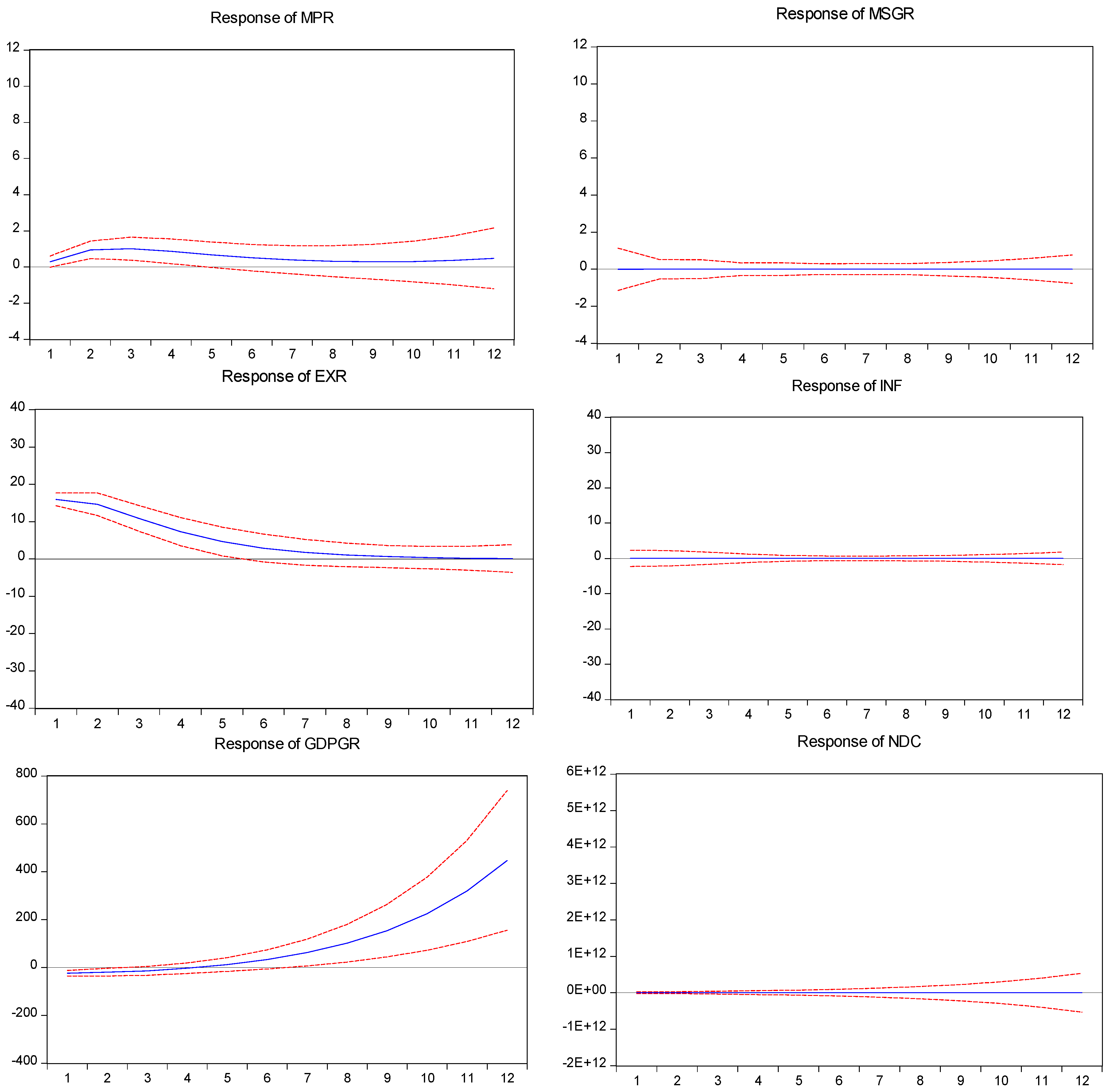
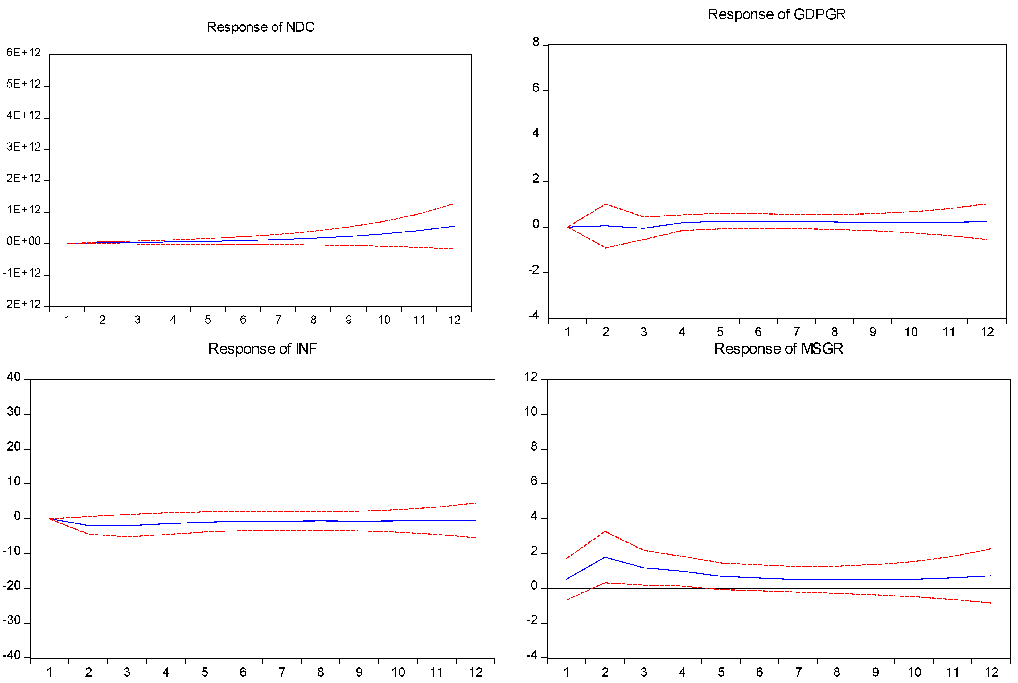
4.1. Impulse Response Analyses

In Figure 1 below, the thick blue lines are the IRFs while the red dotted lines are the one standard deviation confidence intervals. As depicted, the responses of the macroeconomic variables, namely, MPR, MSGR, EXR, INF, GDPGR and NDC, to shocks from oil price exhibited homogeneous effects throughout the period, both in magnitude and direction.

In Figure 1 is how a 1% dispersion in the price of oil was responded to by the variables. From the figure, clearly, oil price shocks did not attract any noticeable response, especially in the short run from, the variables. All through, their responses were very sluggish.

In Figure 2, the variables exr, rate, gdpgr and monetary policy rate responded noticeably to a 1% dispersion in the shock from the price of a commodity. A fall in monetary policy was noticed at the beginning of the period but this changed in the second and fourth periods such that a steady increase was recorded for the rest of the period. This resulted in a continuous fall in the exchange rate, suggesting appreciation of currency. In the fifth period, the GDP also rose significantly all through compared to its initial fall.

Three variables, namely, GDP growth rate, inflation and supply of money, exhibited a significant response to shocks in the monetary policy rate, as shown in Figure 3, below by responding noticeably to a 1% dispersion in the shock. The others remained inactive to shocks from the monetary policy rate.

It can be inferred from Figure 4 that monetary policy and supply of money responded noticeably (1%) to shocks from the exchange rate.

4.2. Forecast Error Variance Decompositions Analysis

Three major variables showed relevance here, namely, MPR, EXR and GDPGR, whereas the remaining ones had no influence.

Table 6. MPR variance decomposition.

Period	S.E.	OPV	CPV	NDC	GDPgr	INF	EXR	MSgr	MPR
3	4.475124	4.36 × 10−6	10.17958	5.66 × 10−5	0.335233	9.996381	17.43934	0.143394	61.90601
6	5.956191	3.23 × 10−6	9.319766	3.71 × 10−5	1.280981	9.764982	30.99097	1.827320	46.81594
9	7.026602	7.73 × 10−6	7.669539	2.68 × 10−5	1.856150	7.693765	31.86595	14.40582	36.50874
12	9.596733	3.81 × 10−5	4.337483	1.54 × 10−5	1.784839	4.611530	19.38965	49.99995	19.87649

below shows how shocks from each of the variables contributed to monetary policy rate movement. It can be inferred from the table that, except for itself, the growth rate in supply of money, inflationary rate, price of commodity and exchange rate were the greatest influencers of the movement of changes in monetary policy. For exchange rate, a 17.44% influence was recorded in the beginning of the period but appreciated to 31% during the third period, then dropping to 19.39% in the end. Similarly, at the start of the period, the rate in the growth of supply of money was 0.14% but ended up the period with an appreciable value of 50%, compared against the 10% and 4.61% recorded by inflation at the start and end of the period, respectively. Another movement was that of the price of a commodity that ended with 4.38% compared to the starting value of 10%.

Further analysis is contained in

Table 7. EXR variance decomposition.

Period	S.E.	OPV	CPV	NDC	GDPgr	INF	EXR	MSgr	MPR
3	166.1394	10.01 × 10−6	4.307193	0.000538	0.658041	0.985044	93.63537	0.013494	0.400321
6	275.6775	6.95 × 10−6	3.240690	0.000485	1.539355	3.140111	91.67701	0.013452	0.388893
9	430.5304	3.03 × 10−5	21.76515	0.000356	2.317943	4.858448	70.82463	0.012107	0.221338
12	816.8864	6.62 × 10−5	58.94114	0.000177	2.208229	3.414434	35.29079	0.024161	0.121004

, which shows how shocks from each of the variables contributed to the exchange rate movement. It can also be inferred from the table that, except itself, the price of a commodity exhibited the most influence by ending the period with 58.94% compared against the starting value of 4.31%. On the other hand, the marginal value of the influence of GDP ended the period with 2.21% compared to the starting value of 0.66%. Inflation started the period with 0.98% and recorded 3.41% towards the end.

Aside from shock to itself, it was monetary policy (encompassing interest rates) that influenced real GDP growth rate, as shown in

Table 8. Variance decomposition of GDPGR.

Period	S.E.	OPV	CPV	NDC	GDPGR	INF	EXR	MSGR	MPR
3	6.228362	4.93 × 10−6	0.000141	0.841456	96.49658	0.074595	0.014869	0.118110	2.454247
6	6.281070	4.88 × 10−6	0.000141	0.835408	94.90033	0.488358	0.435774	0.281881	3.058101
9	6.331746	4.92 × 10−6	0.000140	1.118283	93.44318	1.080032	0.799203	0.347002	3.212151
12	6.445082	6.75 × 10−6	0.000136	3.619285	90.28285	1.470141	1.109168	0.364309	3.154106

. In essence, the contributions of other variables to GDPgr shocks remained unnoticeable through the period under consideration.

In summary, we commenced our analysis with monetary policy rate (MPR) where four major shocks can be inferred apart from its own shock. The summary analyses of the impulse responses and forecast error-correction decompositions of the study show that shocks from commodity price affect the macroeconomic performance of the regional economy more than oil price shocks, as the impact of shocks from oil prices was very negligible throughout the study period. To start with, the study revealed that monetary policy rate, exchange rate and economic growth (measured as GDPgr) significantly responded to changes in the price of a commodity compared to the oil price, which has no effect. This suggests the existence of two major hypotheses within this region: the overshooting hypothesis and the J-Curve hypothesis. Responsible for this could be predominantly the nature of the countries within the EAC in that they are a raw agricultural exporting region whose products are susceptible to foreign dictates. An upward movement of commodity price can boost the GDP of the region [11]. Furthermore, shocks from the monetary policy rate had great influence on the inflationary and money supply rates, as revealed by the impulse response and variance decomposition outcomes. This is another confirmation about the relationship between money supply, inflation and monetary policy (lending rate). Theoretically, any action by a monetary authority is usually targeted at controlling the supply of money and inflation rate [75]. In addition, the behaviours of economic growth rate, money supply and monetary policy rate are mostly dictated by the exchange rate. This finding is in tandem with [57]. In dealing with this kind of scenario, [5] suggests a hybrid contractionary monetary policy during the period of boom and an expansionary policy in the time of burst [76], which are recommended for the countries of the region. Finally, the transmission effects of shocks from the price of a commodity viz-a-viz the exchange rate to GDPgr through the lending rate (monetary policy rate) and supply of money constitute the major means of linkage within the EAC region. In other words, the dynamism in monetary policy was caused by shocks from the price of a commodity, which subsequently affected GDP via the exchange rate in the EAC.

5. Conclusions

In order to accomplish the study’s set aims, we formulated the Structural-VAR model. The technique helped to comprehend how the dynamics in monetary policy interacts with other macroeconomic variables in the EAC sub-region of Africa. The main conclusion from our analysis is that commodity price shocks (oil and non-oil) significantly affect the exchange rate and that adjustments in monetary policy (interest rate and money supply) in turn are instrumental in transmitting this exchange rate effect to economic growth. This shows how vulnerable the EAC countries are to strong and persistent variations in world commodity prices. This paper further contributes to the literature that describes the vulnerability of many African countries with open economies to large changes in the terms of trade caused by the variable import price of oil (quoted in US dollar) and the market-given export price of their agricultural products.

It is therefore suggested that the current fall in prices of commodities, as evident in the impulse response outcome, should be a clarion call to member countries to rejig their economic policies on economic diversification of the member states’ economy. It should serve as a reminder to policy makers on how vulnerable their economies are subject to volatility in commodity price variations. The need to diversify the productive and export base of member countries compared to the continuous dependence on one or a few products as major source of income is hereby advocated. Further, there is the need for private–public partnership for the promotion of regional cooperation among member countries. Finally, the results provide a template for the EAC in making decisions regarding a currency union, whether to adopt a free-floating external exchange rate (which allows the EAC’s common monetary policy to focus on local needs), a managed external exchange rate (with less EAC monetary policy autonomy and some exchange rate flexibility relative to main external trade partners), or a fixed parity relative to the US dollar or the euro or a currency basket as the nominal anchor (which gives up EAC monetary policy sovereignty but could avoid major exchange rate shocks against the main external trade partners). This EAC decision is vital for the sustainability of the future common currency.

References

1. East Africa Economic Outlook. Macroeconomic Development and Prospects-Political Economy of Regional Integration; African Development Bank Group: Abidjan, Cote d’Ivoire, 2019. [Google Scholar]
2. Dillon, B.M.; Barrett, C. Global Oil Prices and Local Food Prices: Evidence from East Africa. Am. J. Agric. Econ. 2015, 98, 154–171. [Google Scholar] [CrossRef]
3. Ng’ang’a, W.I.; Chevallier, J.; Ndiritu, S. Investigating Fiscal and Monetary Policies Coordination and Public Debt in Kenya: Evidence from Regime-Switching and Self-Exciting Threshold Autoregressive Models; halshs-02156495; Kiel Institute for the World Economy (IfW Kiel): Kiel, Germany, 2019. [Google Scholar]
4. Addison, T.; Ghoshray, A.; Stamatogiannis, M.P. Agricultural Commodity Price Shocks and Their Effect on Growth in Sub-Saharan Africa. J. Agric. Econ. 2015, 67, 47–61. [Google Scholar] [CrossRef] [Green Version]
5. Chuku, C.; Simpasa, A.; Oduor, J. Macroeconomic Consequences of Commodity Price Fluctuations in African Economies. Afr. Dev. Rev. 2018, 30, 329–345. [Google Scholar] [CrossRef]
6. Chileshe, P.M.; Chisha, K.; Ngulube, M. The effect of external shocks on macroeconomic performance and monetary. Int. J. Sustain. Econ. 2018, 10, 18–40. [Google Scholar]
7. Cieślik, E. International Trade in East Africa: The Case of the Intergovernmental Authority on Development. J. Pan Afr. Stud. 2015, 8, 79–96. [Google Scholar]
8. Afesorgbor, S.K. Regional Integration, Bilateral Diplomacy and African Trade: Evidence from the Gravity Model. Afr. Dev. Rev. 2019, 31, 492–505. [Google Scholar] [CrossRef]
9. Umulisa, Y. Estimation of the East African Community’s trade benefits from promoting intra-regional trade. Afr. Dev. Rev. 2020, 32, 55–66. [Google Scholar] [CrossRef]
10. Christensen, B.V. Challenges of Low Commodity Prices for Africa; Bank of International Settlement Papers No 87; Bank of International Settlement: Basel, Switzerland, 2016. [Google Scholar]
11. African Development Bank Group. African Economic Outlook; African Development Bank Group: Abidjan, Côte d’Ivoire, 2018. [Google Scholar]
12. Omolade, A.; Ngalawa, H.; Kutu, A. Crude oil price shocks and macroeconomic performance in Africa’s oil-producing countries. Cogent Econ. Financ. 2019, 7, 1607431. [Google Scholar] [CrossRef]
13. Alenoghena, R.O. Oil Price Shocks and Macroeconomic Performance of the Nigerian Economy: A Structural VAR Approach. Facta Univ. Ser. Econ. Organ. 2020, 17, 299–316. [Google Scholar] [CrossRef]
14. Bynoe, A.J. Monetary and Fiscal Influences on Economic Activities in African Countries; African Review of Money Finance and Banking, No. 1/2; Giordano Dell-Amore Foundation, 1994; pp. 97–107. Available online: http://www.jstor.org/stable/23027487 (accessed on 8 November 2021).
15. Alavi, S.E.; Moshiri, S.; Sattarifar, M. An Analysis of the Efficiency of the Monetary and Fiscal Policies in Iran Economy Using IS–MP–AS Model. Procedia Econ. Financ. 2016, 36, 522–531. [Google Scholar] [CrossRef] [Green Version]
16. Cavalcanti, M.A.; Vereda, L.; Doctors, R.D.B.; Lima, F.; Maynard, L. The macroeconomic effects of monetary policy shocks under fiscal rules constrained by public debt sustainability. Econ. Model. 2018, 71, 184–201. [Google Scholar] [CrossRef]
17. Ismail, S.F.; Sek, S.K. Investigating the effects of fiscal and monetary policy on economic performance: Dynamic panel threshold regression analysis. In Proceedings of the AIP Conference, Penang, Malaysia, 10–12 December 2018; Volume 2184. [Google Scholar] [CrossRef]
18. Büyükbaşaran, T.; Çebi, C.; Yılmaz, E. Interaction of monetary and fiscal policies in Turkey. Cent. Bank Rev. 2020, 20, 193–203. [Google Scholar] [CrossRef]
19. Le, H.V.; Pfau, W.D. VAR Analysis of the Monetary Transmission Mechanism in Vietnam. Appl. Econom. Int. Dev. 2009, 9, 165–179. [Google Scholar]
20. Can, U.; Bocuoglu, M.E.; Can, Z.G. How does the monetary transmission mechanism work? Evidence from Turkey. Borsa Istanb. Rev. 2020, 20, 375–382. [Google Scholar] [CrossRef]
21. Nkalu, C.N. Empirical Analysis of Demand for Real Money Balances in Africa: Panel Evidence from Nigeria and Ghana. Afr. Asian Stud. 2020, 19, 363–376. [Google Scholar] [CrossRef]
22. Arwatchanakarn, P. Monetary Policy Shocks and Macroeconomic Variables: Evidence from Thailand. In Computational Intelligence; ResearchGate, 2019; Available online: https://doi.org/10.1007/978-3-030-04263-9_16 (accessed on 5 March 2020).
23. Ndubuisi, G.O. Interest Rate Channel of Monetary Policy Transmission Mechanisms: What Do We Know about It? 2015. Available online: https://doi.org/10.2139/ssrn.2623036 (accessed on 5 March 2021).
24. Amusa, H.; Fadiran, D. The J-Curve Hypothesis: Evidence from Commodity Trade Between South Africa and the United States. Stud. Econ. Econ. 2019, 43, 39–62. [Google Scholar] [CrossRef]
25. Mishkin, F.S. Symposium on the Monetary Transmission Mechanism. J. Econ. Perspect. 1995, 9, 3–10. [Google Scholar] [CrossRef] [Green Version]
26. Njimanted, F.G.; Daniel Akume, D.; Mukete, E.M. The Impact of Key Monetary Variables on the Economic Growth of the CEMAC Zone. Expert J. Econ. 2016, 4, 54–67. [Google Scholar]
27. Olamide, E.G.; Maredza, A. Regional Effects of Monetary Policy on Economic Growth of ECOWAS: An S-VAR Approach. J. Dev. Areas 2019, 53, 205–223. [Google Scholar] [CrossRef]
28. Antwi, S.; Issah, M.; Patience, A.; Antwi, S. The effect of macroeconomic variables on exchange rate: Evidence from Ghana. Cogent Econ. Financ. 2020, 8, 1821483. [Google Scholar] [CrossRef]
29. Hassan, A.S.; Meyer, D.F. Analysis of the Non-Linear Effect of Petrol Price Changes on Inflation in South Africa. Int. J. Soc. Sci. Hum. Stud. 2020, 12, 34–49. [Google Scholar]
30. Schmitt-Grohé, S.; Uribe, M. How important are terms-of-trade shocks? Int. Econ. Rev. 2018, 59, 85–111. [Google Scholar] [CrossRef] [Green Version]
31. Drechsel, T.; Tenreyro, S. Commodity booms and busts in emerging economies. J. Int. Econ. 2018, 112, 200–218. [Google Scholar] [CrossRef]
32. Roch, F. The adjustment to commodity price shocks. J. Appl. Econ. 2019, 22, 437–467. [Google Scholar] [CrossRef]
33. Gabriel, L.F.; Ribeiro, L.C.D.S. Economic growth and manufacturing: An analysis using Panel VAR and intersectoral linkages. Struct. Chang. Econ. Dyn. 2019, 49, 43–61. [Google Scholar] [CrossRef]
34. Ezeaku, H.C.; Ibe, I.G.; Ugwuanyi, U.B.; Modebe, N.J.; Agbaeze, E.K. Monetary Policy Transmission and Industrial Sector Growth: Empirical Evidence from Nigeria. Sage Open 2018, 8, 2158244018769369. [Google Scholar] [CrossRef]
35. Hoang, T.T.; Thi, V.A.N. The impact of macroeconomic factors on the inflation in Vietnam. Manag. Sci. Lett. 2020, 10, 333–342. [Google Scholar] [CrossRef]
36. Ciora, Z. Monetary Policy, Inflation and the Causal Relation between the Inflation Rate and Some of the Macroeconomic Variables. Procedia Econ. Financ. 2014, 16, 391–401. [Google Scholar] [CrossRef] [Green Version]
37. Hatmanu, M.; Cautisanu, C.; Ifrim, M. The Impact of Interest Rate, Exchange Rate and European Business Climate on Economic Growth in Romania: An ARDL Approach with Structural Breaks. Sustainability 2020, 12, 2798. [Google Scholar] [CrossRef] [Green Version]
38. Iddrisu, S.; Harvey, S.K.; Amidu, M. The Impact of Monetary Policy on Stock Market Performance: Evidence from Twelve African Countries. Res. Int. Bus. Financ. 2017, 42, 1372–1382. [Google Scholar] [CrossRef]
39. Akosah, N.K.; Alagidede, I.P.; Schaling, E. Testing for asymmetry in monetary policy rule for small-open developing economies: Multiscale Bayesian quantile evidence from Ghana. J. Econ. Asymmetries 2020, 22, e00182. [Google Scholar] [CrossRef]
40. Asongu, S. New empirics of monetary policy dynamics: Evidence from the CFA franc zones. Afr. J. Econ. Manag. Stud. 2016, 7, 164–204. [Google Scholar] [CrossRef] [Green Version]
41. Famoroti, J.O.; Tipoy, C.K. Macroeconomic Effects of External Monetary Policy Shocks to Economic Growth in West Africa; Stellenbosch University: Cape Town, Western Cape, South Africa, 2019; Available online: https://www.ekon.sun.ac.za/phdconference2019/famoroti-o.-jonathan.pdf (accessed on 5 March 2020).
42. Omojolaibi, J.A.; Egwaikhide, F.O. A Panel Analysis of Oil Price Dynamics Fiscal Stance and Macroeconomic Effects: The Case of Some Selected African Countries. Cent. Bank Niger. Econ. Financ. Rev. 2013, 51, 61–91. [Google Scholar]
43. Etornam, D.K. The Impact of Oil Price Shocks on the Macroeconomy of Ghana. J. Poverty Investig. Dev. 2015, 9, 37–54. [Google Scholar]
44. Chiweza, J.T.; Aye, G.C. The effects of oil price uncertainty on economic activities in South Africa. Gen. Appl. Econ. 2018, 6, 1518117. [Google Scholar] [CrossRef] [Green Version]
45. Odhiambo, S.A. Money, Inflation and Output: Understanding the cornerstones of a monetary union in East Africa Community. Eur. Sci. J. 2017, 13, 503–520. [Google Scholar] [CrossRef]
46. Buigut, S. Monetary Policy Transmission Mechanism: Implications for the Proposed East African Community (EAC) Monetary Union. 2009. Available online: http://www.csae.ox.ac.uk/conferences/2009-EdiA/paperlist.html (accessed on 10 September 2021).
47. Abuka, C.; Alinda, R.K.; Minoiu, C.; Peydró, J.-L.; Presbitero, A.F. Monetary policy and bank lending in developing countries: Loan applications, rates, and real effects. J. Dev. Econ. 2019, 139, 185–202. [Google Scholar] [CrossRef]
48. Nyorekwa, E.T.; Nicholas, M.; Odhiambo, N.M. Monetary policy and economic growth dynamics in Uganda. Banks Bank Syst. 2014, 9, 18–28. [Google Scholar]
49. Kamaan, C.K. Effect of Economic Growth in Kenya. Int. J. Bus. Commer. 2014, 3, 11–24. Available online: www.ijbcnet.com (accessed on 5 March 2020).
50. Ayubu, V.S. Monetary Policy and Inflation Dynamics: An Empirical Case Study of Tanzania Economy. Unpublished Master’s Thesis in Economics, Umea, Sweden. 2013. [Google Scholar]
51. Wetite, T.B. The Relative Effectiveness of Monetary and Fiscal Policies on Industrial Growth of Ethiopia. 2021, Volume 8. Available online: www.ijrar.org (accessed on 10 September 2021).
52. Beyene, S.D.; Kotosc, B. Is Fiscal or Monetary Policy More Effective on Economic Growth? an Empirical Evidence in The Case of Ethiopia. J. Afr. Res. Bus.Technol. 2020, 2020, 124855. [Google Scholar] [CrossRef]
53. Davoodi, H.; Dixit, S.; Pinter, G. Monetary Transmission Mechanism in the East African Community: An Empirical Investigation; IMF Working paper; International Monetary Fund: Washington, DC, USA, 2013; Volume 2013, No. 39. [Google Scholar]
54. Berg, A.; Charry, L.; Portillo, R.; Vlcek, J. The Monetary Transmission Mechanism in the Tropics: A Narrative Approach; IMF Working Paper; IMF: Washington, DC, USA, 2013; p. 197. [Google Scholar]
55. Twinoburyo, E.N.; Odhiambo, N.M. Monetary Policy and Economic Growth in Kenya: The Role of Money Supply and Interest Rates. UNISA Economic Research Working Paper Series 11/2016. 2016. Available online: http://hdl.handle.net/10500/20712 (accessed on 5 March 2020).
56. Caporale, G.M.; Gil-Alana, L. Prospects for a Monetary Union in the East Africa Community: Some Empirical Evidence. S. Afr. J. Econ. 2020, 88, 174–185. [Google Scholar] [CrossRef] [Green Version]
57. Omolade, A.; Ngalawa, H. Monetary policy transmission mechanism and growth of the manufacturing sectors in Libya and Nigeria: Does exchange rate regime matter? J. Entrep. Bus. Econ. 2017, 5, 67–107. [Google Scholar]
58. Olamide, E.G.; Maredza, A. A dynamic regression panel approach to the determinants of monetary policy and economic growth: The SADC experience. Afr. J. Econ. Manag. Stud. 2019, 10, 385–399. [Google Scholar] [CrossRef]
59. Olamide, E.G.; Maredza, A. The Short and Long Run Dynamics of Monetary Policy, Oil Price Volatility and Economic Growth in the CEMAC Region. Asian Econ. Financ. Rev. 2021, 11, 78–89. [Google Scholar] [CrossRef]
60. Chudik, A.; Pesaran, M.H. Large Panel Data Models with Cross-Sectional Dependence. A Survey, Federal Reserve Bank of Dallas Globalisation and Monetary Policy Institute Working Paper. 2013, p. 153. Available online: http://www.dallasfed.org/assets/documents/institute/wpapers/2013/0153.pdf (accessed on 10 September 2021).
61. Pesaran, M.H.; Im, K.S.; Shin, Y. Testing for unit roots in heterogeneous panels. J. Econom. 2003, 115, 53–74. [Google Scholar] [CrossRef]
62. Moon, H.R.; Perron, B. Testing for a Unit Root in Panels with Dynamic Factors. J. Econom. 2004, 122, 81–126. [Google Scholar] [CrossRef] [Green Version]
63. Bai, J.; Ng, S. A PANIC Attack on Unit Roots and Cointegration. Econometrica 2004, 72, 1127–1177. [Google Scholar] [CrossRef] [Green Version]
64. Breitung, I.; Das, S. Testing for Unit Root in Panels with a Factor Structure. Econom. Theory 2008, 24, 88–108. [Google Scholar] [CrossRef]
65. Svensson, E. Regional Effects of Monetary Policy in Sweden; Working Paper 9; Department of Economics, School of Economics and Management, Lund University: Lund, Sweden, 2013. [Google Scholar]
66. Dritsakis, N. Demand for Money in Hungary: An ARDL Approach. Rev. Econ. Financ. 2011, 1, 1–16. [Google Scholar]
67. Trade Performance and Commodity Dependence, Economic Development in Africa. In Proceedings of the United Nations Conference on Trade and Development, Geneva, Switzerland, 26 February 2004.
68. McMillin, W.D. The Effects of Monetary Policy Shocks: Comparing Contemporaneous versus Long-Run Identifying Restrictions. South. Econ. J. 2001, 67, 618–636. [Google Scholar]
69. Paramanik, R.N.; Kamaiah, B. A Structural Vector Autoregression Model for Monetary Policy Analysis in India. Margin—J. Appl. Econ. Res. 2014, 8, 401–429. [Google Scholar] [CrossRef]
70. Rotimi, M.E.; Ngalawa, H. Oil Price Shocks and Economic Performance in Africa’s Oil Exporting Countries. Acta Univ. Danub. 2017, 13, 169–188. [Google Scholar]
71. Arias, J.E.; Rubio-Ramirez, J.F.; Waggoner, D.F. Inference Based on SVARs Identified with Sign and Zero Restrictions: Theory and Applications. Econometrica 2018, 86, 685–720. [Google Scholar] [CrossRef]
72. Elbourne, A. The UK housing market and the monetary policy transmission mechanism: An SVAR approach. J. Hous. Econ. 2008, 17, 65–87. [Google Scholar] [CrossRef]
73. Demachi, K. The Effect of Crude Oil Price Change and Volatility on Nigerian Economy; MPRA Paper 41413; Munich Personal RePEc Archive-MPRA; University Library of Munich: Munich, Germany, 2012. [Google Scholar]
74. Tevdovski, D.; Petrevski, G.; Bogoev, J. The effects of macroeconomic policies under fixed exchange rates: A Bayesian VAR analysis. Econ. Res -Ekon. Istraživanja 2019, 32, 2138–2160. [Google Scholar] [CrossRef] [Green Version]
75. Phetole, S.; Ogujiuba, K. Is there a Nexus between Inflation, Exchange Rate and Unemployment in South Africa: An Econometric Analysis. Montenegrin J. Econ. 2021, 17, 45–58. [Google Scholar]
76. Ogujiuba, K.; Mbangata, T. A Comparative Analysis of Macroeconomic Outcomes amongst the BRICS Countries (2000–2015). J. Int. Econ. 2020, 11, 49–63. [Google Scholar]
Figure 1. Response to oil price shock in EAC.
Sustainability 14 03490 g001
Figure 2. Response to shocks from the price of a commodity.
Sustainability 14 03490 g002
Figure 3. Response to shocks from the monetary policy rate.
Sustainability 14 03490 g003
Figure 4. Response to the exchange rate shock.
Sustainability 14 03490 g004aSustainability 14 03490 g004b