Optimization Model for Sustainable End-of-Life Vehicle Processing and Recycling

Abstract

The aim of this paper is to provide a mathematical programming model for sustainable end-of-life vehicle processing and recycling. Environmental benefits and resource efficiency are achieved through the incorporation of a processing and recycling network that is based on industrial symbiosis whereby waste materials are converted into positive environmental externalities aimed at decreasing pollution and reducing the need for raw materials. A mixed-integer programming model for optimizing the exchange of material flows in the network is developed and applied on a real case study. The model selects the components that maximize reusable/recyclable material output while minimizing network costs. In addition, GHG emissions are calculated to assess the environmental benefits of the network. The model finds the optimal processing routes while maximizing the yield of the components of interest, maximizing profit, minimizing cost, or minimizing waste depending on which goals are chosen. The results are analyzed to provide insights about the network and the utility of the proposed methodology to improve sustainability of end-of-life vehicle recycling.

1. Introduction

Sustainable management of End-of-Life Vehicles (ELVs) has become a global priority due to the environmental concerns. One of the United Nations’ sustainable development goals is to ensure sustainable consumption and production patterns (Goal 12) [1]. Reducing waste generation through prevention, reduction, recycling, and reuse is one priority in Goal 12. As defined by the European Directive of ELVs 2000/53/EC, End-of-Life Vehicles are “vehicles that have become waste”, and waste is defined as “any substance or object which the holder discards, or intends to discard, or is required to discard” [2]. It was estimated that by the end of 2020, the global number of ELVs will exceed 100 million [3]. Recycling ELVs saves energy and natural resources. According to Steel Recycling Institute, “recycling one ton of steel conserves 2500 pounds of iron ore, 1400 pounds of coal, and 120 pounds of limestone” [4]. This resulted in an energy saving from steel recycling that is equivalent to powering 20 million homes for the year 2012 [5]. The recycling process has been adopted by many countries worldwide [6,7,8,9,10,11,12,13,14,15,16,17,18,19,20,21,22,23,24,25,26]. There are many successful experiences in recycling ELVs worldwide, including in Europe, United States, Russia, Netherlands, New Zealand, China, Japan, Canada, Australia, Turkey, South Korea, and others [2,3,4,5,6,7,9,14,27]. A recent paper provided a comprehensive review of the ELVs literature by presenting 232 peer-reviewed articles from the period of 2000–2019 [6]. The article highlighted the major gaps in the literature, which include the lack of comprehensive ELV network-design models and methodologies that incorporate nodes beyond the shredding stage and the beneficial synergism with existing related companies.

Research areas related to End-of-Life Vehicles are diverse. While some papers present the ELVs management process worldwide [10,11,12,13,14,15,16,17,18], others apply mathematical modeling to solve ELVs from different perspectives [9,14,19,20,21,22,27,28,29,30].

Reverse logistics as defined by [31] is “the process of planning, implementing, and controlling the efficient, cost effective flow of raw materials, in-process inventory, finished goods and related information from the point of consumption to the point of origin for the purpose of recapturing value or proper disposal” [31]. In the literature, extensive studies are available on recycling products using a reverse-logistics concept [32,33,34,35]. Furthermore, more than 76% of the studies dealt with the open-loop supply chain whereby the material suppliers, production facilities, and distribution services are only linked in a feed forward flow manner; hence, the closed-loop supply chain that includes reverse logistics to collect and process used products was not studied [36].

In the early 1996, an initiative by Recourse Recycling Systems, Inc. (RRSI) collaborating with Vehicle Recycling Partnership (VRP) began to document the challenges for ELVs recycling [27]. After years of research, the initiative resulted in another project: Auto Recycling Documentation Project (ARD). The ARD project aimed to find “methods of collection and vehicle disassembly that optimize the net value of post-consumer vehicles in terms of recyclable material recovery in addition to conventional recovery of reusable parts” [27]. The findings from the project identified some methods and costs of recovering ELVs’ non-metal materials (glass, foam, plastics, textiles, and elastomers).

The aim of the research in this paper is to present a mathematical programming model to solve the end-of-life vehicle problem utilizing the concept of industrial symbiosis. The model takes into account full interactions between several entities. The proposed model consisting of mixed-integer programming, superstructure optimization, and data blocks feeding these structures aims to encourage circular economy and industrial symbiosis in the network. By finding the optimal processing routes that maximize the flow exchange, profit is maximized, while costs and expenses are minimized. In addition, the amounts of CO₂ emissions in the network are reduced by applying the Eco-Industrial Park approach.

The remainder of this paper is organized as follows: Section 2 proposes the network superstructure and provides a mathematical programming model for the optimal network design. Section 3 presents a case study of ELVs in Qatar. Finally, Section 4 outlines the conclusions.

2. Proposed Network Superstructure

The developed network is shown in Figure 1 and shows the interconnections between the different processing entities. These entities include power plants, dismantling facilities, waste-to-energy plants, wastewater-treatment plants, plastic companies, aluminum companies, steel companies, glass companies, tire-recycling companies, and battery-recycling companies. The anchor entity that generates the most waste/byproducts is the dismantling facility [13,20,30]. The dismantling facility is the core of the network, as it sends out scrap materials of different types to the corresponding industries.

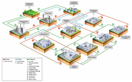
Figure 1. Proposed network for End-of-Life Vehicles processing and recycling; Copyrighted by the authors, Registration Number VAu001381819.

The network is based on material flows exchange from one entity to the other. Figure 1 is illustrated in a geo-spatial format; however, the entities form a network without any location restriction. As presented by [20], material exchanges have five types: type A is waste exchanges through third party; type B is within facility, firm, or organization; type C is between firms collocated in a defined Eco-Industrial Park; type D is between local firms that are not collocated; and type E is between virtually organized firms across a broader region [13,20]. The main types for flows to build an EIP are types C–E [30]. In the proposed network, the material exchanges through different ways of transportation; trucks and pipelines are the main methods. The modeled network is shown in Figure 2. The figure shows the processing pathways going from the collection points (CP₁, CP2, …, CP_I) to the dismantling and shredding facilities (DF₁, DF₂, …, DF_J). This is followed by the different processing facilities, such as tire and battery further processing, and finally, the introduction of useful products to market. More details about the different components and nodes of the overall superstructure used in the development of the model are given in Appendix A.

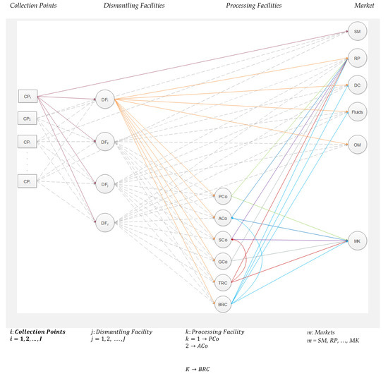
Figure 2. Proposed Network: burgundy, ELVs flow; orange, parts flow; green, plastics flow; dark blue, aluminum flow; purple, steel flow; solid gray, glass flow; red, tire flow; blue, battery flow; dashed gray, future interactions/flows.

2.1. Optimization Model

The present section shows the main features of the proposed optimization model for designing the End-of-Life Vehicles (ELVs) network.

2.1.1. Problem Statement

The proposed optimization approach seeks to minimize both fixed and variable costs associated with the Eco-Industrial Park for End-of-Life Vehicles. The mathematical model consists of four sets of nodes designed to operate as a network: collection points (i), dismantling facilities (j), processing facilities (k), and markets (m). Firstly, vehicles that have become waste are sent to collection points (i) where they are stockpiled for further processing. Secondly, vehicles are sent to secondhand markets (sh ∈ m) and/or dismantling facilities (j) where they are sold as secondhand vehicles and/or dismantled into main pieces and materials, respectively. Thirdly, vehicles’ pieces and materials are sent to markets (m) and/or processing facilities (k). Fourthly, final products from processing facilities (k) are sent to markets (m), whereas specific intermediate products are exchanged among facilities for further processing. The optimization procedure selects the most suitable combination of network components. Therefore, an integrated relationship among nodes was considered in the present analysis. The EIP design must meet operating constraints.

2.1.2. Problem Representation

A source-sink structure representation was employed to embed potential Eco-Industrial Park for End-of-Life Vehicles (ELV) designs of interest. The indices g and g′ denote analogous main sets representing the source-and-sink nodes structure of the network, respectively. Accordingly, the main set of network nodes/components g and g′ are given as follows:

$$g=\left\{i, j,k,m\right\}{g}^{\prime }=\left\{j,k,m\right\}$$

where i denotes the collection points, j the dismantling facilities, k the processing facilities, and m the markets. The index $k=\left\{PCo, ACo,SCo,GCo, TRC, BRC\right\}$ includes plastic company (PCo), aluminum company (ACo), steel company (SCo), glass company (GCo), tire-recycling company (TRC), and battery-recycling company (BARC). The index $m=\left\{sh, rp,dc,fl, ot, mk\right\}$ comprises secondhand market (sh), reusable parts market (rp), disposal center (dc), fluids market (fl), other materials market (ot), and commercialization markets (mk).

Similarly, the index $h=\left\{pl,al,st,gl, tr, bt, vf, om, nr\right\}$ defines the type of material/part found in a vehicle. The symbol pl symbolizes plastic, al aluminum, st steel, gl glass, tr tire, bt battery, vf vehicle fluids, om other materials, and nr non-recyclable materials. The index $t\in tr=\left\{ru, fi,st\right\}$ includes ru rubber, fi fiber, and st steel. Additionally, the index $b\in bt=\left\{bf,pb, hz, pl\right\}$ includes bf battery fluid, pb lead, hz hazardous materials, and pl plastic. Likewise, the index $f\in vf=\left\{to,co,eo,ga, cf, bf\right\}$ comprises to transmission oil, co coolant, eo engine oil, ga gasoline, cf cfc-hfc, and bf battery fluid. The index $o\in om=\left\{cu,pb, pt\right\}$ contains cu copper, pt platinum, and pt lead. Similarly, the index $n\in nr=\left\{dis, hz\right\}$ includes dis (disposable materials) and hz (hazardous materials).

2.2. Model Formulation

The mass and energy balances for the End-of-Life Vehicles’ nodes/stages are presented next. Variables are denoted in italic font, while parameters are represented by regular font. These balances represent the equality constraints in the model. Inequality constraints representing amounts of raw materials and capacity constraints will be dealt with later.

2.2.1. Model Constraints

Collection Points (i)

The collection points are used to stockpile vehicles that have become waste. Accordingly, the number of vehicle type v stocked at collection points can be estimated as follows:

$${\mathrm{NV}}_v={\sum }_i C{P}_{v,i} ,\forall v$$

(1)

where NV_v is a parameter denoting the total number of vehicles type v sent to all collection points, and CP_v,i is the number of vehicles v sent to collection point i. The index $v=\left\{ge, de\right\}$ includes ge gasoline engine vehicles and de diesel engine vehicles. Moreover, from collection points, a number of vehicles can be sent to a secondhand vehicle market (SH_v,i,m) as follows:

$$S{H}_{v,i,m}={\mathrm{SHP}}_{v,i,m} \left(C{P}_{v,i}\right), \forall v,i, m=sh$$

(2)

where SHP_v,i,m is a parameter denoting the share of vehicles v sent from collection point i to mth market. The general mas balance in the collection points node is given as follows:

$$C{P}_{v,i}={\sum }_j D{F}_{v,i,j}+{\sum }_{m\in sh} S{H}_{v,i,m}, \forall v,i$$

(3)

where DF_v,i,j is the number of vehicles v sent from the ith collection point to the jth dismantling facility.

Dismantling Facilities (j)

The yield of materials at the dismantling facilities can be given as follows:

$$MATERIA{L}_{v,h,j}={\mathrm{YIELDP}}_{v,h }\left({\sum }_{i}D{F}_{v,i,j}\right), \forall v,h,j$$

(4)

where MATERIAL_v,h,j is the yield of material h from vth vehicle at dismantling facility j, and YIELDP_v,h is a parameter denoting the yield of material h from the vth vehicle.

The amount of material out of dismantling facilities to processing facilities is as follows:

$$P{F}_{v,h,j,k}={\mathrm{PFP}}_{v,h,k} \left(MATERIA{L}_{v,h,j}\right),h\in \left\{pl,al,st,gl,tr,bt\right\}; \forall v,j,k$$

(5)

where PF_v,h,j,k is the vehicle’s v type of material h sent from jth dismantling facility to kth processing facility, and PFP_v,h,k is a parameter indicating the type of material h from vehicle v sent to processing facility k.

The amount of material out of dismantling facilities to a reusable parts market is as follows:

$$R{P}_{v,h,j,m}={\mathrm{RPP}}_{v,h,m} \left(MATERIA{L}_{v,h,j}\right), h\in \left\{pl,al,st,gl,tr,bt\right\}; m=rp; \forall v,j$$

(6)

where RP_v,h,j,m is the vehicle’s v type of material h sent from jth dismantling facility to mth market, and RPP_v,h,m is a parameter indicating the share of type of material h from vehicle v sent to mth market.

The amount of material out of dismantling facilities that cannot be recovered/recycled must be sent to the disposal center as follows:

$$D{C}_{v,h,j,m}={\mathrm{DCP}}_{v,h,m} \left(MATERIA{L}_{v,h,j}\right), m=dc; \forall v,h,j$$

(7)

where DC_v,h,j,m is the vehicle’s v type of material h that cannot be recovered/recycled and must be disposed from the jth dismantling facility into mth market, and DCP_v,h,m is a parameter indicating the share of type of material h from vehicle v sent to mth market.

The amount of material out of dismantling facilities sent to fluids market is as follows:

$$F{L}_{v,f,j,m}={\mathrm{FLP}}_{v,f,m} \left({\sum }_{h\in vf}MATERIA{L}_{v,h,j}\right), m=fl; \forall v,f,j$$

(8)

where FL_v,f,j,m is the vth vehicle’s material f sent from jth dismantling facility to mth market, and FLP_v,f,m is a parameter indicating the share of material f from vehicle v sent to mth market.

The amount of material out of dismantling facilities sent to the other materials market is as follows:

$$O{M}_{v,o,j,m}={\mathrm{OMPP}}_{v,o,m} \left({\sum }_{h\in om}MATERIA{L}_{v,h,j}\right), m=ot; \forall v,o,j$$

(9)

where OM_v,o,j,m is the vth vehicle’s material o sent from jth dismantling facility to mth market, and OMPP_v,o,m is a parameter indicating the share of material o from vehicle v sent to mth market.

Tire-Recycling Company (TRC)

The amount of material out of the tire-recycling company sent to reusable parts market is given as follows:

$$T{R}_{v,g}={\mathrm{TRP}}_g \left({\sum }_h{\sum }_j{\sum }_{k\in TRC}P{F}_{v,h,j,k}\right) , g=m\left(rp\right); \forall v$$

(10)

where TR_v,g is the vth vehicle’s tires sent to gth node, and TRP_g is a parameter indicating the share of tires sent to gth node.

The amount of material out of the tire-recycling company sent to the steel company and commercialization markets is given as follows:

$$TR{C}_{v,t,g}=\left(1-{\sum }_{g\in m\left(rp\right)}{\mathrm{TRP}}_g\right){ \mathrm{TRCP}}_{t,g} \left({\sum }_h{\sum }_j{\sum }_{k\in TRC}P{F}_{v,h,j,k}\right), g\in \left\{k\left(SCo\right), m\left(mk\right)\right\}; \forall v,t$$

(11)

where TRC_v,t,g is the vth vehicle’s material t sent to gth node, and TRCP_t,g is a parameter indicating the percentage of material t sent to gth node.

Battery-Recycling Company (BARC)

The amount of material out of the battery-recycling company sent to reusable parts market is given as follows:

$$B{R}_{v,g}={\mathrm{BRP}}_g \left({\sum }_h{\sum }_j{\sum }_{k\in BRC}P{F}_{v,h,j,k}\right), g=m\left(rp\right) ; \forall v$$

(12)

where BR_v,g is the vth vehicle’s battery sent to gth node, and BRP_g is a parameter indicating the share of batteries sent to gth node.

The amount of material out of the battery-recycling company sent to the plastic company, disposal center, fluids market, and commercialization markets is given as follows:

$$BR{C}_{v,b,g}=\left(1-{\sum }_{g\in m\left(rp\right)}{\mathrm{BRP}}_g\right){ \mathrm{BRCP}}_{b,g} \left({\sum }_h{\sum }_j{\sum }_{k\in BRC}P{F}_{v,h,j,k}\right), g\in \left\{k\left(PCo\right),m\left(dc\right),m\left(fl\right), m\left(mk\right)\right\}; \forall v,b$$

(13)

where BRC_v,b,g is the vth vehicle’s material b sent to gth node, and BRCP_b,g is a parameter indicating the percentage of material b sent to gth node.

The capacity constraint associated with each component of the proposed end-of-life vehicle network are described as follows:

$$B_g {\mathrm{Cap}}_{h,g}^{\mathrm{Min}}\le M{F}_{h,g}\le B_g{ \mathrm{Cap}}_{h,g}^{\mathrm{Max}} , \forall h,g$$

(14)

where MF_h,g is a variable denoting the mass flowrate of material h going through the gth network component, B_g is a binary variable representing the selection of component g, and ${\mathrm{Cap}}_{h,g}^{\mathrm{Max}}$ and ${\mathrm{Cap}}_{h,g}^{\mathrm{Min}}$ are the maximum and minimum installed capacities of the gth component per material type h, respectively.

2.2.2. Network Revenues

The revenues obtained from the network’s recycled parts and yield products sales are described below. For instance, the whole sale of recycled parts is given as follows:

$$\begin{gathered} REVP={\displaystyle \sum }_v{\displaystyle \sum }_i{\displaystyle \sum }_{m\in sh}{\mathrm{VP}}_v\left(\frac{S{H}_{v,i,m}}{{\mathrm{VM}}_v}\right)+{\displaystyle \sum }_v{\displaystyle \sum }_{h\in \left\{pl,al,st,gl,tr,bt\right\}}{\displaystyle \sum }_j{\displaystyle \sum }_{m\in rp}{\mathrm{PRICE}}_{v,h}\left(\frac{R{P}_{v,h,j,m}}{{\mathrm{MASS}}_{v,h}}\right)+ \\ {\displaystyle \sum }_v{\displaystyle \sum }_{h\in tr}{\displaystyle \sum }_{g\in m\left(rp\right)}{\mathrm{PRICE}}_{v,h}\left(\frac{T{R}_{v,g}}{{\mathrm{MASS}}_{v,h}}\right)+{\displaystyle \sum }_v{\displaystyle \sum }_{h\in bt}{\displaystyle \sum }_{g\in m\left(rp\right)}{\mathrm{PRICE}}_{v,h}\left(\frac{B{R}_{v,g}}{{\mathrm{MASS}}_{v,h}}\right) \end{gathered}$$

(15)

where REVP is the revenue from selling vehicle’s recycled parts, VP_v is the selling price of vehicle v, VM_v is the mass of vehicle v, PRICE_v,h is the price of material/part h in the vth vehicle, and MASS_v,h is the mass of material/part h in the vth vehicle.

The whole sale of recycled materials to final markets is given as follows:

$$\begin{gathered} REVM={\displaystyle \sum }_v{\displaystyle \sum }_f{\displaystyle \sum }_j{\displaystyle \sum }_{m\in fl}{\mathrm{FP}}_f\left(\frac{F{L}_{v,f,j,m}}{{\mathsf{\rho }}_f}\right)+{\displaystyle \sum }_v{\displaystyle \sum }_{b\in bf}{\displaystyle \sum }_{g\in m\left(fl\right)}\mathrm{BFP}\left(\frac{BR{C}_{v,b,g}}{\mathrm{BFD}}\right)+ \\ {\displaystyle \sum }_v{\displaystyle \sum }_{h\in \left\{pl,al,st,gl\right\}}{\displaystyle \sum }_j{\displaystyle \sum }_{k\in \left\{PCo,ACo,SCo,GCo\right\}}{\displaystyle \sum }_{m\in mk}{\mathrm{YP}}_k \left(P{F}_{v,h,j,k}\right){ \mathrm{MP}}_{h,m}+{\displaystyle \sum }_v{\displaystyle \sum }_t{\displaystyle \sum }_{g\in \left\{k\left(SCo\right), m\left(mk\right)\right\}}{\mathrm{TMP}}_t \left(TR{C}_{v,t,g}\right)+ \\ {\displaystyle \sum }_v{\displaystyle \sum }_{b\in \left\{pl,pb\right\}}{\displaystyle \sum }_{g\in \left\{k\left(PCo\right),m\left(mk\right)\right\}}{\mathrm{BMP}}_b \left(BR{C}_{v,b,g}\right)+{\displaystyle \sum }_v{\displaystyle \sum }_o{\displaystyle \sum }_j{\displaystyle \sum }_{m\in ot}{\mathrm{OMP}}_o \left(O{M}_{v,o,j,m}\right) \end{gathered}$$

(16)

where REVM is the revenue from selling vehicle’s recycled materials, FP_f is the selling price of vehicle’s fluid f, ρ_f is the mass density of fluid f, BFP is the battery fluid selling price, BFD is the battery fluid mass density, YP_k is the product yield for the kth processing plant, MP_h,m is the selling price for final product h at mth market, TMP_t is the selling price for recycled tires’ material t, BMP_b is the selling price for recycled batteries’ material b, and OMP_o is the selling price for other recycled material o.

2.2.3. Network Expenses

The expenses incurred by the end-of-life vehicle network are described below. To start with, the expenses incurred by disposing of non-recyclable and hazardous materials (EXD) are given as follows:

$$EXD={\sum }_v{\sum }_h{\sum }_j{\sum }_{m\in dc}\mathrm{DEX} \left(D{C}_{v,h,j,m}\right)+{\sum }_v{\sum }_{b\in hz}{\sum }_{g\in m\left(dc\right)}\mathrm{HEX} \left(BR{C}_{v,b,g}\right)$$

(17)

where DEX and HEX are parameters denoting the expenses associated with the disposal of non-recyclable and hazardous materials.

The fixed and variable expenses associated with the network components (EXNODE) are given as follows:

$$\begin{array}{cc}\hfill EXNODE=& {\displaystyle {\displaystyle \sum }_{g\in \left\{i,j\right\}}} B_g \left({\mathrm{FC}}_g\right)\hfill \\ \hfill & +{\displaystyle {\displaystyle \sum }_v{\displaystyle \sum }_i}{\mathrm{VCP}}_i \left(\frac{C{P}_{v,i}}{{\mathrm{VM}}_v}\right)\hfill \\ \hfill & +{\displaystyle {\displaystyle \sum }_v{\displaystyle \sum }_h{\displaystyle \sum }_j}{ \mathrm{VDF}}_j \left(MATERIA{L}_{v,h,j}\right)\hfill \\ \hfill & +{\displaystyle {\displaystyle \sum }_v{\displaystyle \sum }_h{\displaystyle \sum }_j{\displaystyle \sum }_k} P{F}_{v,h,j,k} \left({\mathrm{VPF}}_k-{\mathrm{DPF}}_k\right)\hfill \end{array}$$

(18)

where FC_g is a parameter that denotes the fixed expenses associated with the gth network component, VCP_i the ith collection point’s variable expenses, VDF_j the jth dismantling facility’s variable expenses, VPF_k the kth processing facility’s variable expenses, and DPF_k the kth processing facility’s savings due to the usage of recycled material as feedstock.

The transport network expenses are given as follows:

$$EXTRAN{S}_{v,h,g,g^{\prime }}=FLOWMA{T}_{v,h,g,g^{\prime }} \left({\mathrm{DIST}}_{g,g^{\prime }}\right){ \mathrm{UTC}}_{g,g^{\prime }} , \forall v,h,g,g^{\prime }$$

(19)

$$TOTRANS={\sum }_v{\sum }_h{\sum }_g{\sum }_{g^{\prime }} EXTRAN{S}_{v,h,g,g^{\prime }}$$

(20)

where EXTRANS_v,h,g,g′ are the expenses from transporting material h of vth vehicle from node g to g′, FLOWMAT_v,h,g,g′ is a generic variable representing the flow of material h of vth vehicle from g to g′, DIST_g,g′ is a parameter that denotes the transport distance between nodes g and g′, UTC_g,g′ is the unit transport cost from g to g′, and TOTRANS_v,h,g,g′ is the total transport cost.

2.2.4. End-of-Life Vehicle Greenhouse Gas Emissions

The greenhouse gas (GHG) emissions associated with the end-of-life vehicle network are discussed below. For instance, the total material transport GHG emissions (GHGTRANS) are given as follows:

$$GHGTRANS={\sum }_v{\sum }_h{\sum }_g{\sum }_{g^{\prime }} \left(\frac{EXTRAN{S}_{v,h,g,g^{\prime }}}{{\mathrm{TC}}_{g,g^{\prime }}}\right){ \mathrm{UGHG}}_{g,g^{\prime }}$$

(21)

where TC_g,g′ is a parameter denoting the transport cost per distance travelled between nodes g and g′, and UGHG_g,g′ is a parameter representing the unit transport GHG emissions from g to g′.

The total GHG emissions generated by the processing plants (GHGPF) are given as follows:

$$GHGPF={\sum }_v{\sum }_h{\sum }_j{\sum }_k{ \mathrm{YP}}_k \left(P{F}_{v,h,j,k}\right) \left({\mathrm{GHG}}_k-{\mathrm{SGHG}}_k\right)$$

(22)

where GHG_k is a parameter representing the unit GHG emissions rate to make products from virgin materials in the kth processing facility, and SGHG_k the unit saved GHG emissions rate from recycling materials in the kth processing facility.

Accordingly, the network’s total GHG emissions (TOTGHG) is as follows:

$$TOTGHG=GHGTRANS+GHGPF$$

(23)

End-of-Life Vehicle Saved Greenhouse Gas Emissions

The total saved greenhouse gas (GHG) emissions associated with the end-of-life vehicle network (SAVEDGHG) are given as follows:

$$SAVEDGHG={\sum }_v{\sum }_h{\sum }_j{\sum }_k{ \mathrm{YP}}_k \left(P{F}_{v,h,j,k}\right) \left({\mathrm{SGHG}}_k\right)$$

(24)

2.2.5. Objective Function and the MILP Model

As environment is one of the essential reasons for developing Eco-Industrial Parks, the proposed model encourages circular economy and industrial symbiosis. Hence, the model selects the flow that maximizes reusable/recyclable material output while minimizing network costs/expenses. The objective cost function seeks to maximize profit over the selection of the key decision variables η, which results in selection of network components (B_g) and the flow of materials between nodes (FLOWMAT_v,h,g,g′). The objective function involves two components: the network’s revenue and expenses. Accordingly, the optimization approach aims to maximize the network’s profit by increasing revenue while decreasing expenses.

The revenues are obtained are manifested from selling a vehicle’s recycled parts (Equation (15)) and from selling a vehicle’s recycled materials (Equation (16)). The expenses are occur because of disposing of non-recyclable and hazardous materials (Equation (17)). Fixed and variable expenses are associated with the network components (Equation (18)) and transport network expenses (Equation (20)). In this model, CO₂ reduction is indirectly accounted for. The use of recycled material instead of virgin materials has a positive impact on the environment. In addition, reducing the transportation cost in the network results in reducing CO₂. The results obtained by the model were analyzed using certain indicators, such as CO₂ impact, to show the proposed EIP-4-ELVs CO₂.

The conceptual formulation and objective function of the design optimization model are given as follows:

$$\underset{\mathit{\eta }}{\mathbf{Max}} \mathit{P}\mathit{R}\mathit{O}\mathit{F}\mathit{I}\mathit{T}=\left(\mathit{R}\mathit{E}\mathit{V}\mathit{P}\mathit{+}\mathit{R}\mathit{E}\mathit{V}\mathit{M}\right)-\left(\mathit{E}\mathit{X}\mathit{D}\mathit{+}\mathit{E}\mathit{X}\mathit{N}\mathit{O}\mathit{D}\mathit{E}\mathit{+}\mathit{T}\mathit{O}\mathit{T}\mathit{R}\mathit{A}\mathit{N}\mathit{S}\right)$$

(25)

Equations: ((15) + (16)) − ((17) + (18) + (20))

Subject to:

$$B_g {\mathrm{Cap}}_{h,g}^{\mathrm{Min}}\le M{F}_{h,g}\le B_g{ \mathrm{Cap}}_{h,g}^{\mathrm{Max}} , \forall h,g$$

where PROFIT is the problem’s objective cost function, and the first term of the equation represents the network’s revenues, while the second term represents the expenses. Additionally, the problem’s key decision variables η include selection of network components (B_g) and the flow of materials between nodes (FLOWMAT_v,h,g,g′). Whenever component g is selected, there will be corresponding associated expenses to that particular component g and the overall network. Furthermore, component g selection determines mass balances and flow rate of material between nodes as in (Equation (14)).

The general constraint (Equation (14)) shows MF_h,g, which is a variable denoting the mass flowrate of material h going through the gth network component; B_g is a binary variable representing the selection of component g; ${\mathrm{Cap}}_{h,g}^{\mathrm{Max}}$ and ${\mathrm{Cap}}_{h,g}^{\mathrm{Min}}$ are the maximum and minimum installed capacities of the gth component per material type h, respectively.

The general mass capacity constraint associated with each component of the proposed end-of-life vehicle network is given in (14). MF_h,g is a variable denoting the mass flowrate of material h going through the gth network component, B_g is a binary variable representing the selection of component g, and ${\mathrm{Cap}}_{h,g}^{\mathrm{Max}}$ and ${\mathrm{Cap}}_{h,g}^{\mathrm{Min}}$ are the maximum and minimum installed capacities of the gth component per material type h, respectively.

The optimization framework was developed in the General Algebraic Modeling System (GAMS) as an MILP model. The mathematical model consists of 5756 equations, 5743 continuous variables, and 17 discrete variables. The optimization problem was solved using Cplex/GAMS.

3. Case Study in Qatar

The area of Qatar is 11,581 km², and the population at the end of August 2020 was 2,735,707 [37]. The massive ongoing projects in Qatar result in increasing workforce, construction, and vehicles. By 2013, the government established ELVs Removal Commission. The ELVs Removal Commission is a joint force from Ministry of Municipality and Environment and the Traffic Department aiming to remove ELVs around the country. From 2013 to 2020, the commission removed more than 81K ELVs in Qatar (11 September 2020). The experts estimate ELVs growth as 12,000–15,000 ELVs per year.

Qatar is divided into eight municipalities. For the sake of this research, we contacted members in the ELVs Removal Commission to provide us with the process. The process of managing ELVs in Qatar is based on each municipality being responsible to collect/remove ELVs from its zone. The process starts when the municipality sends team members to identify the locations of ELVs. Then, the traffic department in each zone sends another team to post a violation sticker on ELVs. The sticker identifies the needed information for the owner, such as the duration time for picking up the vehicle and the violation fee. If the ELV is not claimed by the owner in the defined period, the ELV will be taken to a special garage owned by the Ministry of Municipality and Environment. If the ELV owner claims the vehicle, a violation fee must be paid before releasing the vehicle. After three months, if ELVs are not claimed by the owners, they are sent to one of the three dedicated locations in the industrial area. The industrial area in Qatar is where most industries, companies, factories, and workshops are located. Periodically, the Ministry of Municipality and Environment holds auctions for the reusable vehicles. There are some efforts to resell the spare parts of ELVs; the rest of the ELVs stay in the located areas. This paper takes this action to the next level by providing a sustainable solution to safe and environmentally friendly managing of ELVs.

3.1. Model Data

The current model was solved for two types of vehicle models: petrol and diesel; however, the proposed general model of the previous section can include more vehicle types. The model was applied to an end-of-life vehicle recovery network in Qatar. The data used to run the model are mixed between real data obtained from Qatar ministry of transport and communication and synthesis/estimated data from literature, such as costs and yields of the processing nodes. The distances between the nodes was obtained from Google Maps. The proposed model optimizes the procedure to select the most suitable combination of network components to result in optimal exchange flow as well as low impact on the environment. The optimization framework was developed in the General Algebraic Modeling System (GAMS) as a MILP model. The mathematical model consists of 5756 equations, 5743 single variables, and 17 discrete variables. The optimization problem was solved using Cplex/GAMS. The CPU time was only 0.172 s.

The average weight and material composition of each type of ELV are listed in Table 1. All weights in kilograms were converted to metric ton (tonne) when performing the model calculations. calculations. The distances in the proposed EIP-4-ELVs case study in Qatar are shown in Table 2. The processing facilities’ (PCo, ACo, SCo, GCo, TRC, and BARC) distances are real data from Google Map coordinates. Other entities in the network were estimated/approximated locations by the author using Google Map coordinates.

Table 1. Price used in the model.

	(USD/Unit)							References
	V1	V2
Used Vehicle	4000	5000						[38]
	(USD/L)
	Transmission Oil	Coolant	Engine Oil	Gasoline	CFC-HFC	Battery Fluids
Used Fluid	1	0.4	1.2	0.5	5	0.1		[2]
	USD/tonne
	Plastic	Aluminum	Steel	Glass	Platinum (pt)	Copper (cu)	Lead (pb)
Scrap Material	20	880	22	28	1180k	3300	880	[39]
	USD/tonne
	Plastic	Aluminum	Steel	Glass
Finished Material	140	2080	166	1350				[39]
	USD/tonne
	Steel
Scrap from Tires	169							[40]

Table 2. Distance in km in the proposed EIP-4-ELVs for Qatar Case Study.

	To	${\mathbf{CP}}_1^{}$	$\mathbf{C}{\mathbf{P}}_2^{}$	$\mathbf{C}{\mathbf{P}}_3^{}$	$\mathbf{D}{\mathbf{F}}_1^{}$	$\mathbf{D}{\mathbf{F}}_2^{}$	$\mathbf{D}{\mathbf{F}}_3^{}$	PCo	ACo	SCo	GCo	TRC	BARC	SM
From
${\mathrm{CP}}_1^{}$		-	-	-	-	-	-	-	-	-	-	-	-	-
${\mathrm{CP}}_2^{}$		-	-	-	-	-	-	-	-	-	-	-	-	-
${\mathrm{CP}}_3^{}$		-	-	-	-	-	-	-	-	-	-	-	-	-
${\mathrm{DF}}_1^{}$		6.9	1.8	8.0	-	-	-	-	-	-	-	-	-	-
${\mathrm{DF}}_2^{}$		5.0	9.7	3.1	-	-	-	-	-	-	-	-	-	-
${\mathrm{DF}}_3^{}$		9.0	7.5	10.7	-	-	-	-	-	-	-	-	-	-
PCo		-	-	-	6.8	7.8	4.1	-	-	-	-	-	16.5	-
ACo		-	-	-	24.8	25.1	26.1	-	-	-	-	-	-	-
SCo		-	-	-	28.6	27.7	22.9	-	-	-	-	13.8	-	-
GCo		-	-	-	8.2	4.9	4.2	-	-	-	-	-	-	-
TRC		-	-	-	23.6	18.8	19.5	-	-	-	-	-	-	-
BARC		-	-	-	24.2	20.5	17.8	-	-	-	-	-	-	-
SM		9.5	10.1	11.6	-	-	-	-	-	-	-	-	-	-
RP		-	-	-	7.1	4.7	6.9	9.0	27.4	23.5	3.9	19.9	26.5	-
DC		-	-	-	6.8	6.4	2.6	3.6	22.8	24.6	1.5	17.7	19.6	-
Fluids		-	-	-	4.4	5.0	8.2	-	-	-	-	-	20.7	-
OM		-	-	-	3.6	7.6	5.7	-	-	-	-	-	-	-
MK		-	-	-	-	-	-	4.0	24.1	23.1	3.0	19.5	18.1	-

Transportation mode in the EIP-4-ELVs is assumed to be by truckload dry vans at 45,000 lb capacity (20.41 tonne) [41]. Carbon dioxide emission rate for truckload dry van is 0.0009 metric tonne CO₂ eq./km [41]; transportation cost is 0.1410 (USD/tonne/km), which is equivalent to 2.83 (USD/km) [42]. The assumed capacities for the facilities in this model are given by Table 3. The prices used in the model are given in Table 4, and costs are given in Table 5. The GHG emission rate from processing virgin and recycled materials is listed in Table 6.

Table 3. Assumed capacities for the facilities in the model.

Facility	Capacity (Tonnes/Year)				Reference
		Patrol (V1)	Diesel (V2)	Total
Collection Points	CP1	40,000	30,000	70,000	[14,21,32,43,44,45]
	CP2	35,000	28,000	63,000
	CP3	27,000	25,000	52,000
Dismantling Facility	DF1	20,000	15,000	35,000
	DF2	15,000	20,000	35,000
	DF3	10,000	16,000	26,000
Processing Facility	PCo	2000	1600	3600
	ACo	1500	1000	2500
	SCo	15,000	10,000	25,000
	GCo	1000	800	1800
	TRC	800	600	1400
	BARC	600	400	1000
Secondhand Market		10,000	8000	18,000
Reusable Parts Market		15,000	10,000	25,000
Disposal Center		25,000	25,000	50,000
Fluids Market		10,000	10,000	20,000
Other Materials Market		5000	5000	10,000

Table 4. Average material composition of passenger cars (petrol and diesel).

Total Weight (kg)	Iron and Steel	Aluminum	Glass	Plastic	Tires	Battery	Fluids	Other
Petrol 1240	742	68	40	114	31	14	50	86
Diesel 1463	959	72	40	114	31	14	50	86
Average weight (Petrol and Diesel cars) 1352	851	70	40	114	31	14	50	86
Percentage of material in average passenger car:	63%	5%	3%	8%	2%	1%	4%	6%

Table 5. Costs used in the model.

	Collection Points
	CP1		CP2		CP3
Fixed Cost (USD/year)	1.0 × 106		0.90 × 106		0.80 × 106
References	Estimation based on literature
	CP1		CP2		CP3
	V1	V2	V1	V2	V1	V2
Variable Cost (USD/vehicle)	10	12	12	11	11	10
References	[32]
	Dismantling Facility
	DF1		DF2		DF3
Fixed Cost (USD/year)	2.0 × 106		1.80 × 106		1.60 × 106
References	Estimation based on literature
	DF1		DF2		DF3
	V1	V2	V1	V2	V1	V2
Variable Cost (USD/tonne)	10	12	11	11	12	10
References	[32]
	Processing Facility Processing Cost
	PCo		ACo		SCo		GCo	TRC	BARC
Processing Cost (USD/tonne)	800		1300		550		85	155	250
References	[46]		[47]		[48]		[32]	[49]	[50]
	Processing Facility Discount Cost due to Energy Savings by using Recycled Materials
	PCo		ACo		SCo		GCo	TRC	BARC
Discount Cost (USD/tonne)	445		947		49		3	15.5	25
References	[46]		[47]		[48]		[32]	[49]	[50]

Table 6. GHG emission rate from processing virgin and recycled materials.

GHG Emissions Rate to Make Products from…
	PCo	ACo	SCo	GCo	TRC *	BARC *
	(metric tonne CO2 eq./metric tonne of final product)
Virgin Materials	5.94	7.5	1.3	0.68	0.21	0.604
References	[42]	[51]	[51]	[52]	[53]	[44]
	PCo	ACo	SCo	GCo	TRC	BARC
	(saved metric tonne CO2 eq./metric tonne of product from recycled materials)
Recycling Materials	4.5	6.9	0.98	0.14	4.707	1.726
References	[42]	[51]	[51]	[52]	[53]	[44]

* For TRC and BARC, the values correspond to actual recycling facilities and not from virgin materials.

3.2. Model Results

The model results are shown in Table 7, Table 8, Table 9 and Table 10. Figure 3 presents the optimal network. The model results in processing 30,715 tons/year from both types (petrol and diesel vehicles), which equals to 22,904 ELVs (12,528 petrol type and 10,376 diesel type) in one year. The calculations are based on the weight of a standard petrol vehicle, 1.24 tons, and diesel vehicle, 1.463 tons. On average, the dismantling facility dismantles 88 ELVs per day based on 261 working days a year. That means the proposed network EIP-4-ELVs achieves the goal of managing the process of ELVs in Qatar, as the yearly ELVs disposal in Qatar is between 12,000–15,000 ELVs. The model was applied on a realistic case study.

Table 7. Model results of processing 22,904 ELVs a year.

Vehicles Sent from Collection Point (CP) to Secondhand Market (SM)	(Tonnes/Year)	(Vehicles/Year)
Petrol (V1)	2330.25	1879
Diesel (V2)	910.80	623
Total vehicles sent to Secondhand Market	3241.05	2502
Vehicles sent from Collection Point (CP) to Dismantling Facility (DF)	(tonnes/year)	(vehicles/year)
Petrol (V1)	13,204.75	10,649
Diesel (V2)	14,269.20	9753
Total vehicles sent to Dismantling Facility	27,473.95	20,402
Materials sent from Dismantling Facility to…	(tonnes/year)
Plastic Company (PCo)	1280
Aluminum Company (ACo)	784
Steel Company (SCo)	9491
Glass Company (GCo)	727
Tire-Recycling Company (TRC)	354
Battery Company (BARC)	196
Total amount of materials sent from Dismantling Facility to Processing Facilities	12,833
Reusable Parts sent from Dismantling Facility to Reusable Parts market	(tonnes/year)
Plastic	698
Aluminum	428
Steel	5177
Glass	40
Tire	161
Battery	86
Total amount of Reusable Parts sent from Dismantling Facility to Reusable Parts market	6590.881
Disposable Material sent from Dismantling Facility to Disposal Center	(tonnes/year)
Petrol (V1)	3166.37
Diesel (V2)	3165.48
Hazardous Material sent from Dismantling Facility to Disposal Center
Petrol (V1)	20.60
Diesel (V2)	18.55
Total amount of Disposal Material sent from Dismantling Facility to Disposal Center	6370.996
Total amount of Fluid sent from Dismantling Facilities to Fluids market	962.68
Total amount of Other Materials sent from Dismantling Facilities to Other Materials market	716.66

Table 8. Profit from model results.

Profit from…	(USD/Year)
Selling Used Vehicles from Collection Points (CP) to Secondhand Market (SM)	10,636,110.00
Selling Reusable Parts from Dismantling Facilities (DF) to Reusable Parts (RP)	268,806.56
Selling Used Tires from Tire-Recycling Companies (TRC) to Reusable Parts (RP)	108,425.01
Selling Used Batteries from Battery-Recycling Companies (BARC) to Reusable Parts (RP)	5074.18
Selling Fluids from Dismantling Facilities (DF) and Battery-Recycling Company (BARC) to Fluids market (Fluids)	1,108,982.08
Selling Scrap Materials from Dismantling Facilities (DF) and Tire-Recycling Company (TRC) and Battery-Recycling Company (BARC) to Processing Facilities (PCo, ACo, SCo, and GCo)	4,351,027.36
Selling Scrap Materials from Dismantling Facilities (DF) and Battery-Recycling Company (BARC) to Other Market (OM)	3,535,703.60

Table 9. Cost from model results.

	(USD/Year)
Expenses from handling and processing disposable materials from dismantling facilities (DF) to Disposal Center (DC)	51,134.38
Total fixed and operating costs of all collection points	1,041,783.09
Total fixed and variable costs of all dismantling facilities	2,024,646.58
Total costs of processing facilities	5,639,524.08
Total annual transportation cost including raw material/intermediate and final products	174,065.53

Table 10. CO₂ emission results.

CO2 Emissions from…	(Tonne CO2 Eq./Year)
Transportation—assuming Truckload Dry Vans at 45,000 lb capacity	55.36
Plastic Company (PCo)	1567.10
Aluminum Company (ACo)	470.40
Steel Company (SCo)	3037.24
Glass Company (GCo)	392.60
Tire-Recycling Company (TRC)	59.51
Battery Company (BARC)	106.44
Total Annual CO2 Emissions of the network	5688.64
Saved CO2 emissions by…	(tonne CO2 eq./year)
Recycling Plastic	4897.18
Recycling Aluminum	5409.59
Recycling Steel	9301.54
Recycling Glass	101.79
Recycling Tire	1333.86
Recycling Battery	304.16
Total Saved CO2 Emissions of the network	21,348.12

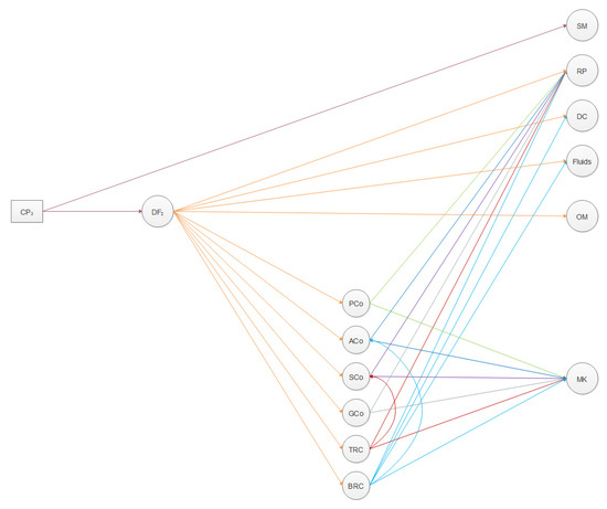
Figure 3. The optimal solution network proposed by the model with CP3, DF2, and the other entities. Burgundy, ELVs flow; orange, parts flow; green, plastics flow; dark blue, aluminum flow; purple, steel flow; solid gray, glass flow; red, tire flow; blue, battery flow.

It is notable that the amount of materials sent from the dismantling facility to processing facilities is a good amount, and they are profitable (over USD 4.3 million per year). The results are shown in Table 7, Table 8, Table 9 and Table 10. Figure 4 shows the amount of ELVs by type that are sent from CP to DF.

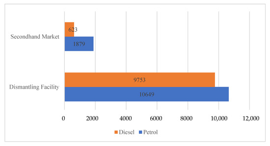
Figure 4. Amount of ELVs (by type) sent from collection points to dismantling facility and secondhand market.

On the other hand, Figure 5 illustrates the amount of different types of materials sent from DF to the other entities in the network. It is notable that steel is the largest amount of material sent from the DF. This emphasizes the proposed model to recycle ELVs and use the recycled materials instead of virgin materials.

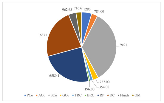
Figure 5. Total amount of materials from DF to other entities in the network (tonne/year).

The results show very interactive exchanges between the entities taking into consideration the CO₂ emission factor. The total amount of CO₂ emission for the network is 5688.64 tonnes CO₂ eq./year; this is equivalent to CO₂ emission from 6,287,560 pounds of coal burned according to the EPA greenhouse gas equivalent calculator [54]. The network saved CO₂ is 21,348.12 tonnes CO₂ eq./year, which is equivalent to CO₂ emission from 23,595,725 pounds of coal burned (according to the GHG Equivalencies Calculator) [54,55,56]. The detailed amount of saved CO₂ emission is illustrated in Figure 6.

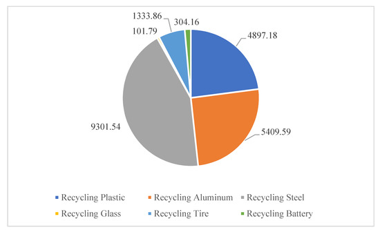
Figure 6. Saved CO₂ emissions by recycling different types of materials in the network (tonnes CO₂ eq./year).

3.3. Sensitivity Analysis

Variation of data causes different results that can be examined through sensitivity analyses. In order to address this issue, two sensitivity analyses are discussed to account for variations in key model parameters over the network’s economic and environmental performance. After carefully examining the previous results, it was noticed that two of the model parameters significantly influencing the operation of the proposed network are the number of ELVs processed in the network and the number of used vehicles send to the secondhand market. The first parameter represents the process material input, whereas the second accounts for the largest revenue contributor to the network’s economy.

As shown in Figure 7, the sensitivity to the number of ELVs was examined by increasing the total number of ELVs processed in the network from 100% (baseline) to 190% (i.e., 90% over the baseline). The baseline corresponds to the reference scenario discussed in the previous section. The 100–190% range comprises potential operating capacities for the network and sets the upper operating limit. Over this range, the problem becomes infeasible because the amount of steel recycled from ELVs becomes larger than the maximum intake capacity of recyclable steel set for the steel company.

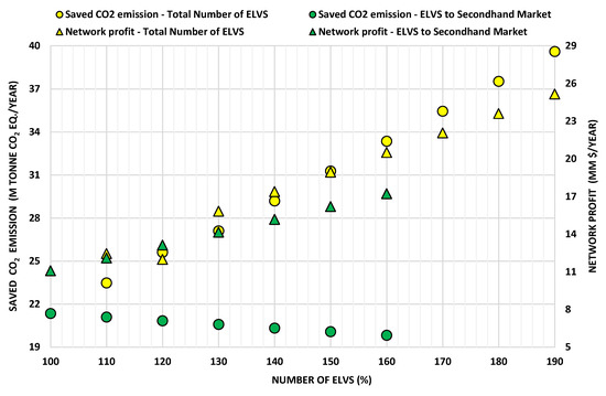
Figure 7. Saved CO₂ emission and network profit vs. number of ELVs (total and secondhand market).

Figure 7 shows in yellow color the saved CO₂ eq. emission (circle) and overall network profit (triangle) as a function of the total number of ELVs processed in the network. Accordingly, the greater the number of vehicles processed in the network the larger the CO₂ eq. emission savings when the comparison is to the number of vehicles to landfill. This is the direct result of larger amounts of recycled material being sent to the processing and recycling companies, replacing virgin materials, which have larger carbon footprints. Likewise, the network profit grows as the number of ELVs processed in the network expands. This is the result of higher numbers of used vehicles sold at the secondhand market and more material available to be recycled at processing/recycling companies, generating additional revenue. Accordingly, both variables are positively correlated with the number of ELVs processed in the network.

On the other hand, the sensitivity to the number of used vehicles sent to the secondhand market was studied by increasing the ELVs ratio to the market from 100% to 160%. This range comprises potential operating capacities for the secondhand market and also sets its upper operating limit. Beyond this upper limit, the problem becomes infeasible because the number of used vehicles sent to the secondhand market surpasses the maximum market capacity.

The green circle and triangle represent the saved CO₂ eq. emission and overall network profit as a function of the number of ELVs sent to the secondhand market, respectively. As shown in Figure 7, as the number of ELVs sent to the secondhand market grows, the CO₂ eq. emission savings decreases. This is because the number of ELVs available for dismantling is reduced, thus leading to less recycled materials that normally offset carbon footprints. Although the number of used vehicles sent to the secondhand market increases, the overall number of ELVs in the network is kept fixed.

Conversely, the network profit grows in line with the number of used vehicles sent to the secondhand market. This market is profitable; nonetheless, its profit growth rate is lower than that attained by increasing the total number of ELVs in the network (yellow triangle trend: first sensitivity analysis). Beyond the 120% operating point, a second dismantling facility is needed to process the increasing number of ELVs in the network. However, only where the number of ELVs equals 120%, the revenue generated by the materials processed in the second dismantling facility is not yet enough to offset the new associated dismantling expenses.

Even though the ratio of vehicles sent to the secondhand market remains unchanged for the sensitivity to the number of ELVs, as the total number of ELVs processed in the network grows, so indirectly does the number of used vehicles sent to the secondhand market. This translates into two different revenue streams for the network and explains its superior profit growth rate. Moreover, the CO₂ eq. emission savings variable is negatively correlated with the growing number of ELVs sent to the secondhand market, whereas the network profit is positively correlated.

4. Conclusions

The sustainable management of End-of-Life Vehicles (ELVs) has become a global priority due to the environmental concerns. Recycling and reusing materials is one solution to solve the problem of ELVs.

The research in this paper contributes to the scientific body of the knowledge by presenting a modeling framework in terms of a superstructure of alternatives, which takes into account full interactions between several entities. In addition, the research proposes a Mixed Integer Linear Programming model to find the optimal processing network while maximizing profit of the network

The proposed model was applied to a case study in Qatar. End-of-Life Vehicles in Qatar reach yearly more than 15,000 in number. The mathematical model consists of four nodes designed to operate as a network: collection points (i), dismantling facilities (j), processing facilities (k), and markets (m). The optimization procedure selects the most suitable combination of network components.

The results show that the model can process 30,715 tonnes/year from both types (petrol and diesel vehicles), which equals to 22,904 ELVs (12,528 petrol type, and 10,376 diesel type). In addition, the model shows that it is profitable to use the EIP-4-ELVs approach. The most reused material was steel. Notably, the total amount of CO₂ emission for the EIP-4-ELVs network is 5688.64 tonnes CO₂ eq./year, and the saved CO₂ is 21,348.12 tonnes CO₂ eq./year.

Overall, the model maximizes the total profit of the network and finds the amount of materials flow between the entities. In addition, the model decides which facility to open/use for the network flow. The results from the case study in Qatar can be directed to solve the issue of ELVs, as the number of ELVs is in rapid growth for many reasons. The area of Qatar being small helps the entities in the network to exchange by-products and wastes through the connected network. This connection will have a huge positive impact on economy, environment, and social aspects.

The economic side encourages profitable growth for the entities in the network while at the same time preventing the use of virgin materials to produce some essential products in the country. Hence, saving virgin materials will have impact on the environment by reducing the GHG emissions. In addition, the processing network allows and provides new jobs and opportunities for social growth in the community/country.

Future extended work for this model could include but should not be restricted to the following: new generation of vehicles (electric vehicles), uncertainty in the key model parameters, multi-period optimization, and parametric analysis using weight factors.

References

- United Nations. Arsenic and the 2030 Agenda for Sustainable Development. In Arsenic Research and Global Sustainability, Proceedings of the 6th International Congress Onarsenic in the Environment, Stockholm, Sweden, 19–23 June 2016; Routledge: Stockholm, Sweden, 2016. [Google Scholar]
- Ehrenfeld, J.; Gertler, N. Industrial Ecology in Practice: The Evolution of Interdependence at Kalundborg. J. Ind. Ecol. 1997, 1, 67–79. [Google Scholar] [CrossRef]
- Gómez, A.M.M.; González, F.A.; Bárcena, M.M. Smart eco-industrial parks: A circular economy implementation based on industrial metabolism. Resour. Conserv. Recycl. 2018, 135, 58–69. [Google Scholar] [CrossRef]
- De Almeida, S.T.; Borsato, M. Assessing the efficiency of End of Life technology in waste treatment—A bibliometric literature review. Resour. Conserv. Recycl. 2019, 140, 189–208. [Google Scholar] [CrossRef]
- Zhang, L.; Yuan, Z.; Bi, J.; Liu, B. Eco-industrial parks: National pilot practices in China. J. Clean. Prod. 2010, 18, 504–509. [Google Scholar] [CrossRef]
- Boix, M.; Montastruc, L.; Azzaro-Pantel, C.; Domenech, S. Optimization methods applied to the design of eco-industrial parks: A literature review. J. Clean. Prod. 2015, 87, 303–317. [Google Scholar] [CrossRef]
- Diener, D.L.; Tillman, A. Resources, Conservation and Recycling Scrapping steel components for recycling—Isn’t that good enough? Seeking improvements in automotive component end-of-life. Resour. Conserv. Recycl. 2016, 110, 48–60. [Google Scholar] [CrossRef]
- d’Ambrières, W. Plastics Recycling Worldwide: Current Overview and Desirable Changes. 2019. Available online: https://www.oneplanetnetwork.org/sites/default/files/from-crm/factsreports-5102.pdf (accessed on 1 August 2021).
- Saavedra, Y.M.B.; Iritani, D.R.; Pavan, A.L.R.; Ometto, A.R. Theoretical contribution of industrial ecology to circular economy. J. Clean. Prod. 2018, 170, 1514–1522. [Google Scholar] [CrossRef]
- Saidani, M.; Kendall, A.; Yannou, B.; Leroy, Y.; Cluzel, F. Management of the end-of-life of light and heavy vehicles in the U.S.: Comparison with the European union in a circular economy perspective. J. Mater. Cycles Waste Manag. 2019, 21, 1449–1461. [Google Scholar] [CrossRef]
- Despeisse, M.; Kishita, Y.; Nakano, M.; Barwood, M. Towards a circular economy for End-of-Life Vehicles: A comparative study UK–Japan. Procedia CIRP 2015, 29, 668–673. [Google Scholar] [CrossRef]
- Gu, C.; Leveneur, S.; Estel, L.; Yassine, A. Modeling and optimization of material/energy flow exchanges in an eco-industrial park. Energy Procedia 2013, 36, 243–252. [Google Scholar] [CrossRef]
- Chertow, M.R. Uncovering’ Industrial Symbiosis. J. Ind. Ecol. 2007, 11, 11–30. [Google Scholar] [CrossRef]
- Piaszczyk, C. Model Based Systems Engineering with Department of Defense Architectural Framework. Syst. Eng. 2011, 14, 305–326. [Google Scholar] [CrossRef]
- Behera, S.K.; Kim, J.H.; Lee, S.Y.; Suh, S.; Park, H.S. Evolution of ‘designed’ industrial symbiosis networks in the Ulsan Eco-industrial Park: ‘Research and development into business’ as the enabling framework. J. Clean. Prod. 2012, 29–30, 103–112. [Google Scholar] [CrossRef]
- Tessitore, S.; Daddi, T.; Iraldo, F. Eco-industrial parks development and integrated management challenges: Findings from Italy. Sustainability 2015, 7, 10036–10051. [Google Scholar] [CrossRef]
- Mat, N.; Cerceau, J.; Shi, L.; Park, H.S.; Junqua, G.; Lopez-Ferber, M. Socio-ecological transitions toward low-carbon port cities: Trends, changes and adaptation processes in Asia and Europe. J. Clean. Prod. 2016, 114, 362–375. [Google Scholar] [CrossRef]
- Aid, G.; Eklund, M.; Anderberg, S.; Baas, L. Expanding roles for the Swedish waste management sector in inter-organizational resource management. Resour. Conserv. Recycl. 2017, 124, 85–97. [Google Scholar] [CrossRef]
- Susur, E.; Hidalgo, A.; Chiaroni, D. A strategic niche management perspective on transitions to eco-industrial park development: A systematic review of case studies. Resour. Conserv. Recycl. 2019, 140, 338–359. [Google Scholar] [CrossRef]
- Chertow, M.R. Industrial symbiosis: Literature and taxonomy. Annu. Rev. Energy Environ. 2000, 25, 313–337. [Google Scholar] [CrossRef]
- Haskins, C. A Systems Engineering Framework for Eco–Industrial Park Formation. Syst. Eng. 2007, 10, 83–97. [Google Scholar] [CrossRef]
- Felicio, M.; Amaral, D.; Esposto, K.; Durany, X.G. Industrial symbiosis indicators to manage eco-industrial parks as dynamic systems. J. Clean. Prod. 2016, 118, 54–64. [Google Scholar] [CrossRef]
- European Parliament and Council. Directive 2000/53/EC on End-of-Life Vehicles. Off. J. Eur. Union 2000, L269, 34–42.
- Tian, J.; Chen, M. Sustainable design for automotive products: Dismantling and recycling of End-of-Life Vehicles. Waste Manag. 2014, 34, 458–467. [Google Scholar] [CrossRef] [PubMed]
- SIR. 2013 Steel Recycling Rates; SIR: Pittsburg, PA, USA, 2013. [Google Scholar]
- SRI. Steel Recycling Institute Turns 25; SRI: Pittsburgh, PA, USA, 2013. [Google Scholar]
- Sakai, S.; Yoshida, H.; Hiratsuka, J.; Vandecasteele, C.; Kohlmeyer, R.; Rotter, V.S.; Passarini, F.; Santini, A.; Peeler, M.; Li, J.; et al. An international comparative study of end-of-life vehicle (ELV) recycling systems. J. Mater. Cycles Waste Manag. 2014, 16, 1–20. [Google Scholar] [CrossRef]
- Vermeulen, I.; van Caneghem, J.; Block, C.; Baeyens, J.; Vandecasteele, C. Automotive shredder residue (ASR): Reviewing its production from End-of-Life Vehicles (ELVs) and its recycling, energy or chemicals’ valorisation. J. Hazard. Mater. 2011, 190, 8–27. [Google Scholar] [CrossRef] [PubMed]
- Li, Y.; Fujikawa, K.; Wang, J.; Li, X.; Ju, Y.; Chen, C. The potential and trend of end-of-life passenger vehicles recycling in China. Sustainability 2020, 12, 1455. [Google Scholar] [CrossRef]
- Saidani, M.; Yannou, B.; Leroy, Y.; Cluzel, F. Dismantling, remanufacturing and recovering heavy vehicles in a circular economy—Technico-economic and organisational lessons learnt from an industrial pilot study. Resour. Conserv. Recycl. 2020, 156, 104684. [Google Scholar] [CrossRef]
- Soo, V.K.; Peeters, J.; Compston, P.; Doolan, M.; Duflou, J.R. Comparative Study of End-of-Life Vehicle Recycling in Australia and Belgium. Procedia CIRP 2017, 61, 269–274. [Google Scholar] [CrossRef]
- Karagoz, S.; Aydin, N.; Simic, V. End-of-life vehicle management: A comprehensive review. J. Mater. Cycles Waste Manag. 2020, 22, 416–442. [Google Scholar] [CrossRef]
- Simic, V.; Branka, D.S.; Branislava, R.V. Closed-Loop Supply Chain of End-of-Life Vehicles. In Proceedings of the XIX International Conference on Material Handling, Constructions and Logistics’09, Belgrade, Serbia, 15–16 October 2009; pp. 189–194. [Google Scholar]
- Özceylan, E.; Demirel, N.; Çetinkaya, C.; Demirel, E. A closed-loop supply chain network design for automotive industry in Turkey. Comput. Ind. Eng. 2017, 113, 727–745. [Google Scholar] [CrossRef]
- Demirel, E.; Demirel, N.; Gökçen, H. A mixed integer linear programming model to optimize reverse logistics activities of End-of-Life Vehicles in Turkey. J. Clean. Prod. 2016, 112, 2101–2113. [Google Scholar] [CrossRef]
- Simic, V. End-of-life vehicle recycling-a review of the state-of-the-art. Recikliranje Vozila Kraj. Životnog Ciklusa-Pregl. Najsuvremnijih Znan. Rad. 2013, 20, 371–380. [Google Scholar]
- Planning and Statistics Authority. Quarterly Bulletin Population Statistics; Planning and Statistics Authority: Doha, Qatar, 2020.
- Al-quradaghi, S.; Zheng, Q.P.; Elkamel, A. Generalized Framework for the Design of Eco-Industrial Parks: Case Study of End-of-Life Vehicles. Sustainability 2020, 12, 6612. [Google Scholar] [CrossRef]
- Rogers, D.S.; Tibben-Lembke, R.S. Going Backwards: Reverse Logistics Trends and Practices; Reverse Logistics Executive Council: Pittsburgh, PA, USA, 1999. [Google Scholar]
- Kuşakcı, A.O.; Ayvaz, B.; Cin, E.; Aydın, N. Optimization of reverse logistics network of End of Life Vehicles under fuzzy supply: A case study for Istanbul Metropolitan Area. J. Clean. Prod. 2019, 215, 1036–1051. [Google Scholar] [CrossRef]
- Simic, V. A multi-stage interval-stochastic programming model for planning End-of-Life Vehicles allocation. J. Clean. Prod. 2016, 115, 366–381. [Google Scholar] [CrossRef]
- Choi, J.; Stuart, J.A.; Ramani, K. Modeling of Automotive Recycling Planning in the United States. Int. J. Automot. Technol. 2005, 6, 413–419. [Google Scholar]
- Simic, V.; Dimitrijevic, B. Interval linear programming model for long-term planning of vehicle recycling in the Republic of Serbia under uncertainty. Waste Manag. Res. 2015, 33, 114–129. [Google Scholar] [CrossRef]
- van Schaik, A.; Reuter, M.A. The optimization of end-of-life vehicle recycling in the European Union. JOM 2004, 56, 39–43. [Google Scholar] [CrossRef]
- Phuc, P.N.K.; Yu, V.F.; Tsao, Y.C. Optimizing fuzzy reverse supply chain for End-of-Life Vehicles. Comput. Ind. Eng. 2017, 113, 757–765. [Google Scholar] [CrossRef]
- D’Adamo, I.; Gastaldi, M.; Rosa, P. Recycling of End-of-Life Vehicles: Assessing trends and performances in Europe. Technol. Forecast. Soc. Chang. 2020, 152, 119887. [Google Scholar] [CrossRef]
- Cruz-rivera, R.; Ertel, J. Reverse logistics network design for the collection of End-of-Life Vehicles in Mexico. Eur. J. Oper. Res. 2009, 196, 930–939. [Google Scholar] [CrossRef]
- Cin, E.; Kusakcı, A.O. A Literature Survey on Reverse Logistics of End of Life Vehicles. Southeast Eur. J. Soft Comput. 2017, 6, 31–39. [Google Scholar] [CrossRef][Green Version]
- ARDP. Auto Recycling Demonstration Project; ARDP: Ann Avbobr, MI, USA, 1998. [Google Scholar]
- Edwards, C.; Bhamra, T.; Rahimifard, S. A Design Framework for End-of-Life Vehicle Recovery. In Proceedings of the 13th CIRP International Conference on Life Cycle Engineering, Leuven, Belgium, 31 May–2 June 2006; pp. 365–370. [Google Scholar]
- Wang, L.U.; Chen, M. End-of-Life Vehicle Dismantling and Recycling Enterprises: Developing Directions in China. JOM 2017, 65, 1015–1020. [Google Scholar] [CrossRef]
- ARA. Automotive Recycling Industry: Environmentally Friendly, Market Driven, and Sustainable; ARA: Manassas, VA, USA, 2012. [Google Scholar]
- Cassells, S. Toward Sound Management of End-of-Life Vehicles in New Zealand; Massey University: Palmerston, New Zealand, 2004. [Google Scholar]
- Yu, C.; de Jong, M.; Dijkema, G.P.J. Process analysis of eco-industrial park development-The case of Tianjin, China. J. Clean. Prod. 2014, 64, 464–477. [Google Scholar] [CrossRef]
- Kumar, S.; Yamaoka, T. System dynamics study of the Japanese automotive industry closed loop supply chain. J. Manuf. Technol. Manag. 2007, 18, 115–138. [Google Scholar] [CrossRef]
- Ahmed, S.; Ahmed, S.; Shumon, M.; Quader, M. End-of-Life Vehicles (ELVs) Management and Future Transformation in Malaysia. J. Appl. Sci. Agric. 2014, 9, 227–237. [Google Scholar]
Publisher’s Note: MDPI stays neutral with regard to jurisdictional claims in published maps and institutional affiliations. |
© 2022 by the authors. Licensee MDPI, Basel, Switzerland. This article is an open access article distributed under the terms and conditions of the Creative Commons Attribution (CC BY) license (https://creativecommons.org/licenses/by/4.0/).