Trade Openness and Environmental Policy Stringency: Quantile Evidence

Abstract

The intensively debated issue of whether trade globalization leads to a race (climb) to the bottom (top) such that environmental policy stringency is loosened (strengthened) is still far from being uncontroversial. This paper provides new empirical evidence from the standpoint of the North (advanced) countries using both the generalized methods of moment (GMM) and GMM quantile estimators for dynamic panel data models. It first investigates the importance of trade partners and finds, in a sample of OECD countries, that increased trade with the South (developing) countries leads to more stringent environmental regulation whereas heightened trade with the North eases environmental regulation. It then examines whether there exist differences across regimes with different extents of stringency in environmental regulation and finds significant regime-specific effects. Specifically, liberalizing trade with the North weakens environmental regulation stringency in a regime with medium stringency but reinforces it in a regime with high and low stringency. Conversely, expanded trade with the South raises environmental regulation stringency in a regime with medium stringency but deteriorates it in a regime with high and low stringency.

1. Introduction

Environmental policy or regulation is considered one effective route to contain environmental pollution. Such a belief is rooted in the environmental Kuznets curve hypothesis, according to which economic growth increases social demand for environmental protection and stringent environmental policy that improve the environmental quality [1]. Thus, stringent environmental policy has the feature of making possible the coexistence of economic growth and better environmental quality. It is thus interesting to know what determines environmental policy stringency.

Trade openness is often regarded as one crucial determinant of environmental policy stringency. When facing intensive foreign competition due to greater trade openness, governments of countries with more stringent pollution control may be inclined to loosen it so as to protect domestic industries and employment. However, stricter environmental policy can create incentives for firm innovation toward clean and energy-efficient technology to reduce production costs, particularly so when facing greater market size and profitable opportunities that come with trade liberalization. Such policy-induced green innovation has been seen as the most powerful mechanism for environmental policy to reduce pollution and promote the support of stringent environmental policy. Thus, there is no clear-cut of whether trade leads to a race to the bottom (i.e., loose policy) or climbs to the top (i.e., strict policy).

While there are intensive theoretical debates about how trade is linked to environmental policy stringency, empirical investigations are still relatively sparse. Perhaps it is because of lacking accurate data on environmental regulation comparable across countries and over time. To close the void, this paper revisits the issue and adds new evidence from the standpoint of North countries using a newly constructed index for environmental regulation from the OECD statistics. The index is derived from information on selected environmental policy instruments, mostly related to climate and air pollution to create a composite measure of relative policy stringency across (mostly OECD) countries and over time [2]. Our focus on the North countries is motivated by the following observations, in addition to data limitation. The North countries have the capacity to innovate, implement, and adopt new technology, meaning that their trade particularly with the South countries enables them to explore the first-mover advantage. It is also argued that North countries have an incentive to use environmental policy to tilt the competitive relationship in favor of domestic firms and restrict the market access of foreign firms, particularly when trading with developing countries [3].

The paper contributes to the current empirical literature mainly in two aspects. First, it differentiates the direction of trade between advanced (North) and developing (South) countries, which enables analysis in a North–North and North–South context, similarly to Aklin [4] and Kim et al. [5]. Among the North countries, the dominant form of trade is the international exchange of varieties of differentiated products within the same industry. Such intra-industry trade arises to take advantage of scale economies in production and/or reflect demand for product variation and hence tends to encourage the diffusion of clean technology and green best practices. On the contrary, North–South trade usually involves the global exchange of different products based on their comparative advantage (for instance, relative factor abundance and environmental regulation), and thus tends to promote outsourcing. As such, the analysis of differentiating high- and low-income trading partners can provide insight into trade’s influence on stringency in environmental regulation.

Second, we explore whether trade affects environmental regulation differently across regimes with various degrees of environmental stringency. This is critical. According to the race to the bottom thesis, trade competition among countries with wide disparities in stringency and standards will exert downward pressure on standards and strictness in the countries with higher stringent standards. However, as put forth by Porter [6], it is in the countries with lower stringency that competitiveness concerns exert downward pressure on standards and stringency because these countries have weaker environmental governance and greater dependence on low-cost manufacturing (i.e., low-cost production technologies with higher emission intensities) to maintain international competitiveness. Thus, low-regulated countries remain stuck at the bottom in a regime of free trade. From a policy perspective, it is therefore interesting to learn about the behavior of environmental regulation at different levels of stringency.

Methodologically, we first consider the dynamic panel system GMM estimator to control for endogeneity due to reverse causation and the omitted-variable bias. However, GMM provides estimates at the conditional mean of the environmental regulation stringency distribution and captures only the central tendency of effects. We then consider the dynamic panel GMM quantile model. The quantile approach gives one estimate for each quantile of the entire conditional distribution of environmental regulation stringency. This methodology enables us to address the consequences of trade on environmental regulation stringency throughout the conditional distribution, with particular focus on those countries with the least and most regulation stringency.

The following sections provide a brief review of the literature (Section 2), discuss the data and model specifications as well as estimation strategies (Section 3), conduct estimations and discuss the results (Section 4), and conclude the paper (Section 5).

2. A Brief Review of Literature

A long-debated issue of whether trade globalization leads to a race (climb) to the bottom (top) such that environmental policy stringency is loosened (strengthened) is still far from being uncontroversial (e.g., [7,8] for a comprehensive review and references therein). Conventional wisdom holds that environmental regulation imposes significant production costs and slows productivity growth, which hinders the capacity of firms to compete in international markets or even leads to the migration of pollution-intensive production from countries with stringent environmental regulation to those with lax stringent regulation. Thus, the concern over potential competitiveness loss due to trade liberalization may place downward pressure on standards and stringency of environmental regulation, leading to the so-called regulatory chill or even a race to the bottom [9,10]. However, it is argued that if properly designed and implemented, more stringent environmental regulation could promote cost-saving efficiency development and encourage firm innovation toward green technology, both of which may lead not only to neutralizing the regulation’s initial costs but also to increasing international competitiveness [11]. Thus, trade may actually lead to more stringency in environmental regulation. Environmental regulation could also act as a trade barrier, causing a climb to the top in standards and stringency [3].

Still, several recent studies, based on a political economy approach, postulate that the trade’s effect on environmental regulation depends on the size of the relative shifts in the political power of industrial and environmental lobby groups, which is further determined by a country’s comparative (dis)advantage in the polluting sector [12,13], the extent of substitution between foreign and domestic goods [14], the distribution of production factor ownership [15], who, producers or consumers, ultimately generates pollution [16], domestic political constraints, and the issue visibility of the pollutant [17], or quality and structure of political institutions [18,19]. It is thus not clear ex ante whether, and to what extent, trade would influence environmental regulation stringency.

On the empirical front, the literature contains relatively little work due in large part to a shortcoming of available cross-country data on environmental policy. Even with limited studies, there is no conclusive evidence on the impact of trade on local environmental regulation. For instance, Ederington and Minier [3] investigate environmental compliance costs within US manufacturing industries and find that environmental policies act as a secondary trade barrier in the U.S. and that a lower tariff rate is associated with stricter environmental regulation. Similarly, using data on countries’ initial adoption year of comprehensive automobile emission standards from a sample of developed and developing countries, Saikawa [20] finds that trade encourages a race to the top in environmental standards and regulation. Prakash and Potoski [21] demonstrate that trade linkages encourage ISO 14,001 adoption if countries’ major export markets have adopted this voluntary regulation in a sample of developed and developing countries. By contrast, using surveys on the perceptions of stringency, Busse and Silberberger [22] show that an increase in the net exports of pollution-intensive goods leads to less stringent environmental regulation in a cross-country context.

Nonlinearity is also found. Aisbett and Silberberger [23] examine sanitary and phytosanitary notifications for a sample of developed and developing countries and find that trade liberalization leads to a race to the top among high-standard countries but a regulatory-chill effect among low-standard countries. Likewise, Damaia et al. [24] employ fuel quality standards such as the lead content of gasoline and find that trade liberalization decreases (increases) environmental policy strictness for countries with low (high) corruption.

Along the same line, instead of verifying whether trade strengthens or eases environmental policy stringency, the paper takes one step further to explore the potential importance of trade partners and (quantile) heterogeneity in the relationship, which may shed some light on theoretical inconclusiveness.

3. Data and Methodology

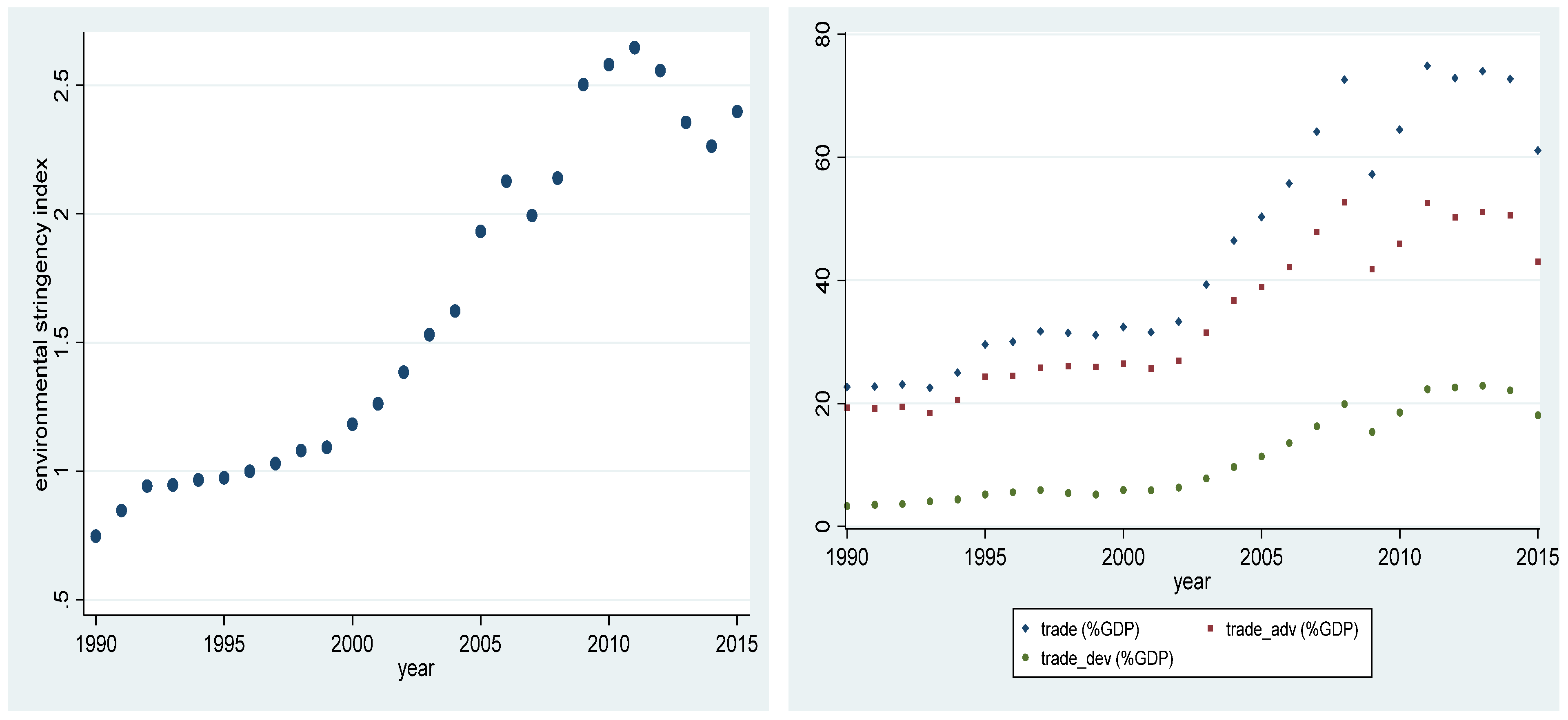
3.1. Data

The lack of accurate data to measure environmental regulation has remained one of the main difficulties faced by most empirical studies to date. While attempts to measure environmental policy stringency across countries have been undertaken in the past, the lack of a sufficient time-series dimension has limited their empirical application. This paper considers the environmental policy stringency index sourced from the OECD database The index is a country-specific and internationally comparable measure of stringency in environmental policy. Stringency is defined as the extent to which environmental policies place an explicit or implicit price on polluting or environmentally harmful behavior. The policies include environmentally related taxes, renewable energy and energy efficiency support, performance standards, and information on deposit and refund schemes. Currently, the indicator focuses mainly on air and climate policies. The index ranges from 0 (not stringent) to 6 (highest degree of stringency) and covers 28 OECD and 6 BRIICS countries for the period 1990–2015. In the study, we include 27 OECD countries for which we have at least two-thirds of the observations during the period 1990–2015. These include Australia, Austria, Belgium, Canada, Czech Rep., Denmark, Finland, France, Germany, Greece, Hungary, Ireland, Italy, Japan, Korea, Rep., Netherlands, Norway, Poland, Portugal, Slovak Rep., Slovenia, Spain, Sweden, Switzerland, Turkey, the United Kingdom, and the United States. It is very common in the empirical macro literature to transform annual data into non-overlapping 4 or 5 year periods during the sample period to mitigate business fluctuation effects and measurement errors. Since we have a shorter time period, we consider non-overlapping 3-year averaged data except for the last period which is a 2-year period, i.e., 1990–1992, 1993–1995, 1996–1998, 1999–2001, 2002–2004, 2005–2007, 2008–2010, 2011–2013, and 2014–2015.

Regarding trade openness, as typical in the empirical literature, we first consider trade intensity, the sum of exports and imports as a share of GDP. We then consider trade intensity at the disaggregate level. These include trade with North countries ($trade\_N$), the sum of exports to and imports from advanced countries as a percentage of GDP, and trade with South countries $\left(trade\_S\right),$ the sum of exports to and imports from developing countries as a percentage of GDP. As a robustness check, we also experiment with imports from North countries as a share of GDP ($import\_N$), imports from South countries as a share of GDP ($import\_S$), exports to North countries as a share of GDP ($export\_N$), and exports to South countries as a share of GDP ($export\_S$). All trade variables are sources from the IMF Direction of Trade Statistics and in logs.

To alleviate the omitted-variable bias, we include control variables together with country- and time-specific dummies following the prior empirical literature (see, e.g., Eliste and Fredriksson [25]; Lisciandra and Migliardo [26]; Dincer and Fredrikssonb [27]). These are GDP per capita and its squared term to control for income-induced environmental policy responses: income gains due to economic growth make pollution policy more stringent, which alleviates environmental pollution [27]. The inclusion of FDI flows as a share of GDP is based on the pollution haven hypothesis: the government may implement lax environmental policies so as to attract foreign capital [28,29]. Added is the share of internet users in the total population to capture the effect of information flows. The internet provides not only greater access to publicly available information about climate change and environmentalism as well as local environmental quality but also the opportunity to respond and participate immediately, which could enhance the strength of governments to implement decent environmental standards and regulations [30]. Data on these variables are taken from the World Development Indicators of the World Bank and in logs. Control of corruption is included to account for the corruption effect: less corruption means a greater weight on social welfare and hence more stringent environmental policy [19,31]. Data on control of corruption are sourced from the Worldwide Governance Indicators of the World Bank, with the value ranging from −2.5 to 2.5. It measures the extent to which public power is practiced for private benefits, including both petty and grand forms of corruption, as well as the capture of the state by elites and private interests.

Table 1. Descriptive statistics.

	EPS	trade	trade_N	trade_S	export_N	export_S	import_N	import_S	FDI	GDP Per Capita	Internet Use	Control of Corruption
	Panel A: Summary statistics
obs.	258	260	260	260	260	260	260	260	263	264	262	231
mean	1.649	3.574	3.265	2.088	2.568	1.302	2.543	1.442	1.179	9.935	2.314	1.022
std.dev.	0.96	0.695	0.752	0.771	0.799	0.809	0.767	0.794	0.993	1.05	2.447	0.969
min	0.333	1.6	1.166	0.556	0.643	−0.271	−0.033	−0.214	−2.34	6.381	−8.711	−1.176
max	4.028	5.164	4.998	3.915	4.338	3.283	4.27	3.216	4.062	11.416	4.561	2.436
	Panel B: Pairwise correlations
EPS	1
trade	0.621 *	1
trade_N	0.577 *	0.577 *	1
trade_S	0.573 *	0.573 *	0.573 *	1
export_N	0.540 *	0.540 *	0.540 *	0.581 *	1
export_S	0.529 *	0.529 *	0.529 *	0.960 *	0.960 *	1
import_N	0.582 *	0.582 *	0.582 *	0.599 *	0.599 *	0.599 *	1
import_S	0.570 *	0.570 *	0.570 *	0.972 *	0.972 *	0.972 *	0.588 *	1
FDI	0.244 *	0.244 *	0.244 *	0.182 *	0.182 *	0.182 *	0.511 *	0.511 *	1
GDP per capita	0.572 *	0.572 *	0.572 *	0.075	0.075	0.075	0.413 *	0.413 *	0.413 *	1
internet use	0.549 *	0.549 *	0.549 *	0.403 *	0.403 *	0.403 *	0.343 *	0.343 *	0.343 *	0.343 *	1
control of corruption	0.505 *	0.505 *	0.505 *	−0.124	−0.124	−0.124	0.382 *	0.382 *	0.382 *	0.382 *	0.382 *	1

Note: All variables are in logs except for environmental policy stringency and control of corruption. * shows significance at the 5% level.

reports summary statistics and the correlation matrix. Figure 1 displays the scatter plot of the data averaged across countries over the period 1990–2015.

3.2. Model Specifications

We estimate the impact of trade $\left(trade\right)$ on environmental policy stringency $\left(EPS\right)$ based on the following dynamic panel regression model as Busse and Silberberger [22]:

$$EP{S}_{it}=\rho EP{S}_{it-1}+{\beta }_{1}trad{e}_{it}+{\gamma }^{\prime }C{V}_{it-1}+{\alpha }_i+d_t+{\epsilon }_{it}$$

(1)

where the country index $i=1, 2,\dots , N$ and the period indicator $t=1, 2,\dots ,T$. The country-specific effects ${\alpha }_i$ capture important heterogeneity across countries that would be left uncontrolled in a standard cross-sectional model and the time effects $d_t$ capture any factors that are dynamic but affect the level of environmental stringency, such as global preference changes due to education and technology. ${\epsilon }_{it}$ is the error term and assumed to be independently and identically distributed. $CV$ is a set of control variables. We lag one-period $CV$ to mitigate the endogeneity bias.

To further check for the potential difference between trade with advanced and developing countries, we then estimate the following dynamic panel equations:

$$EP{S}_{it}=\rho EP{S}_{it-1}+{\beta }_{1}trade\_N_{it}+{\beta }_{2}trade\_S_{it}+{\gamma }^{\prime }C{V}_{it-1}+{\alpha }_i+d_t+{\epsilon }_{it}$$

(2)

$$EP{S}_{it}=\rho EP{S}_{it-1}+{\beta }_{1}export\_N_{it}+{\beta }_{2}export\_S_{it}+{\gamma }^{\prime }C{V}_{it-1}+{\alpha }_i+d_t+{\epsilon }_{it }$$

(3)

$$EP{S}_{it}=\rho EP{S}_{it-1}+{\beta }_{1}import\_N_{it}+{\beta }_{2}import\_S_{it}+{\gamma }^{\prime }C{V}_{it-1}+{\alpha }_i+d_t+{\epsilon }_{it}$$

(4)

The above equations are subject to the endogeneity problem due to (i) the omitted-variable bias: the observed relationship between environmental policy stringency and trade variables may be driven by government preferences and political institutions; (ii) reverse causality: polluting industries prefer inefficient environmental policy instruments because they increase the level of trade barriers; (iii) the presence of lagged dependent variables. We then estimate these equations using the system GMM estimator developed by Arellano and Bover [31] and Blundell and Bond [32] for dynamic panels. Apart from accounting for dynamics, the estimator accommodates the potential endogeneity between environmental policy stringency and trade variables via appropriate instruments. The system GMM is derived from the estimation of a system of two simultaneous equations: one in levels (with lagged first differences as instruments) and the other in first differences (with lagged levels as instruments). It is also noted that due to the small size of our sample, we do not consider external instruments but these internal ones.

The consistency of the system GMM estimator depends on two specification tests. The first one is the Hansen J test of over-identifying restrictions. The failure to reject the null of the Hansen J test implies that the instruments are valid and the model is correctly specified. A first step in the estimation process is to take the first difference on the level equation so as to remove the fixed effect. However, this may introduce the correlation between differenced error terms $\Delta {\epsilon }_{it}$ and differenced one-period lagged dependent variable, $\Delta EP{S}_{it-1}$. Thus, the second one is to test serial correlation in the first-differenced errors. If the error term in levels is serially uncorrelated, this means that the error term in first differences has a negative first-order serial correlation but no second-order serial correlation. One should therefore reject the null hypothesis of no first-order serial correlation in first differences (AR(1) test) but should not reject the null hypothesis of no second-order serial correlation in first differences (AR(2) test). These tests, however, lose power when the number of instruments is large relative to the cross-section sample size. We then follow Roodman [33] to collapse the instruments and limit their number. Given the small size of our sample, we use the small-sample corrected standard errors proposed by Windmeijer [34] to reduce the small-sample bias.

The above equations assume parameter homogeneity and look exclusively at the trade effect on the mean of the environmental policy stringency distribution. To allow for the existence of quantile parameter heterogeneity and hence explore how trade flows influence environmental policy stringency at different quantiles of the environmental policy stringency distribution, we consider the dynamic panel GMM quantile model with non-additive fixed effects advanced by Powell and Wagner [35] and Powell [36]. Typically, the quantile estimators with additive fixed effects provide estimates of the conditional distribution of environmental policy stringency relative to fixed effect $(EP{S}_{it}-{\alpha }_i).$ Yet, this approach produces estimates of the conditional distribution of $EP{S}_{it},$ in the same way as cross-sectional quantile estimates. This is performed by including the fixed effects in the error term and then estimating the panel quantile regression via GMM estimators to address endogeneity in the relationship.

Specifically, we estimate the conditional quantile function for quantile $q$ as follows:

$$Q_{EP{S}_{it}}\left(q_k|d_t,x_{it}\right)=d_t+b_{1q}EP{S}_{it-1}+b_{2q}trad{e}_{it}+{b^{\prime }}_{4q}C{V}_{it-1}$$

(5)

$$Q_{EP{S}_{it}}\left(q_k|d_t,x_{it}\right)=d_t+b_{1q}EP{S}_{it-1}+b_{2q}trade\_N_{it}+b_{3q}trade\_S_{it}+{b^{\prime }}_{4q}C{V}_{it-1}$$

(6)

$$Q_{EP{S}_{it}}\left(q_k|d_t,x_{it}\right)=d_t+b_{1q}EP{S}_{it-1}+b_{2q}export\_N_{it}+b_{3q}export\_S_{it}+{b^{\prime }}_{4q}C{V}_{it-1}$$

(7)

$$Q_{EP{S}_{it}}\left(q_k|d_t,x_{it}\right)=d_t+b_{1q}EP{S}_{it-1}+b_{2q}import\_N_{it}+b_{q3}import\_S_{it}+{b^{\prime }}_{4q}C{V}_{it-1}$$

(8)

It is noted that $b_{kq}$ measures the marginal effect of the kth explanatory variable on environmental policy stringency at the $q\mathrm{th}$ quantile. To estimate the quantile coefficient, Powell introduces estimation methods based on the conditional moment restrictions:

$$\left\{\frac{1}{T}{\displaystyle \sum }_t^T\left(w_{it}-{\overline{w}}_i\right)\left[1\left(EP{S}_{it}\le {x^{\prime }}_{it}B\left(q\right)\right)\right]\right\}=0$$

(9)

and

$$E\left[1\left(EP{S}_{it}\le {x^{\prime }}_{it}B\left(q\right)\right)-q\right]=0$$

(10)

for each $q\in \left(0,1\right)$, where ${x^{\prime }}_{it}$ is a vector of trade and control variables as well as lagged EPS with the corresponding quantile coefficient $B\left(q\right)$ and $w_i=(w_{i1}, w_{i2},$ …, $w_{iT})$ is a set of instruments. Equation (9) implies that identification originates from within-individual variation in the instruments $\left(w_{it}-{\overline{w}}_i\right)$ and Equation (10) states that the probability for $EP{S}_{it}$ to be smaller than the quantile function ${x^{\prime }}_{it}B\left(q\right)$ is equal to $q$ for all $t$.

Define sample moments using $\widehat{g}\left(b\right)=\frac{1}{N}{\displaystyle \sum }_{i=1}^N{g}_i\left(b\right) \mathrm{with} g_i\left(b\right)=\frac{1}{T}{\displaystyle \sum }_{t=1}^T\left(w_{it}-{\overline{w}}_i\right)\left[1\left(EP{S}_{it}\le {x^{\prime }}_{it}B\left(q\right)\right)\right]$ and constrain estimated parameters to $B=\left\{b|q-\frac{1}{N}<\frac{1}{N}{\displaystyle \sum }_{i=1}^{N}1\left(EP{S}_{it}\le {x^{\prime }}_{it}\right)\le q \mathrm{for} \mathrm{all} t\right\}$, a GMM estimator for $B\left(q\right)$ is $\widehat{B\left(q\right)}=argmi{n}_{b\in B}\widehat{g}{\left(b\right)}^{\prime }\widehat{A}\widehat{g}\left(b\right)$ for some weighting matrix $A$. Two-step GMM estimation can be employed for identification. Please refer to Powell [36] and Kim et al. [5] for discussions.

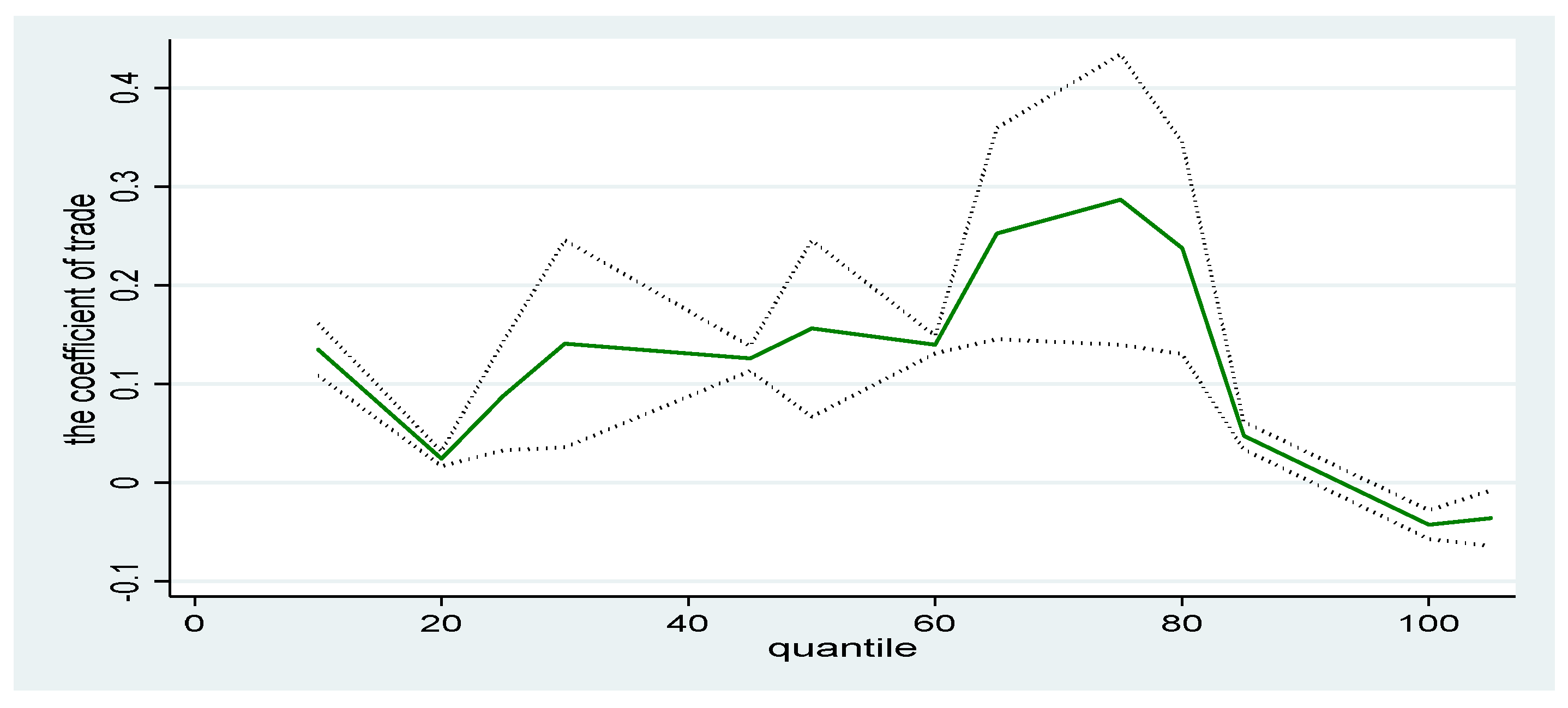
4. Empirical Results

Table 2. GMM estimates, aggregate data on trade flows.

	(1)	(2)	(3)	(4)	(5)
environmental policy stringency t−1	0.166 ***	0.113 ***	0.156 ***	0.271 ***	0.630 ***
	(0.040)	(0.038)	(0.051)	(0.044)	(0.070)
trade	1.642 ***	1.652 ***	1.698 ***	1.451 ***	0.360 ***
	(0.118)	(0.107)	(0.121)	(0.116)	(0.122)
GDP per capita t−1	−2.521	−2.571	−2.916 *	−0.529	−1.476
	(1.644)	(1.633)	(1.617)	(1.159)	(1.178)
squared GDP per capita t−1	0.145 *	0.152 *	0.169 **	0.061	0.080
	(0.082)	(0.080)	(0.079)	(0.058)	(0.060)
FDI t−1		−0.103 ***	−0.092 ***	−0.066 ***	−0.090 ***
		(0.016)	(0.028)	(0.022)	(0.031)
internet use t−1			−0.024	−0.049	−0.025
			(0.015)	(0.031)	(0.022)
control of corruption t−1				−0.161	−0.005
				(0.133)	(0.054)
period dummies					yes
constant	6.006	5.999	7.514	−4.588	4.511
	(8.215)	(8.327)	(8.195)	(5.687)	(5.607)
instrument count	21	22	22	23	23
AR(1)	−1.76 *	−1.74 *	−1.74 *	−2.42 **	−2.91 ***
	[0.078]	[0.081]	[0.081]	[0.016]	[0.004]
AR(2)	−1.58	−1.39	−1.45	−1.42	−1.19
	[0.115]	[0.166]	[0.148]	[0.155]	[0.234]
Hansen J	21.33	20.98	0.154	9.59	15.37
	[0.166]	[0.179]	[20.50]	[0.188]	[0.285]
obs.: N × T (N)	207 (27)	207 (27)	207 (27)	182 (27)	182 (27)

Note: The dependent variable is environmental policy stringency. One-period (three years) lagged explanatory variables are used as instruments for quantile estimation. Standard errors (p-values) are in parentheses (brackets). *** p < 0.01, ** p < 0.05, * p < 0.1.

provides the benchmark estimation results from GMM. As observed, the estimated regression is correctly specified. The Hansen J test indicates that the estimated equation is not overidentified and the null hypothesis of the absence of second-order serial correlation is not rejected. Moreover, the instrument count is smaller than the number of countries. Moving to the estimate of particular interestacross regressions, trade has a positive and significant effect on environmental policy stringency, supporting the climb to the top hypotheses, consistent with Damania et al. [19]. The rationale could arise because the governments of OECD countries are more responsive to demand for environmental improvements and/or because stricter environmental regulation improves the international competitiveness of OECD countries by driving enterprise innovation toward technologies that protect the environment or produce less environmental damage, whereas the compliance costs are negligible. This could be the reason that environmental regulation in OECD countries tends to be restricted relative to developing countries.

Table 3. Quantile estimates, aggregate data on trade flows.

		Quantile
	GMM	10th	25th	50th	75th	90th
environmental policy stringency t−1	0.630 ***	0.795 ***	0.688 ***	0.690 ***	0.525 ***	0.515 ***
	(0.070)	(0.022)	(0.004)	(0.022)	(0.017)	(0.004)
trade	0.360 **	0.135 ***	0.088 ***	0.156 ***	0.287 ***	−0.042 ***
	(0.152)	(0.013)	(0.028)	(0.046)	(0.075)	(0.007)
GDP per capita t−1	−1.476	−0.668 ***	0.656 ***	−1.271 ***	−1.313 ***	0.801 ***
	(1.178)	(0.207)	(0.055)	(0.393)	(0.212)	(0.041)
squared GDP per capita t−1	0.080	0.039 ***	−0.034 ***	0.067 ***	0.055 ***	−0.040 ***
	(0.061)	(0.010)	(0.003)	(0.019)	(0.013)	(0.002)
FDI t−1	−0.090 **	0.015 *	0.006 **	0.070 ***	0.045 ***	0.003
	(0.038)	(0.008)	(0.003)	(0.009)	(0.004)	(0.004)
internet use t−1	−0.025	−0.242 ***	−0.079 ***	−0.032 ***	0.234 ***	0.072 ***
	(0.022)	(0.060)	(0.002)	(0.004)	(0.012)	(0.003)
control of corruption t−1	−0.005	0.119 ***	0.160 ***	0.030 **	0.108 **	0.101 ***
	(0.054)	(0.014)	(0.004)	0.690 ***	(0.047)	(0.007)
constant	4.511
	(5.607)
instrument count	23
AR(1)	−2.91 ***
	[0.004]
AR(2)	−1.19
	[0.234]
Hansen J test statistic	15.37
	[0.285]
Obs.: N × T (N)	182 (27)	182 (27)	182 (27)	182 (27)	182 (27)	182 (27)

Note: The dependent variable is environmental policy stringency. Period dummies are included. One-period (three years) lagged explanatory variables are used as instruments for quantile estimation. Standard errors (p-values) are in parentheses (brackets). *** p < 0.01, ** p< 0.05, * p < 0.1.

reports the estimates for the 10th, 25th, 50th, 75th, and 90th quantile. For comparison purposes, we also report the GMM estimates for the full control variables (i.e., the Column (5) regression of Table 2). These quantile estimates further suggest that the climb-to-the-top effect seems to hold across quantiles, except for the 90th quantile where trade turns negative and significant. Figure 2 reports the corresponding quantile estimates of trade with 95% confidence intervals. In contrast with Aisbett and Silberberger [24], greater trade openness eases stringency in environmental regulation of the most stringent OECD countries, implying the dominance of the race to the bottom effect in a regime with most regulation stringency. The evidence lends support to the argument for upward harmonization of environmental regulation that the most regulated countries tend to ease their environmental regulation in a regime of free trade [6], possibly because for the most regulated OECD countries, strict environmental regulation has not significantly promoted technological innovation and has not brought enterprises enough benefits to make up for the environmental compliance cost.

Table 4. GMM and quantile estimates, disaggregate data on trade flows.

		Quantile
	GMM	10th	25th	50th	75th	90th
environmental policy stringency t−1	0.233 ***	0.770 ***	0.693 ***	0.661 ***	0.633 ***	0.544 ***
	(0.053)	(0.014)	(0.007)	(0.005)	(0.004)	(0.003)
trade with advanced countries	−0.193 **	0.165 ***	−0.048 ***	−0.146 ***	−0.042 ***	0.017 ***
	(0.091)	(0.003)	(0.013)	(0.005)	(0.005)	(0.003)
trade with developing countries	1.245 ***	−0.092 ***	0.098 ***	0.194 ***	0.083 ***	−0.059 ***
	(0.086)	(0.008)	(0.008)	(0.005)	(0.007)	(0.003)
GDP per capita t−1	−4.978 ***	−0.942 **	−0.520 ***	−1.911 ***	−0.659 ***	0.749 ***
	(1.561)	(0.384)	(0.106)	(0.117)	(0.062)	(0.024)
squared GDP per capita t−1	0.262 ***	0.050 ***	0.025 ***	0.096 ***	0.026 ***	−0.036 ***
	(0.080)	(0.019)	(0.006)	(0.006)	(0.003)	(0.001)
FDI t−1	0.069 **	0.032 ***	0.051 ***	0.081 ***	0.049 ***	0.020 ***
	(0.029)	(0.012)	(0.002)	(0.005)	(0.003)	(0.003)
internet use t−1	−0.071 ***	−0.141 ***	−0.098 ***	−0.024 ***	0.061 ***	0.086 ***
	(0.022)	(0.015)	(0.002)	(0.002)	(0.003)	(0.003)
control of corruption t−1	0.199 **	0.070 ***	0.086 ***	0.090 ***	0.053 ***	0.059 ***
	(0.086)	(0.014)	(0.005)	(0.015)	(0.012)	(0.003)
constant	22.725 ***
	(7.719)
instrument count	25
AR(1)	−2.33 **
	[0.020]
AR(2)	−0.91
	[0.363]
Hansen J test statistic	18.11
	[0.317]
Obs.: N × T (N)	182 (27)	182 (27)	182 (27)	182 (27)	182 (27)	182 (27)

Notes: The dependent variable is environmental policy stringency. Period dummies are included. One-period (three years) lagged explanatory variables are used as instruments for quantile estimation. Standard errors (p-values) are in parentheses (brackets). *** p < 0.01, ** p < 0.05.

explores whether there are different responses in environmental policy stringency between trade with the North and the South. Interesting outcomes emerge. The GMM estimates in Column (1) indicate that trade with the North leads to less stringent regulation of the OECD countries whereas trade with the South leads to stricter regulation of the OECD countries. The respective estimates on $trade\_N$ and $trade\_S$ are negative and positive, both of which are statistically significant. The North countries tend to have similar production technology and produce goods of relatively similar quality. Even though environmental regulation may induce innovation in clean technology, the resulting benefit does not appear to be large enough to outweigh the regulation costs when liberalizing trade with the North. This may lead firms to be more sensitive to the potentially negative effects of environmental policy on international trade and industrial competitiveness. It thus comes as no surprise to observe that expanded trade among the North eases environmental regulation stringency due to competitiveness pressure. Conversely, in the case of trade with the South, the technology gap between the North and South enables the North countries to explore the technology advantage and hence support more stringent environmental regulation. That said, OECD countries may gain the first-mover advantage in green technology, which not only ensures environmental protection but also improves their competitive positions and therefore well-being.

This may not be always true, however. As shown in the quantile estimates (Columns (2)–(6)), the above finding holds in the regime with moderate levels of stringency. Figure 3 illustrates the corresponding quantile estimates for trade_N (top panel) and trade_S (bottom panel) with 95% confidence intervals. In the regime with low and high stringency, trade with the North strengthens the environmental regulation stringency of the OECD countries. Conversely, in the regime with low and high stringency, trade with the South mitigates the environmental regulation stringency of the OECD countries. When the least regulated North country liberalizes its trade with the South, lobbying on environmental policy issues becomes easier to sustain, and the policy stringency may fall [15] and hence may be stuck at the bottom [6]. As for the most regulated OECD countries, benefits generated from technological innovation may not be enough to make up for the cost of environmental compliance. Thus, their trade with the South leads to a race to the bottom.

Of the other explanatory variables, FDI strengthens environmental regulation stringency across quantiles, supporting the view that FDI will raise the emission standard of the host country, resulting in a race to the top phenomenon, consistent with the Porter hypothesis. Similarly, across quantiles, better control of corruption constrains environmental regulation, consistent with Damania et al. [19] and Cole [37] that corruption might lead to lax stringency and enforcement of the environmental policy. Better information infrastructure proxied by the internet uses alleviates stringency in environmental regulation at lower quantiles but strengthens it at higher quantiles. Of note, there exists a significant U association between environmental regulation and income per capita, stringency in environmental regulation decreases and then increases with increased income per capita. It is in line with the environmental Kuznets curve hypothesis that environmental awareness and deep support for environment protection usually rise when income is high. The only exception is at the 90th quantile where the relationship between the two variables is an inverted U. For most environmentally regulated OECD countries, environmental regulation stringency first increases and then decreases when average income increases.

In

Table 5. GMM and quantile estimates, disaggregate data on exports and imports.

		Quantile
	GMM	10th	25th	50th	75th	90th
Panel A: Exports
environmental policy stringency t−1	0.603 ***	0.811 ***	0.664 ***	0.679 ***	0.471 ***	0.518 ***
	(0.075)	(0.007)	(0.035)	(0.029)	(0.012)	(0.009)
exports to advanced countries	−0.346 ***	0.150 ***	−0.055 **	−0.273 ***	−0.077 ***	0.020 ***
	(0.118)	(0.030)	(0.026)	(0.094)	(0.008)	(0.003)
exports to developing countries	0.587 ***	−0.056 **	0.064 ***	0.243 ***	0.235 ***	−0.133 ***
	(0.112)	(0.025)	(0.024)	(0.060)	(0.012)	(0.003)
instrument count	24
AR(1)	−3.17
	[0.002]
AR(2)	−1.45
	[0.148]
Hansen J test statistic	20.15
	[0.166]
Obs.: N × T (N)	182 (27)	182 (27)	182 (27)	182 (27)	182 (27)	182 (27)
Panel B: Imports
environmental policy stringency t−1	0.666 ***	0.769 ***	0.710 ***	0.756 ***	0.416 ***	0.469 ***
	(0.175)	(0.001)	(0.002)	(0.007)	(0.037)	(0.015)
imports from advanced countries	−0.333 **	0.129 ***	−0.040 ***	−0.132 ***	−0.063 ***	0.022 **
	(0.129)	(0.001)	(0.009)	(0.007)	(0.016)	(0.011)
imports from developing countries	0.736 ***	−0.029 ***	0.017 ***	0.200 ***	0.092 *	−0.071 ***
	(0.156)	(0.001)	(0.005)	(0.016)	(0.049)	(0.014)
instrument count	24
AR(1)	−2.13 **
	[0.033]
AR(2)	−1.20
	[0.230]
Hansen J test statistic	17.78
	[0.166]
Obs.: N × T (N)	182 (27)	182 (27)	182 (27)	182 (27)	182 (27)	182 (27)

Notes: The dependent variable is environmental policy stringency. Period dummies are included. All control variables are included but not reported to save space. One-period (three years) lagged explanatory variables are used as instruments for quantile estimation. Standard errors (p-values) are in parentheses (brackets). *** p < 0.01, ** p < 0.05, * p < 0.1.

, we examine whether there are differences in exports and imports. Focus on the behavior of exports in Panel A. The GMM estimates indicate that exports to the North lead to lax environmental regulation of the OECD countries whereas exports to the South increase it. Since OECD countries tend to have a comparative advantage in capital-intensive goods, the export sector is relatively pollution-intensive and environmental regulation is tightened by liberalizing exports to the South [12]. Moreover, since exporting firms may have first-mover advantages in green technologies when trading with the South, they may have an incentive to lobby for more stringent regulation. By contrast, when exporting to the North using similar production technology, exporting firms may lobby for less regulation stringency so as to stay competitive in the international export market. The quantile estimates, however, indicate that the effects appear to hold in the regime with intermediate levels of stringency. For the least and most regulated OECD countries, exports to the North strengthen environmental policy stringency. On the contrary, exports to the South lead to a race to the bottom for the most regulated OECD countries but a stuck at the bottom situation for the least regulated OECD countries.

Similar results are found for the case of imports in Panel B. The GMM estimates indicate that imports from the North lead to lax environmental regulation of the OECD countries whereas imports from the South increase stringency in environmental regulation, consistent with the view that rich markets tend to use stricter environmental standards to protect against competition from producers in poorer countries [3]. The finding also lends support to the prediction of Bommer and Schulze [12] that environmental policy is strengthened if the import-competing sector is less pollution-intensive. Compared with developing countries, OECD countries tend to have stricter environmental regulations and use cleaner production technology. When facing foreign competition, domestic firms may pressure their own governments to adopt stricter regulations so as not to be disadvantaged in their local markets. That way, they could ensure that regulation would limit competition from foreign firms that do not have the technologies. On the contrary, they may force their government to ease environmental regulation so as to compete with foreign firms of similar production technologies from the North. The quantile estimates in the remaining columns, however, suggest that the effects hold in the regime with intermediate levels of stringency. It is also found that for the least and most regulated OECD countries, imports from the North improve environmental policy stringency. By contrast, imports from the South lead to a race to the bottom for the most regulated OECD countries but a stuck at the bottom for the least regulated OECD countries.

5. Conclusions

The paper empirically investigates the long-held question of whether trade affects stringency in environmental regulation from the perspective of the North countries. It finds, in a sample of 27 OECD countries over the period of 1990–2015, that trade strengthens environmental regulation stringency. Only in OECD countries where environmental regulation is already highly stringent may an increase in trade result in less stringent regulation. When segregating trade flows according to their destination areas, we find that trade with the North lowers environmental regulation stringency. The exception is in a regime with the least and most regulation stringency where greater trade integration among the North countries keeps the most regulated OECD countries at the top but leads to a climb to the top for the least regulated OECD countries. On the contrary, trade with the South strengthens environmental regulation stringency. The exception is in a regime with the least and most regulation stringency where greater trade with the South leads to a race to the bottom for the most regulated OECD countries but creates a stuck at the bottom problem for the OECD countries with the least stringent regulation.

These findings have important implications for policymaking and theoretical modeling and suggest whether trade strengthens or loosens environmental regulation hinges on the extent of a country’s regulation stringency and which countries to trade with. Our data also provide future perspectives about the international competitiveness consequence of environmental regulation in these two different contexts, i.e., the need to consider the trade partner effect and the regime-switching effect of environmental regulation stringency in the nexus, apart from the endogeneity of environmental regulation stringency. Given the growing importance of developing countries such as China and India in the international markets and rising trade among the developing countries since the late 1990s, our analysis also suggests the need for future empirical effort to take the standpoint of the South countries to gain further understanding of the link between trade and environmental regulation.

Equally, both the GMM and GMM quantile approach can address the endogeneity issues and quantile heterogeneity. However, they fail to capture potential slope heterogeneity (even in each quantile) because of differences in sociopolitical institutions and economic conditions across countries and cross-section dependence due to global technological shocks or local spillovers. Thus, to provide a better picture of the effect of trade on environmental policy stringency, one might consider alternative econometric techniques that help address these econometric shortcomings.

References

1. Grossman, G.; Krueger, A.B. Economic environment and the economic growth. Q. J. Econ. 1995, 110, 353–377. [Google Scholar] [CrossRef] [Green Version]
2. Botta, E.; Kozluk, T. Measuring Environmental Policy Stringency in OECD Countries: A Composite Index Approach; OECD Economics Department Working Papers: Paris, France, 2014; No. 1177. [Google Scholar]
3. Ederington, J.; Minier, J. Is environmental policy a secondary trade barrier? An empirical analysis. Can. J. Econ. 2003, 36, 137–154. [Google Scholar]
4. Aklin, M. Re-exploring the trade and environment nexus through the diffusion of pollution. Environ. Resour. Econ. 2016, 64, 663–682. [Google Scholar] [CrossRef]
5. Kim, D.H.; Suen, Y.B.; Lin, S.C. Carbon dioxide emissions and trade: Evidence from disaggregate trade data. Energy Econ. 2019, 78, 13–28. [Google Scholar] [CrossRef]
6. Porter, G. Trade Competition and Pollution Standards: “Race to the Bottom” or “Stuck at the Bottom”. J. Environ. Dev. 1999, 8, 133–151. [Google Scholar] [CrossRef]
7. Copeland, B.R.; Taylor, M.S. Trade, growth and the environment. J. Econ. Lit. 2004, 42, 7–71. [Google Scholar] [CrossRef]
8. Copeland, B.R.; Taylor, M.S. Trade and the Environment: Theory and Evidence; Princeton University Press: Princeton, NJ, USA, 2013. [Google Scholar]
9. Esty, D. Revitalizing environmental federalism. Mich. Law Rev. 1996, 95, 570–653. [Google Scholar] [CrossRef]
10. Esty, D.C.; Geradin, D. Market access, competitiveness, and harmonization: Environ-mental protection in regional trade agreements. Harv. Environ. Law Rev. 1997, 21, 265–336. [Google Scholar]
11. Porter, M.E.; van der Linde, C. Toward a new conception of the environment-competitiveness relationship. J. Econ. Perspect. 1995, 9, 97–118. [Google Scholar] [CrossRef] [Green Version]
12. Bommer, R.; Schulze, G.G. Environmental improvement with trade liberalization. Eur. J. Political Econ. 1999, 15, 639–661. [Google Scholar] [CrossRef]
13. Fredriksson, P.G. The political economy of trade liberalization and environmental policy. South Econ. J. 1999, 65, 513–525. [Google Scholar]
14. Damania, R.; Fredriksson, P.G. Trade policy reform, endogenous lobby group formation, and environmental policy. J. Econ. Behav. Organ. 2003, 52, 47–69. [Google Scholar] [CrossRef]
15. McAusland, C. Voting for pollution policy: The importance of income inequality and openness to trade. J. Int. Econ. 2003, 61, 425–451. [Google Scholar] [CrossRef]
16. McAusland, C. Trade, politics, and the environment: Tailpipe vs. smokestack. J. Environ. Econ. Manag. 2008, 55, 52–71. [Google Scholar] [CrossRef] [Green Version]
17. Cao, X.; Prakash, A. Trade competition and environmental regulations: Domestic political constraints and issue visibility. J. Politics 2012, 74, 66–82. [Google Scholar] [CrossRef] [Green Version]
18. Damania, R.; Fredriksson, P.G.; List, J.A. Trade liberalization, corruption, and environmental policy formation: Theory and evidence. J. Environ. Econ. Manag. 2003, 46, 490–512. [Google Scholar] [CrossRef]
19. Frediksson, P.G.; Matschke, X. Trade liberalization and environmental taxation in Federal systems. Scand. J. Econ. 2016, 118, 150–167. [Google Scholar] [CrossRef] [Green Version]
20. Saikawa, E. Policy diffusion of emission standards: Is there a race to the top? World Politics 2013, 65, 1–33. [Google Scholar] [CrossRef]
21. Prakash, A.; Potoski, M. Racing to the bottom? Trade, environmental governance, and ISO 14001. Am. J. Political Sci. 2006, 50, 350–364. [Google Scholar] [CrossRef]
22. Busse, M.; Silberberger, M. Trade in pollutive industries and the stringency of environ-mental regulations. Appl. Econ. Lett. 2013, 20, 320–323. [Google Scholar] [CrossRef]
23. Aisbett, E.; Silberberger, M. Tariff liberalization and product standards: Regulatory chill and race to the bottom? Regul. Gov. 2021, 15, 987–1006. [Google Scholar] [CrossRef] [Green Version]
24. Eliste, P.; Fredriksson, P.G. Environmental regulations, transfers, and trade: Theory and evidence. J. Environ. Econ. Manag. 2002, 43, 234–250. [Google Scholar] [CrossRef]
25. Lisciandra, M.; Migliardo, C. An empirical study of the impact of corruption on environmental performance: Evidence from panel data. Environ. Resour. Econ. 2017, 68, 297–318. [Google Scholar] [CrossRef]
26. Dincer, O.C.; Fredriksso, P.G. Corruption and environmental regulatory policy in the United States: Does trust matter? Resour. Energy Econ. 2018, 54, 212–225. [Google Scholar] [CrossRef]
27. Cole, M.A.; Elliott, R.J.R.; Fredriksson, P.G. Endogenous pollution havens: Does FDI influence environmental regulations? Scand. J. Econ. 2006, 108, 157–178. [Google Scholar] [CrossRef]
28. Cole, M.A.; Fredriksson, P.G. Institutionalized pollution havens. Ecol. Econ. 2009, 68, 1239–1256. [Google Scholar] [CrossRef] [Green Version]
29. Dasgupta, S.; Laplante, B.; Wang, H.; Wheeler, D. Confronting the environmental Kuznets curve. J. Econ. Perspect. 2002, 16, 147–168. [Google Scholar] [CrossRef] [Green Version]
30. Pellegrini, L.; Gerlagh, R. Corruption, democracy, and environmental policy: An empirical contribution to the debate. J. Environ. Dev. 2006, 15, 332–354. [Google Scholar] [CrossRef]
31. Arellano, M.; Bover, O. Another look at the instrumental variable estimation of error-component models. J. Econom. 1995, 68, 29–52. [Google Scholar] [CrossRef] [Green Version]
32. Blundell, R.; Bond, S. Initial conditions and moment restrictions in dynamic panel data models. J. Econom. 1998, 87, 115–143. [Google Scholar] [CrossRef] [Green Version]
33. Roodman, D. A note on the theme of too many instruments. Oxf. Bull. Econ. Stat. 2009, 71, 135–158. [Google Scholar] [CrossRef]
34. Windmeijer, F. A finite sample correction for the variance of linear efficient two-step GMM estimators. J. Econom. 2005, 126, 25–51. [Google Scholar] [CrossRef]
35. Powell, D.; Wagner, J. The exporter productivity premium along the productivity distribution: Evidence from quantile regression with nonadditive firm fixed effects. Rev. World Econ. 2014, 150, 763–785. [Google Scholar] [CrossRef]
36. Powell, D. Quantile Regression with Nonadditive Fixed Effects. Empir.Econ. 2022, 1–17. [Google Scholar] [CrossRef]
37. Cole, M.A. Corruption, income and the environment: An empirical analysis. Ecol. Econ. 2007, 62, 63–647. [Google Scholar] [CrossRef]
Figure 1. Scatter plots of the sample averages of variables over the period 1990–2015.
Sustainability 14 03590 g001aSustainability 14 03590 g001b
Figure 2. The quantile estimates of trade with 95% confidence intervals.
Sustainability 14 03590 g002
Figure 3. The quantile estimates of disaggregate trade variables with 95% confidence intervals.
Sustainability 14 03590 g003