The Development of ARIMA Models for the Clear Sky Beam and Diffuse Optical Depths for HVAC Systems Design Using RTSM: A Case Study of the Umlazi Township Area, South Africa

Abstract

The increasing demand for energy in the building sector is mostly due to heat, ventilation and air conditioning (HVAC) systems. In the absence of the clear sky beam optical depth (CSBOD) and clear sky diffuse optical depth (CSDOD), there is a challenge to determine the solar heat gain for different orientations of the surface areas of buildings for HAVC design. The purpose of this research is to determine CSBOD and CSDOB from the available solar radiation data for the calculation of the cooling load in buildings. The numerical values of CSBOD and CSDOD are determined from simulations using three years of measured clear sky beam and diffuse irradiance data for the Umlazi area as a case study. From these results, the autoregressive integrated moving average (ARIMA) for both CSBOD and CSDOD was obtained, with ARIMA (2,1,1) (1,1,0) [12] and ARIMA (3,1,0) (1,1,0) [12] for CSBOD and CSDOD, respectively. The obtained values of 0.68073 and 2.64413 for CSBOD and CSDOD, respectively, were used to calculate the cooling load due to the solar irradiance heat gain for the hottest month of February in a newly built room in Mangosuthu University of Technology (MUT). The value of 1124 W was obtained using the radiant time series method (RTSM). A further study can be performed to use these models for the long-term forecasting of the solar radiation cooling load for optimal control of the HVAC systems.

1. Introduction

Energy consumption in buildings is a major concern worldwide [1]. The high-energy consumption in the construction sector is primarily due to the building’s heating, ventilation and air conditioning (HVAC) systems. The building energy consumption constitutes 30 to 40% of the global energy used [2,3,4], and HVAC systems are accountable for 50 to 60% or even higher than the total building energy consumption [5,6,7,8,9]. The energy consumption of these systems is due to the cooling load in the buildings that increased by 4% each year, since 1990 [10], making the building sector one of the fastest-growing energy-consumption fields. The potential energy-saving capability of HVAC systems in buildings is estimated to be 5 to 20% [11,12,13]. This means that the effective design of a building cooling source could significantly improve the energy performance of the building [14]. Because of an increased demand for thermal comfort and energy consumption in buildings [15,16], the improvement of the HVAC system’s energy efficiency is capital. The amount of cooling load depends mostly on the amount of heat gained from internal and external sources. A large amount of external heat enters the building by conduction through the walls and roofs [17]. This is largely due to the solar irradiance on the surface areas of the building, referring to the walls, fenestration, and roofs. An accurate cooling load estimation is essential to the performance evaluation of HVAC systems [18], and accurate cooling load predictions can help to elucidate the energy demands of office buildings better [19].

The most important factor contributing to heat gain and cooling load is solar radiation. The solar radiation component of the cooling load is determined by an awareness of the beam and diffuse clear sky optical depths of solar irradiance. When used to model the aerosol optical depth, the ARIMA model brings out the detailed features of the aerosol optical depth, which clearly shows the presence of the annual and seasonal variations of the aerosol optical depth with high accuracy [20]. Due to its statistical performance characteristics mostly related to the Box–Jenkins method, the ARIMA models keep increasing in popularity among the time series techniques [21]. This model belongs to the family of linear stochastic processes use to analyze the transient time series phenomena [21], and its remarkable feature is to predict future values based on the past ones [22].

This study attempted to determine the clear sky beam and diffuse optical depth parameters for the Umlazi area from solar ground measurement data from the SAURAN STA station. Furthermore, Autoregressive Integrated Moving Average (ARIMA) models for the clear sky beam optical depth (CSBOD) and clear sky diffuse optical depth (CSDOD) were developed to check the stationarity of these parameters throughout the year. To verify their accuracy, the obtained ARIMA models are compared to the Naive and the Error, Trend, Seasonality (ETS) models.

The inside conditions and the energy performance of any building depend largely on the efficiency of the building envelope to deal with the climate conditions to which the building is exposed. It is therefore important for architects to consider local climate characteristics at an early stage of the building design [23]. The choice of appropriate materials for the building envelope would efficiently contribute to reach the standard indoor thermal comfort conditions [24]. Thermal comfort is a parameter of indoor condition quality, which is affected by the design techniques and materials used in construction [25,26]. The knowledge of the heating and cooling loads in the conditioned building allows to select or design an appropriate HVAC system [27] and material for the building. Different methods are used to calculate the cooling load in a building. Some of these methods are the total equivalent temperature difference/average method, the transfer function method, the cooling load temperature difference/solar cooling load/cooling load factor method, the heat balance method, or the radiant time series method (RTSM) [28]. The cooling load calculation method can be selected based on the degree of simplification or the number of calculation steps [28]. More often, a certain percentage of error is introduced by using the existing methods of calculation. These errors are minimized in the RTSM, which, to date, is considered as the most accurate simplified method [28], as recommended by the American Society of Heat and Refrigeration Engineering Association (ASHREA) for the design cooling load calculation [29]. This method depends on a 24-term radiant time factor (RTF) series to calculate conductive heat gain and to determine instantaneous radiant heat gain related to the cooling load [30]. These radiant time factor series provide the advantage of avoiding iterative calculations related to the transfer function method [29,31,32].

The RTSM allows for the determination of the cooling load due to the solar radiant and external temperature, based on the surface material and incident solar radiation. In RTSM, the transmitted beam solar heat gain is usually assumed to fall entirely on the floor [30], while the diffuse radiation heat gain is distributed uniformly on the interior surface [28]. This makes the availability of solar irradiance data crucial for the method. However, incident solar radiation on the specific surface is not always available for the purpose of calculating the cooling load. Furthermore, the existing solar data are collected at a specific tilt angle of the pyrheliometer and/or the pyrometer, which may not be the same as the orientation of the surface areas of the building. It is then difficult to use these data for the cooling load calculation, where different surfaces with different orientations are involved. To solve this problem, clear sky irradiance parameters are used to determine the solar-related cooling loads for any period of the year [33]. It allows the calculation of cooling and heating loads with an available beam clear sky optical depth (BCSOD) and diffuse clear sky optical depth (DCSOD) coefficients for any surface area orientation. These coefficients are available in tables that can be found in [33] for certain cities.

Clear sky solar radiation is defined by its beam (direct) and diffuse components [33]. These components depend on the extra-terrestrial normal irradiance, air mass, and beam and diffuse optical depths. As the air mass depends on the values of the beam and diffuse optical depths, it makes these two parameters important in the determination of the components of clear sky solar radiation. Optical depth is defined as the natural logarithm of the ratio of falling solar irradiance to transmitted radiant power through a material [34]. Most of the research and publications focus on the cloud optical depth, aerosol optical depth, and spectral optical depth. These researches prove the significant influence of aerosols on insolation [35]. They demonstrate that the variations in aerosols lead to the aviation of the amount of global radiation [36] reaching a surface. Additionally, they demonstrate that the global UVB optical depth can be determined from the measured solar global UVB irradiance, and the relative optical air mass obtained through a modified Lambert–Beer relation [37], while the normal incident beam irradiance can be determined as a function of the UVB optical depth and the relative optical air mass based on Bouguer’s law [37,38].

Most research in the solar field focuses on the development of models for different components of solar radiation and aerosol optical depths for different locations. Not much effort has been made to determine CSBOD and CSDOD from the existing solar data. With the availability of solar radiation satellite measurements and the need to determine the cooling load and heat gain from solar radiation in buildings, it is important to develop a method to determine the clear sky beam and diffuse optical depths.

2. Materials and Methods

In RTSM, the cooling load due to solar heat gain by the surface areas of the building is determined by obtaining the intensity of solar insolation on these surface areas. The clear sky solar radiations on these surfaces are calculated for any specific orientation at a specific date and time of the year by empirical Equations (1) and (2) [33]. Equations (7) and (8) are used to determine the clear sky and diffuse optical depths, respectively, whilst knowing the zenith angle.

$$E_b=E_{0}exp\left(-{\tau }_b{m}^{ab}\right),$$

(1)

$$E_d=E_{0}exp\left(-{\tau }_d{m}^{ad}\right),$$

(2)

where $E_b$ and $E_d$ are the beam normal and diffuse horizontal irradiances (in W/m²); $E_0$ is the extraterrestrial normal irradiance (in W/m²); m is the relative air mass; ${\tau }_b$ and ${\tau }_d$ are the beam and diffuse optical depths; ab and ad are the beam and diffuse air mass exponents. The values of $E_0,$ m [39], ab and ad are obtained from (3)–(6) [33].

$$E_0=E_{sc}\left\{1+0.033\cos \left[360°\frac{\left(n-3\right)}{365}\right]\right\},$$

(3)

$$m=\frac{1}{\sin \beta +0.50572 {\left(6.07995+\beta \right)}^{-1.6364}},$$

(4)

$$ab=1.454-0.406{\tau }_b-0.268{\tau }_d+0.021{\tau }_b{\tau }_d,$$

(5)

$$ad=0.507+0.205{\tau }_b-0.080{\tau }_d-0.190{\tau }_b{\tau }_d,$$

(6)

where $E_{sc}=1347$ W/m² is the solar constant [40]; $n$ is the day of year; and $\beta$ is the solar altitude (in $°$).

By solving Equations (1)–(6) for ${\tau }_b$ and ${\tau }_d$, the nonlinear Equations (7) and (8) are obtained. These two equations form a system of equations of two nonlinear equations and two unknowns, ${\tau }_b$ and ${\tau }_d$, can only be solved by advanced numerical methods.

$${\tau }_b-0.0517{\tau }_b{\tau }_d+0.66{\tau }_d-k_{b}ln{\tau }_b=b,$$

(7)

$$-{\tau }_b+0.927{\tau }_b{\tau }_d+0.39{\tau }_d-k_{d}ln{\tau }_d=d,$$

(8)

with $k_b$, $k_d$, $b$, and $d$ obtained from Equations (9)–(12).

$$k_b=1/\left(0.406\mathit{ln}m\right),$$

(9)

$$k_d=1/\left(0.205\mathit{ln}m\right),$$

(10)

$$b=3.581-k_b\mathit{ln}\left(\mathit{ln}\frac{E_0}{E_b}\right),$$

(11)

$$d=2.473-k_d\mathit{ln}\left(\mathit{ln}\frac{E_0}{E_d}\right),$$

(12)

where $E_0$ is the solar constant in W/m², $E_b$ is the clear sky beam normal irradiance in W/m², $E_d$ is the clear sky diffuse horizontal irradiance in W/m², and $m$ is the relative air mass.

The obtained results were analyzed and the ARIMA models of the clear sky optical depths were developed in R for the data analysis. As a combination of an Autoregressive model of order p (AR(p)) and Moving Average model of order q (MA(q)), an ARIMA model is defined by the parameter p, d, q, with d as the different order or a number of differences. The ARIMA model of order (p,d,q) for a process $X_t$ is denoted by ARIMA (p,d,q) and is given in Equation (13).

$$X_t={{\displaystyle \sum }}_{i=1}^p{\varphi }_i{X}_{t-i}+E_t+{{\displaystyle \sum }}_{j=1}^q{\theta }_j{E}_{t-j}$$

(13)

where ${\varphi }_i$ and ${\theta }_j$ are the unknown autoregressive and moving average coefficients, respectively. These coefficients are determined from a simulation. $E_t$ and $E_{t-j}$ are the terms of a suite of random noises. In the case of seasonality in a time series, both the non-seasonal and seasonal fluctuations are considered and a multiplicative model ARIMA (p,d,q) (P,D,Q) s is used, where (p,d,q), (P,D,Q) and s represent the non-seasonal fluctuation, seasonal fluctuation, and span, respectively.

To accurately perform the time series method on any particular time series data, the data should be stationary. If not, it should be converted into stationary data by differencing before the development of the time series model [41]. After performing the differencing, the ARIMA model was fitted to the data and the AR and MA terms were determined from the analysis of the ACF and PACF plots of the differencing and the residuals from the model [41]. The simple and most used way to identify and fit the best ARIMA time series models is to use the Box–Jenkins method [42], using regression studies on the time series data. The Box–Jenkins method determines the optimized hyper parameters of the time series forecasting by a thorough search using iterative diagnostics [43]. The particular ARIMA model behavior of the time series is observed through the ACF and the PACF graphs obtained by the Box–Jenkins mechanism, while the model performance is checked using Akaike’s information criterion [21,44]. The optimal ARIMA model with the lowest AIC and BIC values was considered. The residuals of this optimal model should have a p-value greater than 0.05 defined by the Box–Jinkins method [44].

Simulations of the ARIMA models for the CSBOD and CSDOD were performed with different ARIMA parameters to obtain the best fit. The selected models were compared to the Naive and ETS models for validation. The accuracy of the different models and their correlations were evaluated using the statistical parameter’s mean percentage error (MPE), mean absolute error (MAE), mean absolute percentage error (MAPE), root-mean-square error (RMSE), and mean absolute scaled error (MASE) described in Equations (14)–(18) [45,46]:

$$MPE=\frac{1}{n}{{\displaystyle \sum }}_{j=1}^n\left[\frac{\left(X_{aj}-X_{fj}\right)}{X_{aj}}\right]\times 100,$$

(14)

$$MAE=\frac{1}{n}{{\displaystyle \sum }}_{j=1}^n\left|X_{aj}-X_{fj}\right|,$$

(15)

$$MAPE=\frac{1}{n}{{\displaystyle \sum }}_{j=1}^n\left|\frac{\left(X_{aj}-X_{fj}\right)}{X_{aj}}\right|,$$

(16)

$$RMSE=\sqrt{\frac{1}{n}{{\displaystyle \sum }}_{j=1}^n{\left(X_{aj}-X_{fj}\right)}^2,}$$

(17)

$$MASE=\frac{\frac{1}{n}{{\displaystyle \sum }}_{j=1}^n\left|X_{aj}-X_{fj}\right|}{\frac{1}{n-1}{{\displaystyle \sum }}_{j=2}^n\left|X_{fj}-X_{fj-1}\right|},$$

(18)

where $X_{aj}$ represents the monthly mean daily actual value of the CSBOD and CSDOD calculated from the measured solar radiation, $X_{fj}$ is the monthly mean daily value forecast of the CSBOD and CSDOD estimated from the obtained models, and $n$ is the number of observations and $j=1, 2, \dots , n$.

3. Results and Discussion

Three years of recorded data (from 1 January 2015 to 31 December 2017) at the SAURAN STA station were used in this study. The station is based in the Mangosuthu University of Technology (MUT) in the Umlazi area at the latitude of −29.97021° (E), longitude of 30.91491° (S), and elevation of 95 m above mean sea level. Details about the SAURAN STA station and used data can be found in [47]. The CSBOD and CSDOD were determined from these data using Equation (7) and Equation (8) respectively. The monthly values were determined as average of the daily CSBOD and CSDOD for each month. The time series (TS) analysis was applied to these data for analysis and modeling. TS analysis was successfully used by several authors to analyze and forecast solar radiation data [48]. In most cases, the ARMA method conformed to the regression model [49], and the Box–Jenkins method was used to model global solar radiation for different locations in the middle, east [50,51], and north of Africa [45].

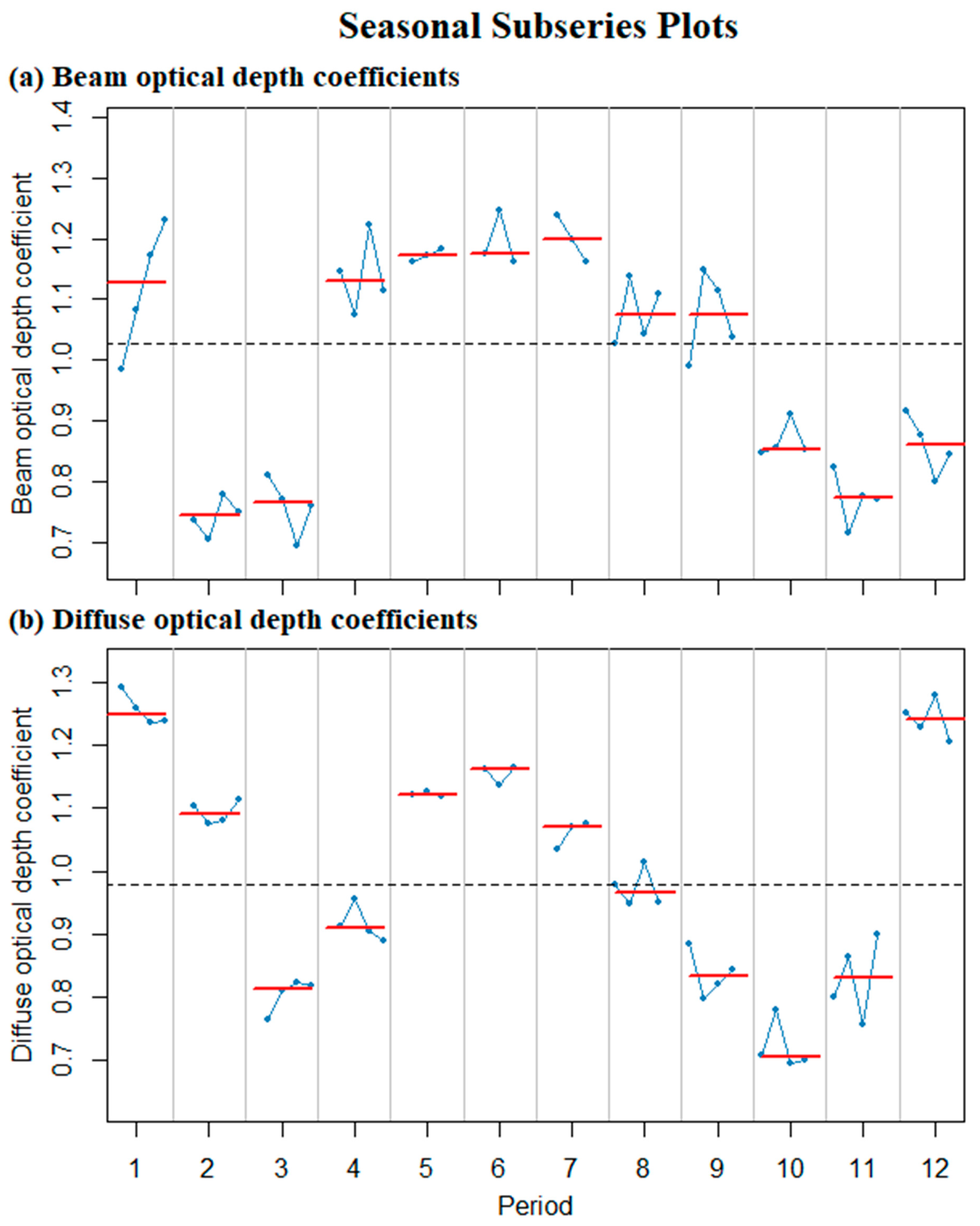
The values of the monthly CSBOD and CSDOD coefficients as functions of time can be visualized in the time series plot in Figure 1. The graph shows the existence of seasonality and trends in the CSBOD coefficients of TS. The CSBOD reaches its higher values in June of the year until August (winter season) and decreases to reach its minimum value between February and March with a sudden increase in January (summer season). After this range, the CSBOD increases again to reach its higher value. The CSDOD decreases from its maximum value in January and increases to reach a certain value in March. The CSDOD increases again from March to July, then decreases again to its lower value in October before increasing to its highest value in January. It can be noticed that the CSDOD presents oscillating behavior during the year. In both cases, it is difficult to determine the exact behavior of the CSBOD and CSDOD coefficients.

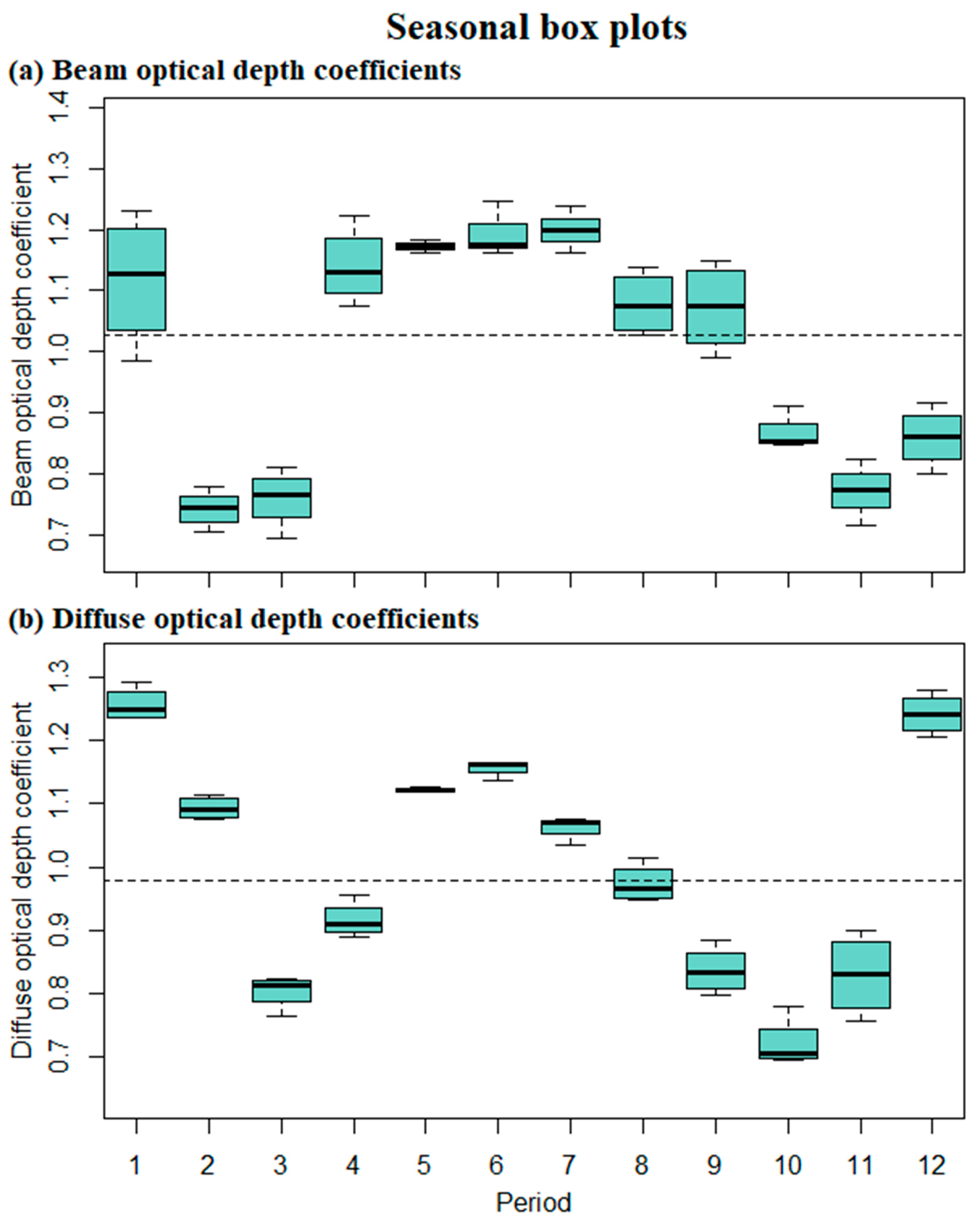
To obtain more details on the data, the decomposition of the time series data in trend, seasonality, and remainder components is performed and seasonal plots analyzed. It shows the existence of seasonal fluctuation occurring without an almost linear trend. Additionally, the random remainder with seasonal strength of 0.9 against a trend strength of 0.2, and seasonal strength of 1 against a trend strength of 0.2, are noted for the CSBOD and CSDOD, respectively. As the seasonal strength is higher compared to the trend strength, a deep analysis of the seasonality is performed using seasonal plot, seasonal subplot, and seasonal boxplot to obtain an explanation of the seasonality strength.

The seasonal plot in Figure 2 shows a seasonal pattern that occurs each year. With observed variances in the years from January to December, it is difficult to obtain more information on the patterns. A clear image of the CSBOD data pattern is obtained with seasonal subplots and seasonal boxplots in Figure 3 and Figure 4, respectively.

The horizontal lines in Figure 3 represent the average CSBOD and CSDOD values grouped by month. A sudden fall of the CSBOD coefficient to its lower value in February from January is noted. From March, the CSBOD coefficient increases to reach its maximum in July. After July, a regressive decrease in the CSBOD can be observed, followed by a new increase from November to January. The same behavior can also be observed the CSDOD that decreases from its maximum in January to a low value in March and increases to a high value in June. From June, the CSDOD decreases to reach its lower value in October, then increases again to its higher value in January.

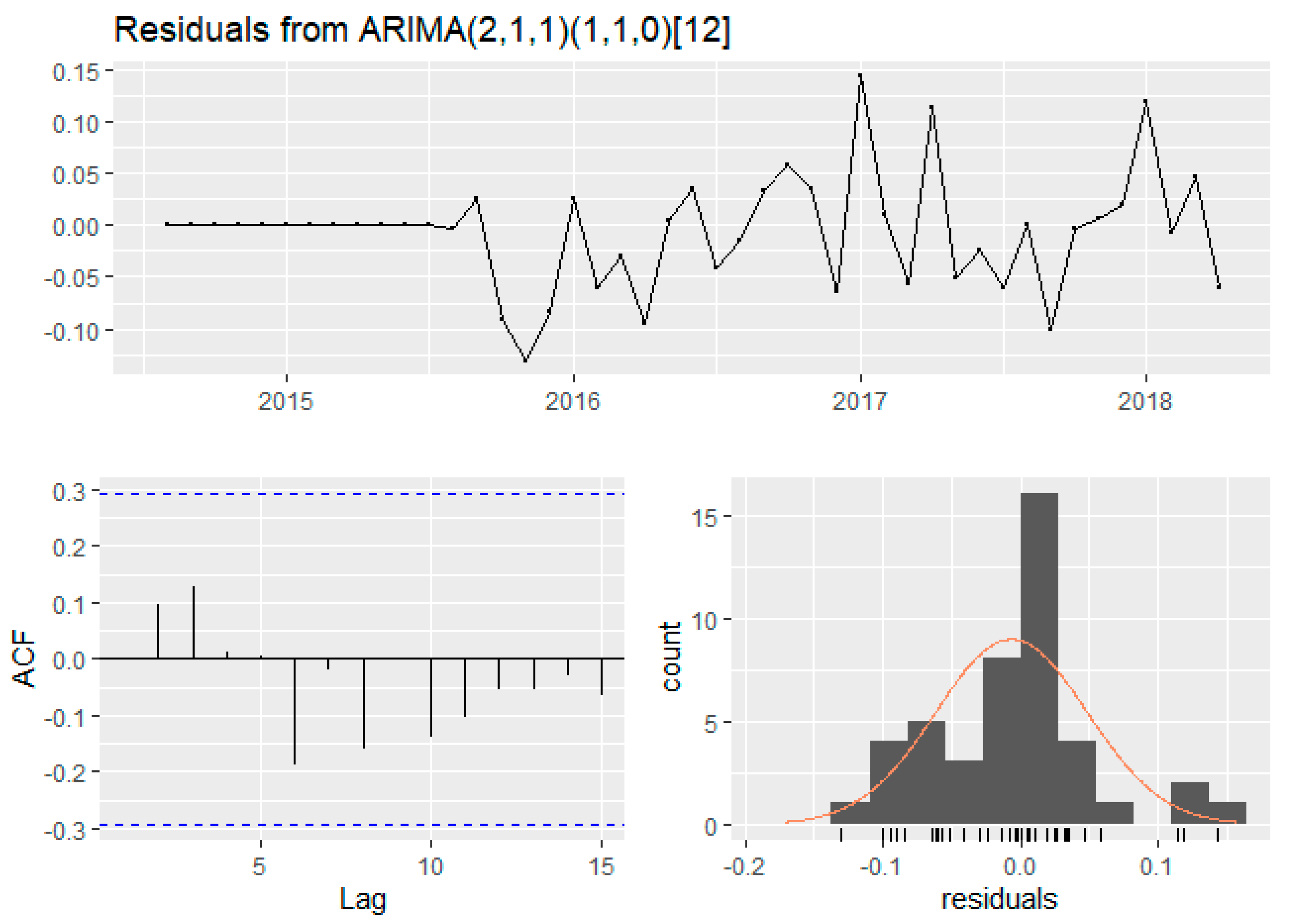
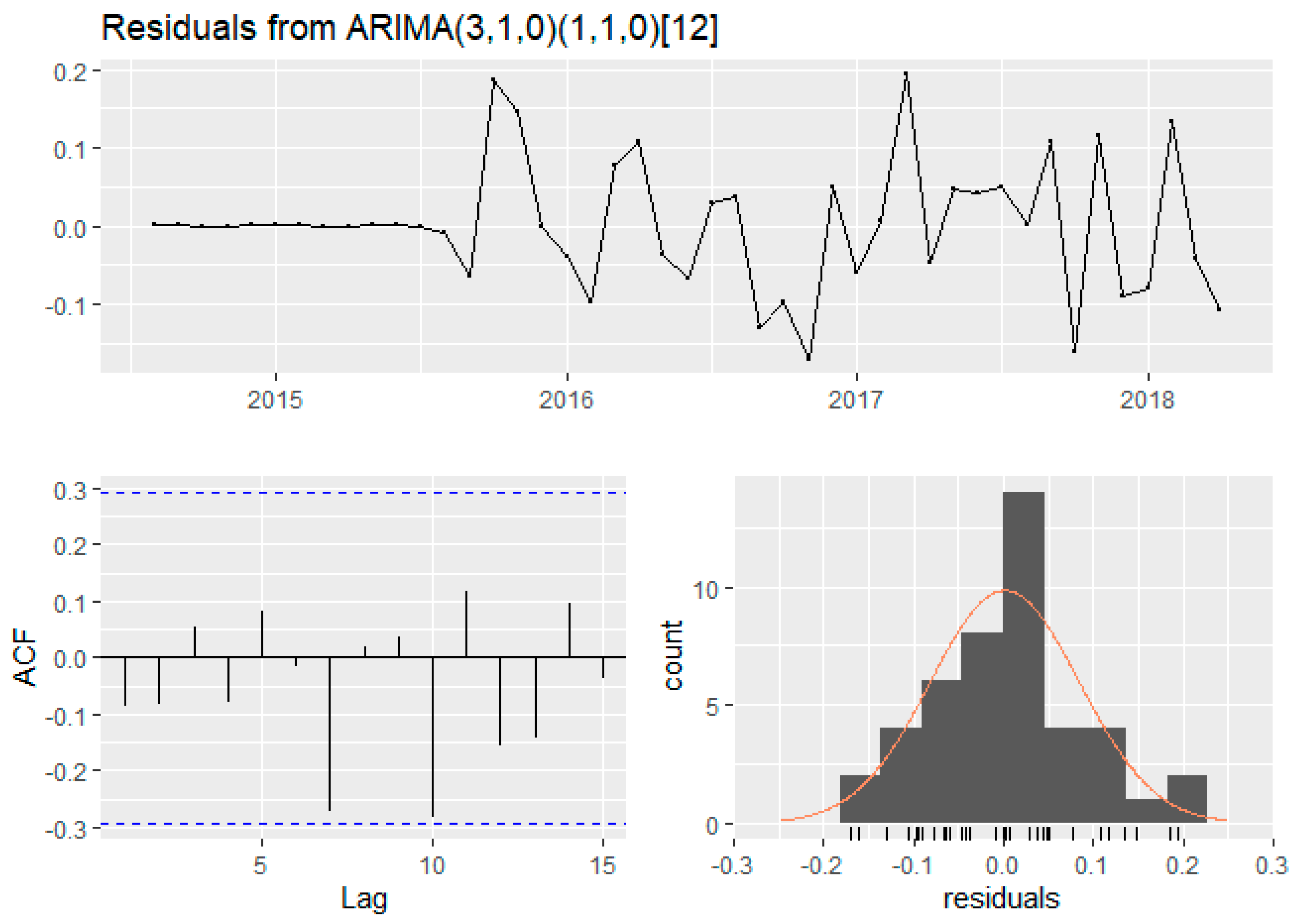
From the seasonal box plots in Figure 4, the data are largely sprayed in January and September for the CSBOD, and November for the CSDOD. A small variability in the coefficient is observed in May for both the CSBOD and CSDOD. Based on the Ljung–Box test and ACF plot of the model residuals in Figure 5 and Figure 6, it can be concluded the ARIMA models are appropriate for these data since their residuals present white noise behaviors and are uncorrelated against each other.

To obtain the ARIMA models of the CSBOD and CSDOD for Durban, different ARIMA (p,d,q) (P,D,Q) [h] were compared and the best of them were selected. The selected ARIMA model was then compared to the Naive model and the ETS (M,N,M) model. The results of the Ljung–Box test are presented in

Table 1. Ljung–Box test results for beam and diffuse optical depths.

Statistic Parameters	Beam Optical Depth			Diffuse Optical Depth
	Naive Method	ETS Model	ARIMA Model	Naive Method	ETS Model	ARIMA Model
Q	9.6967	14.684	4.7057	12.665	28.608	5.7502
df	9	3	5	9	3	5
p-value	0.3756	0.0021	0.4528	0.1784	2.7 × 10−6	0.3313
Model df	0	14	4	0	14	4
Total lags used	9	17	9	9	17	9

, while the statistical analysis for different models of the beam and diffuse optical depths is presented in

Table 2. Statistical analysis for the different models of the beam and diffuse optical depths.

Test	Beam Optical Depth			Diffuse Optical Depth
	Naive Model	ETS Model	ARIMA Model	Naive Method	ETS	ARIMA Model
MPE	106.40	0.2611	−1.1330	−54.724	−0.1012	−0.0026
MAE	0.0843	0.0383	0.0368	0.1433	0.0605	0.0586
MAPE	166.72	4.2783	4.1807	108.62	2.7253	2.7009
RMSE	0.0981	0.0490	0.0547	0.1859	0.0757	0.0819
MASE	1	0.6155	0.5913	1	0.5726	0.5551

.

With an MAE of 3.68% for the CSBOD and 5.86% for CSDOD, it can be deduced at first glance that the ARIMA (2,1,1) (1,1,0) [12] and ARIMA (3,1,0) (1,1,0) [12] are good models for the CSBOD and CSDOD, respectively. Due to the relative size of the error, which is not always evident, the MAPE can be used for more investigations. The MAPE of the ARIMA is 4.18 for the CSBOD and 2.7 for the CSDOD. These values are smaller compared to the values of other models, as can be observed in Table 2. This makes ARIMA the best model from the three selected models. Since the mean error was previously used in both tests, the impact of big and frequent errors may be downplayed. To adjust for the rare large errors, the RMSE is calculated. From the three models, ETS has lower values of RMSE of 4.9% for the CSBOD and 7.6% for CSDOD that could make it the best model. However, for greater accuracy, further investigations are performed on the MASE. The ARIMA models for the CSBOD and CSDOD have lower values of 0.591 and 0.555, respectively. The values lower than 1 lead to ARIMA (2,1,1) (1,1,0) [12] and ARIMA (3,1,0) (1,1,0) [12] to be selected as the models for the CSBOD and CSDOD, respectively.

4. Application Example

The cooling load calculation is performed for a room situated in MUT’s new engineering building. The room has one facade with a sliding window exposed to the sun. The rest of the facades, being inside the building, are completely isolated. The roof of the building is horizontal and entirely exposed to the sun. The solar radiation on the exposed surface areas of the building is calculated by Equations (1) and (2) based on the ASHREA method [33]. In the calculation, the cooling load component related to the internal heat gain from occupancy, lighting, other appliances, and other equipment is not considered. The characteristic of the room is presented in following

Table 3. Room characteristics.

Component	Area (m2)	Material	Surface Azimuth [0]	Surf. Tilt from Horiz. [0]
Roof	14.00	New sheet metal galvanized roof surface.	−45	0
Wall	4.00	White acrylic paint surface wall.	−45	90
Window	6.00	Single glazing-type 5d6 window system.	−45	90

.

The cooling load related to each surface area of the room is obtained from a calculation of the room heat gain of the solar radiation reaching that surface area using the CSBOD of 0.68073 and the CSDOD of 2.64413. These values of the clear sky optical depths are obtained from the ARIMA models for the hottest day on 21 February, and the cooling load calculation is performed following a step-by-step RTSM, as described by the American Society of Heating [33].

The results from the simulation of the cooling load for the room at MUT’s new building are presented in

Table 4. Simulation results for the cooling load of MUT’s new building room.

Local Std. Hour (Hrs)	Wall and Window Solar Irradiance (W)	Roof Solar Irradiance (W)	Wall Cooling Load (W)	Window Cooling Load (W)	Roof Cooling Load (W)	Total Cooling Load (W)
0	0	0	6.8894	81.8090	11.9367	100.6351
1	0	0	5.9455	64.7724	10.5787	81.2966
2	0	0	5.0594	48.2553	9.3571	62.6718
3	0	0	4.2717	35.7263	8.4919	48.4900
4	0	0	3.6275	28.2710	7.8926	39.7911
5	102.6300	44.0217	3.1146	194.0213	7.3696	204.5055
6	353.8490	160.6268	2.9747	816.7486	8.7377	828.4611
7	412.0918	319.5139	3.8572	1105.1196	14.8966	1123.8734
8	370.0991	478.6413	5.9839	1041.6774	28.1285	1075.7898
9	270.4189	613.8186	8.6754	731.4266	46.2352	786.3372
10	140.5037	708.6097	11.1200	442.3355	65.8183	519.2739
11	298.5987	755.0025	12.8998	596.4177	83.7919	693.1094
12	116.6168	741.0646	14.3917	370.7617	97.0910	482.2444
13	106.8468	675.2933	15.5691	300.0449	104.5589	420.1729
14	93.1774	562.2877	16.0585	259.4217	105.5651	381.0453
15	75.9243	414.8976	16.2188	235.6355	100.6220	352.4763
16	56.0850	252.3353	16.2377	206.5021	89.9904	312.7303
17	35.0694	103.9000	15.9242	173.3563	74.1284	263.4089
18	19.9962	39.7395	15.1109	146.9955	55.7983	217.9047
19	0	0	13.8759	118.2320	39.7908	171.8987
20	0	0	12.3557	103.6728	27.8380	143.8666
21	0	0	10.7259	95.8722	20.1479	126.7460
22	0	0	9.2052	92.1492	15.8262	117.1807
23	0	0	7.9439	87.5994	13.5509	109.0942

.

The total cooling load related to the external heat gain is presented in Figure 7a. It is noticed that the window cooling load has a higher impact on the total cooling load related to solar irradiance. As the heat transfer of a material is inversely proportional to its heat transfer coefficient, the window cooling load can be reduced by opting for a different type of window with a low heat transfer coefficient. This reduces the amount of heat gain by the room through the windows based on the material’s thermal resistance, the double-glazed window design, or the combination of both. The window cooling load is followed by a small quantity of roof cooling load and an almost non-existing wall cooling load. It is also noticed from Figure 7b,c that the beam component of the solar irradiance significantly contributes to the total cooling load, while the low contribution of the diffuse and ground reflected irradiances is observed for all the room surface areas. The beam component of solar irradiance is always higher than the diffuse component, which is the case from the obtained results. This confirms the validity of the obtained results. Furthermore, the contribution of the ground reflected irradiance is zero for the roof. This component of solar irradiance is generally a small amount of irradiance, and it is entirely absorbed by the wall and window before reaching the roof of the building. The maximum cooling load of 1124 W is reached for the room at 7h:00. This is the time at which the wall and the window receive the maximum amount of solar irradiance of 412 W. After 7h:00, the solar irradiance reaching the wall starts to decrease with an increase in the solar zenith angle.

5. Conclusions

The availability of the measured clear sky global horizontal irradiance and clear sky diffuse horizontal irradiance data from SURAN LAB made it possible to determine the clear sky beam optical depth (CSBOD) and the clear sky diffuse optical depth (CSDOD) for the Umlazi area. Additionally, from the obtained solar data, the Autoregressive Integrated Moving Average (ARIMA) models for both the CSBOD and CSDOD were developed. The proposed models were validated by comparison to the Error, Trend, Seasonality (ETS) and Naive models for accuracy. The RMSE for the CSBOD and CSDOD were 5.47% and 8.19%, respectively. The obtained MAPE was 4.18 for the CSBOD and 2.7 for CSDOD. The results obtained for the ARIMA models are in good agreement with the ETS models for both the CSBOD and CSDOD, in comparison to the Naive models, MASE < 1. Using the obtained values of 0.68073 and 2.64413 for the CSBOD and CSDOD, the solar irradiance heat gain on the wall, window, and roof were obtained for different facades of the room exposed to the sun. The obtained solar irradiances allowed for the calculation of the room cooling load of 1124 W.

The obtained CSBOD and CSDOD models can be used in the calculation and forecast of the beam horizontal and direct normal irradiance for a specific surface, knowing the solar zenith angle. This enables the accurate calculation of the thermal cooling load related to the solar radiation gain for HVAC systems designed for buildings in the Umlazi area, and improves the control of these systems by knowing the forecasted thermal or cooling load.

References

1. Liang, C.; Li, X.; Melikov, A.K.; Shao, X.L.; Li, B. A quantitative relationship between heat gain and local cooling load in a general non-uniform indoor environment. Energy 2019, 182, 412–423. [Google Scholar] [CrossRef]
2. Chenari, B.; Carrilho, J.D.; da Silva, M.G. Towards sustainable, energy-efficient and healthy ventilation strategies in buildings: A review. Renew. Sustain. Energy Rev. 2016, 59, 1426–1447. [Google Scholar] [CrossRef]
3. Toparlar, Y.; Blocken, B.; Maiheu, B. Impact of urban microclimate on summertime building cooling demand: A parametric analysis for Antwerp, Belgium. Appl. Energy 2018, 228, 852–872. [Google Scholar] [CrossRef]
4. Ürge-Vorsatz, D.; Cabeza, L.F.; Serrano, S.; Barreneche, C.; Petrichenko, K. Heating and cooling energy trends and drivers in buildings. Renew. Sustain. Energy Rev. 2015, 41, 85–98. [Google Scholar] [CrossRef] [Green Version]
5. Vakiloroaya, V.; Samali, B.; Fakhar, A. A review of different strategies for HVAC energy saving. Energy Convers. Manag. 2014, 77, 738–754. [Google Scholar] [CrossRef]
6. Kabanshi, A.; Ameen, A.; Hayati, A. Cooling energy simulation and analysis of an intermittent ventilation strategy under different climates. Energy 2018, 156, 84–94. [Google Scholar] [CrossRef] [Green Version]
7. Jing, R.; Wang, M.; Zhang, R.; Li, N.; Zhao, Y. A study on energy performance of 30 commercial office buildings in Hong Kong. Energy Build. 2017, 144, 117–128. [Google Scholar] [CrossRef]
8. Yan, D.; Zhe, T.; Yong, W.; Zhu, N. Achievements and suggestions of heat metering and energy efficiency retrofit for existing residential buildings in northern heating regions of China. Energy Policy 2011, 39, 4675–4682. [Google Scholar] [CrossRef]
9. Zhou, X.; Yan, D.; Hong, T.; Ren, X. Data analysis and stochastic modelling of lighting energy use in large office buildings in China. Energy Build. 2015, 86, 275–287. [Google Scholar] [CrossRef] [Green Version]
10. Energy Technology Perspectives 2016; International Energy Agency (IEA): Paris, France, 2016; Available online: https://www.iea.org/reports/cooling (accessed on 28 February 2022).
11. Kapetanakis, D.S.; Mangina, E.; Finn, D.P. Input variable selection for thermal load predictive models of commercial buildings. Energy Build. 2017, 137, 13–26. [Google Scholar] [CrossRef]
12. Li, X.W.; Wen, J. Review of building energy modeling for control and operation. Renew. Sustain. Energy Rev. 2014, 37, 517–537. [Google Scholar] [CrossRef]
13. Pérez-Lombard, L.; Ortiz, J.; Pout, C. A review on buildings energy consumption information. Energy Build. 2008, 40, 394–398. [Google Scholar] [CrossRef]
14. Niu, J.; Tian, Z.; Lu, Y.; Zhao, H.; Lan, B. A robust optimization model for designing the building cooling source under cooling load uncertainty. Appl. Energy 2019, 241, 390–403. [Google Scholar] [CrossRef]
15. Xiang-Li, L.; Zhi-Yong, R.; Lin, D. An investigation on life-cycle energy consumption and carbon emissions of building space heating and cooling systems. Renew. Energy 2015, 84, 124–129. [Google Scholar] [CrossRef]
16. Macas, M.; Moretti, F.; Fonti, A.; Giantomassi, A.; Comodi, G.; Annunziato, M.; Pizzuti, S.; Capra, A. The role of data sample size and dimensionality in neural network based forecasting of building heating related variables. Energy Build. 2016, 111, 299–310. [Google Scholar] [CrossRef]
17. Zainal, O.A.; Yumrutas, R. Validation of periodic solution for computing CLTD (cooling load temperature difference) values for building walls and flat roofs. Energy 2015, 82, 758–768. [Google Scholar] [CrossRef]
18. Sarwar, R.; Cho, H.; Cox, S.J.; Mago, P.J.; Luck, R. Field validation study of a time and temperature indexed autoregressive with exogenous (ARX) model for building thermal load prediction. Energy 2017, 119, 483–496. [Google Scholar] [CrossRef]
19. Ding, Y.; Zhang, Q.; Yuan, T. Research on short-term and ultra-short-term cooling load prediction models for office buildings. Energy Build. 2017, 154, 254–267. [Google Scholar] [CrossRef]
20. Li, X.; Liu, K.; Tian, J. Variability, predictability, and uncertainty in global aerosols inferred from gap-filled satellite observations and an econometric modeling approach. Remote Sens. Environ. 2021, 261, 112501. [Google Scholar] [CrossRef]
21. Yu, F.; Yue, Q.; Yunianta, A.; Aljahdali, H.M.A. A novel hybrid deep correction approach for electrical load demand prediction. Sustain. Cities Soc. 2021, 74, 103161. [Google Scholar] [CrossRef]
22. Dubey, A.K.; Kumar, A.; García-Díaz, V.; Sharma, A.; Kanhaiya, K.S.S. Study and analysis of SARIMA and LSTM in forecasting time series data. Sustain. Energy Technol. Assess. 2021, 47, 101474. [Google Scholar]
23. Lee, D.-S.; Jo, J.-H.; Koo, S.-H.; Lee, B. Development of Climate Indices Using Local Weather Data for Shading Design. Sustainability 2015, 7, 1884–1899. [Google Scholar] [CrossRef] [Green Version]
24. Jannat, N.; Hussien, A.; Abdullah, B.M.; Cotgrave, A.J. A Comparative Simulation Study of the Thermal Performances of the Building Envelope Wall Materials in the Tropics. Sustainability 2020, 12, 4892. [Google Scholar] [CrossRef]
25. Gou, S.; Nik, V.M.; Scartezzini, J.-L.; Zhao, Q.; Li, Z. Passive design optimization of newly-built residential buildings in Shanghai for improving indoor thermal comfort while reducing building energy demand. Energy Build. 2018, 169, 484–506. [Google Scholar] [CrossRef]
26. Konstantinou, T.; Ignjatović, Ć.N.; Zbašnik-Senegačnik, M. Energy: Resources and Building Performance; TU Delft Open: Delft, The Netherlands, 2018. [Google Scholar]
27. Badea, N. Design for Micro-Combined Cooling, Heating and Power Systems. In Stirling Engines and Renewable Power Systems, 1st ed.; Springer: London, UK, 2015. [Google Scholar]
28. Mao, C.; Baltazar, J.-C.; Haberl, J.S. Literature review of building peak cooling load methods in the United States. Sci. Technol. Built Environ. 2018, 24, 228–237. [Google Scholar] [CrossRef]
29. Lv, L.; Huang, C.; Li, L.; Chen, J. Experimental study on calculation method of the radiant time factors. Renew. Energy 2015, 73, 28–35. [Google Scholar] [CrossRef]
30. Spitler, J.D.; Fisher, D.E.; Pedersen, C.O. The radiant time series cooling load calculation procedure. ASHRAE Trans. 1997, 103, 503–515. [Google Scholar]
31. Spitler, J.D.; Fisher, D.E. On the Relationship between the Radiant Time Series and Transfer Function Methods for Design Cooling Load Calculations. HVAC&R Res. 1999, 5, 123–136. [Google Scholar]
32. McQuiston, F.C.; Parker, J.D.; Spitler, J.D. Heating Ventilating and Air Conditioning Analysis and Design, 6th ed.; John Wiley & Sons Inc.: San Francisco, CA, USA, 2005. [Google Scholar]
33. 2017 ASHRAE Handbook—Fundamentals (SI); American Society of Heating, Refrigerating and Air-Conditioning Engineers: Atlanta, GA, USA, 2017.
34. Optical Depth. Wikipedia, The Free Encyclopedia. 2020. Available online: https://en.wikipedia.org/wiki/Optical_depth (accessed on 28 February 2022).
35. Kim, S.-W.; Choi, I.-J.; Yoon, S.-C. A multi-year analysis of clear-sky aerosol optical properties and direct radiative forcing at Gosan. Atmos. Res. 2010, 95, 279–287. [Google Scholar] [CrossRef]
36. Tang, W.; Yang, K.; Qin, J.; Niu, X.; Lin, C.; Jing, X. A revisit to decadal change of aerosol optical depth and its impacts on global radiation over China. Atmos. Environ. 2017, 150, 106–115. [Google Scholar] [CrossRef]
37. Kudish, A.I.; Evseev, E.G. UVB irradiance and atmospheric optical depth at the Dead Sea basin, Israel: Measurements and modeling. Renew. Energy 2012, 48, 344–349. [Google Scholar] [CrossRef]
38. Serrano, M.A.; Boscà, J.V.; Cañada, J. The determination of a band factor to express irradiance of UV and PAR wavelength ranges in a clean and dry atmosphere at Valencia, Spain. Int. J. Ambient Energy 2008, 29, 171–180. [Google Scholar] [CrossRef]
39. Kasten, F.; Young, A.T. Revised optical air mass tables and approximation formula. Appl. Opt. 1989, 28, 4735–4738. [Google Scholar] [CrossRef] [PubMed]
40. Iqbal, M. An Introduction To Solar Radiation; Academic Press: Toronto, ON, Canada, 1983. [Google Scholar]
41. Elsaraiti, M.; Merabet, A. A Comparative Analysis of the ARIMA and LSTM Predictive Models and Their Effectiveness for Predicting Wind Speed. Energies 2021, 14, 6782. [Google Scholar] [CrossRef]
42. Bento, P.M.R.; Pombo, J.Á.N.; Calado, M.d.R.; Mariano, S.J.P.S. Stacking Ensemble Methodology Using Deep Learning and ARIMA Models for Short-Term Load Forecasting. Energies 2021, 14, 7378. [Google Scholar] [CrossRef]
43. Liu, X.; Lin, Z.; Feng, Z. Short-term offshore wind speed forecast by seasonal ARIMA—A comparison against GRU and LSTM. Energy 2021, 227, 120492. [Google Scholar] [CrossRef]
44. Bashir, T.; Haoyong, C.; Tahir, M.F.; Liqiang, Z. Short term electricity load forecasting using hybrid prophet-LSTM model optimized by BPNN. Energy Rep. 2022, 8, 1678–1686. [Google Scholar] [CrossRef]
45. Hassan, J. ARIMA and regression models for prediction of daily and monthly clearness index. Renew. Energy 2014, 68, 421–427. [Google Scholar] [CrossRef]
46. Ghoneim, A.A.; Kadad, I.M.; Altouq, M.S. Statistical analysis of solar UVB and global radiation in Kuwait. Energy 2013, 60, 23–34. [Google Scholar] [CrossRef]
47. Mutombo, N.M.-A.; Mukuna, J.G.M.; Zawilska, E. Preliminary Analysis of Ground-Based Measured Solar Data from Sauran STA Station at Umlazi, South Africa. Int. J. Mech. Eng. Technol. 2019, 10, 104–113. [Google Scholar]
48. Huang, J.; Korolkiewicz, M.; Agrawal, M.; Boland, J. Forecasting solar radiation on an hourly time scale using a Coupled Auto Regressive and Dynamical System (CARDS) model. Solar Energy 2013, 87, 136–149. [Google Scholar] [CrossRef]
49. Hassan, A.; Hejase, N.; Assi, A.H. Time-series regression model for prediction of mean daily global solar radiation in Al-Ain, UAE. Int. Sch. Res. Not. 2012, 2012, 1–11. [Google Scholar]
50. Sulaiman, M.Y.; Oo, W.M.H.; Wahab, M.A.B.D.; Sulaiman, Z.A. Analysis of residuals in daily solar radiation time series. Renew. Energy 1997, 11, 97–105. [Google Scholar] [CrossRef] [Green Version]
51. Zaharim, A.; Razali, A.M.; Gim, T.P.; Sopian, K. Time series analysis of solar radiation data in the tropics. Eur. J. Sci. Res. 2009, 25, 672–678. [Google Scholar]
Figure 1. Clear sky optical depth coefficient time series plots. (a) BOD coefficients from August 2014 to April 2018. (b) Diffuse optical depth coefficients from August 2014 to April 2018.
Sustainability 14 03662 g001
Figure 2. Clear sky optical depth coefficient time series seasonal plots. (a) Beam optical depth coefficients. (b) Diffuse optical depth coefficients.
Sustainability 14 03662 g002
Figure 3. Clear sky optical depth coefficient time series seasonal sub-series plots. (a) Beam optical depth coefficients. (b) Diffuse optical depth coefficients.
Sustainability 14 03662 g003
Figure 4. Clear sky optical depth coefficient time series seasonal boxplots. (a) Beam optical depth coefficients. (b) Diffuse optical depth coefficients.
Sustainability 14 03662 g004
Figure 5. Clear sky beam optical depth coefficients time series residual check on the ARIMA model.
Sustainability 14 03662 g005
Figure 6. Clear sky diffuse optical depth coefficients time series residual check on the ARIMA model.
Sustainability 14 03662 g006
Figure 7. Cooling load and related solar irradiance for different surface areas of MUT’s new room. (a) Solar cooling load. (b) Wall and window solar irradiance. (c) Roof solar irradiance.
Sustainability 14 03662 g007