1. Introduction
There is a high interest in the use of photovoltaic (PV) energy since it is a non-pollutant and an environmental-friendly alternative. Nevertheless, besides its advantages, the performance of the PV installations depends on the weather conditions, which can be dynamic over time. Shading caused by trees, buildings, or passing clouds can be projected on the PV panels, causing drops in the generated power [
1,
2].
To mitigate the effect of total or partial shading, researchers developed several strategies as the use of the bypass diode, which gives an alternative path to the current so the PV panels do not consume any power. However, this solution introduces multi-peaks in the current vs. voltage (I–V) curves of the PV array due to the diode activation [
3,
4].
Another strategy is the maximum power point tracking (MPPT), which implies using algorithms such as P&O, fuzzy logic, and incremental conductance, to seek the optimum operation point known as maximum power point (MPP) of the PV array [
5,
6].
One of the most common practices to reduce the effect of partial shading is reconfiguration. This process involves changing the physical or electrical connections of the panels in the PV array, using a switching matrix based on relays as in [
7,
8,
9].
The different connections between the panels are known as configurations, which can be regular configurations following a defined pattern such as total-cross-tied (TCT), series-parallel (SP), bridge linked (BL), and honey comb (HC). Similarly, modern configurations such as SuDoKu puzzle and Magic Square have their own previously established pattern [
10,
11,
12]. Instead, irregular configurations do not follow any pattern.
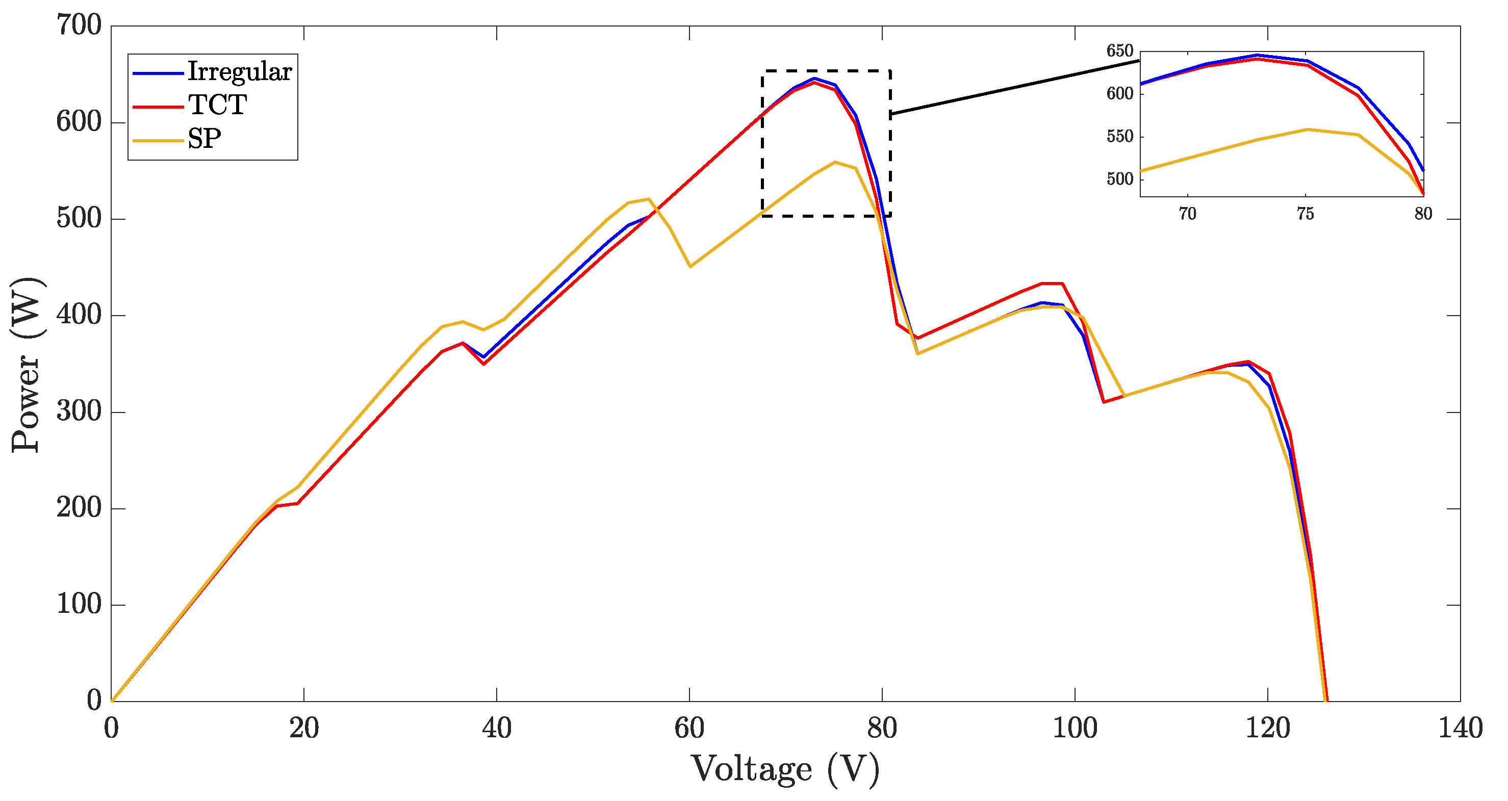
Depending on the shading pattern or the environmental conditions on the PV array, a given amount of power can be obtained with each configuration. The goal of the reconfiguration process is to find the configuration which can extract the highest amount of energy. An example is presented in
Figure 1, where a TCT configuration is compared with an SP and an irregular one. TCT obtained 641.5124 W, SP delivered 559.1170 W, and the irregular one delivered 646.0916 W. This example shows that the irregular configuration, in this particular example, provides the highest power.
One of the main challenges in the reconfiguration procedure is finding the correct combination in minimal time; this problem can be addressed by considering reconfiguration as an optimization problem.
The use of metaheuristic techniques in the reconfiguration process aims at the deployment of the optimum configuration for the working conditions of the PV array before the weather conditions change. In this matter, metaheuristic techniques such as PSO [
13], marine predator [
14], GOA [
15], and GA [
16] have been proposed in contrast with techniques based on brute force or analytical methods, which might require longer execution times to perform the reconfiguration of the PV array.
There also exists the drawback of the complexity of mathematical models used to solve the resulting equations of the PV array analysis. To address this problem, techniques such as Newton–Raphson, Lambert-W, or Levenberg–Marquardt have been adopted; those techniques can lead to complex procedures to calculate the current and voltage of a PV array under a particular irradiance and temperature condition [
17,
18,
19]. This problem has been simplified assuming one single configuration. Some authors [
16,
20] have faced the reconfiguration problem with GAs considering the TCT configuration as a static array, changing the physical position of the PV panels to disperse the shadow without changing its connection. Other authors use the SP configuration [
21,
22] since it can simplify the equation system by not having a direct parallel connection between the PV strings. Nevertheless, not considering all the configurations in the PV array decreases the versatility of the procedures, avoiding an analysis of the energy impact problem, which might lead to energy losses due to the implementation of improper configurations [
23,
24].
Considering the previous mitigation strategies, the problem of the energy impact generated by partial shading has been a subject of study since it is one of the main sources of power losses, both for static shadows such as those given by buildings, as well as dynamic shadows such as those caused by clouds [
25,
26]. These studies often use metrics such as fill factor, percentage of power loss, and performance ratio [
27,
28], which enable to quantify the power loss due to shading or mismatching between PV panels characteristics.
With a study of the impact of the configurations in PV arrays under different solar irradiation conditions, it is possible to have an idea of the energy losses that may occur at the PV array site, especially if there is information on the shading present in the area. To address reconfiguration as an optimization problem, by taking into account the quantification of the energy impact of the partial shading conditions, this paper proposes a reconfiguration procedure based on a GA to find the configuration with the maximum power. The performance of the GA is then compared with a traditional brute force algorithm to verify that the proposed solution overcomes the problem of long execution times. To calculate the maximum power, the work presented in [
29] is used. In this way, the current and voltage of the possible configurations of any PV array are calculated, which consider the modification of the electrical connection between the panels (i.e., dynamic reconfiguration) under partial shading conditions.
Moreover, this paper analyzes the impact of different patterns of dynamic shading on the most common configurations, which are contrasted with those obtained by the GA using metrics such as FF, to quantify the percentage of power lost due to weather conditions and the non-deployment of the appropriate configuration.
This paper is organized as follows:
Section 2 describes the highlights of the modeling procedure used to calculate the current and voltage of the PV arrays, as well as the explanations of the concepts of the proposed technique based on the genetic algorithm.
Section 3 presents the simulation results for the tests performed. Finally, the conclusions are presented in
Section 4.
3. Results
The cases used to evaluate the performance of the proposed methodology were carried out at simulation level, using different irradiance profiles. Those tests consider 18 JS65 Yingli panels forming a 6 × 3 PV array, and the simulations were executed using MATLAB/Simulink software on a computer with an Intel(R) Xeon(R)CPU
[email protected] GHz 2.90 GHz (dual processor), 48 GB RAM, and Windows 10 PRO. The metrics adopted for comparison between the GA reconfiguration results and other common configurations such as SP are the execution time and maximum power. Moreover, this section presents an application case with several sizes of PV arrays, under a dynamic shading condition, to compare the proposed technique with the BF approach in terms of execution time.
Table 2 shows the first case corresponding to the reported mismatching matrix, along with the configurations found by the BF approach and the proposed GA. As
Table 3 shows, the maximum power obtained for both algorithms is the same. Nevertheless, the proposed GA is 98.86% faster than the BF.
Figure 4 illustrates the power vs. voltage (P–V) curves of the GA result along with the irregular configuration given in
Table 2 and a SP configuration. This comparison exhibits a power loss of 37.631 W between the SP, which is a commonly-used configuration, and the configuration given by the GA, while the irregular configuration exhibits a loss of 19.132 W.
Table 4 and
Table 5 report the second case. As it was stated for the first case, the maximum power delivered is the same for both algorithms, but the proposed GA provides an improvement of 99.913% in the execution time.
Figure 5 reports the P–V curves corresponding to the mismatching profile of
Table 4. For this case, the SP configuration has a loss of 20.712 W, while the irregular configuration presents a loss of 15.293 W compared with the maximum power given by the proposed GA.
Moreover, this work also considers the fill factor (FF) [
6] for performance measurement: Equation (
10) is for full illumination conditions and Equation (
11) is for partial shading conditions, where GMPP stands for global MPP:
Table 6 shows the percentage of power loss for the shading scenarios previously described. First, it is necessary to calculate the FF for the full illumination condition, i.e., without any shade present, to consider that value as a base for power loss calculation. This result is obtained using the datasheet data of the JS65 Yingli and the size of the PV array, which has a maximum delivered power of 1.5417 kW. Then, using Equation (
10), the FF of the PV array is calculated as
.
As
Table 6 shows, the SP configuration provides the highest percentage of power losses for both mismatching profiles; therefore, the configuration found by the proposed GA provides a better performance during the partial shading conditions under analysis: the GA shows an improvement of 7.493% for mismatching matrix 1 and 3.855% for mismatching matrix 2.
Table 7 presents some reconfiguration approaches reported in the literature, where most of them require current and voltage measures. On the other hand, those approaches consider regular configurations (SP, TCT, HC, BL), which is a remarkable disadvantage with respect to the procedure proposed in this paper which is capable of also analyzing irregular configurations. Therefore, the proposed approach can deliver a more detailed analysis of a PV array, thus improving the possibility to achieve a higher power production.
Analysis of Shading Impact in PV Power Generation
Concerning the results given by the proposed GA in terms of execution time, such a technique can be recommended for both large-scale PV reconfiguration and as a technique for energy impact evaluation considering dynamic shading conditions. In that way, this section presents an analysis of the impact of different shading patterns on PV arrays with different sizes.
Figure 6 and
Figure 7 show two patterns of dynamic shadows during a day, which are used to simulate the array power production with the proposed GA. Such a performance is contrasted with the results obtained with other known configurations such as SP, TCT, and an irregular one.
Figure 8 shows a summary of the results obtained from those simulations. In the case of the diagonal pattern, the GA obtained the optimum configuration for maximizing the generated power with an irregular configuration. Comparing the power calculated by GA (i.e., irregular 2) with an SP configuration, there exists a power loss of 314 W daily, while for the irregular configuration, 1 is a power loss of 100 W daily, approximately. In the case of rectangular patterns, the configuration found (i.e., SP) was also the optimum along with an irregular configuration and TCT.
According to this information, it is necessary to highlight that not adopting shading mitigation techniques might lead to a reduction in the lifetime of the PV array, economic losses, and unbalance in the loads due to the power losses produced by the shading profiles of the installation zone.
Figure 9 reports that the GA was 963% faster than the BF for the evaluation of the diagonal pattern, and the GA was 1542% faster than the BF for the rectangular pattern. Considering the execution time, the proposed procedure requires a much shorter processing time. Therefore, having a daily shading profile already established, the optimal configuration can be deployed faster to minimize the power losses.
Finally,
Figure 10 compares the processing time required by BF and GA algorithms to reach the optimal solution for a different number of modules, between 8 and 108, which corresponds to a PV array where the rows are increasing from 2 × 4 to 27 × 4. The black dots highlight the execution time of both algorithms for 20, 40, 60, 80, and 100 panels. For the BF approach, an interpolation of the execution time was made from 24 panels to 60 panels. For 24 panels, the execution time of the BF is about 14.75 h (i.e., 53,100 s), while GA only requires 0.033 ms for the same number of panels. Therefore, the GA solution allows to simulate a higher number of panels. Similarly, for 108 panels (27 × 4 array), the execution time of the GA was only 0.074 ms.
4. Conclusions
This paper describes a procedure based on a GA as a reconfiguration and energy impact analysis tool, which evaluates the power levels of different PV array sizes and configurations under distinct environmental conditions. For comparison purposes, a BF approach previously published was also implemented. The proposed GA approach reduces, significantly, the computational burden for PV array simulations. Moreover, for large PV arrays, the BF approach supposes an exponential increase in the execution time due to the calculation of every possible configuration for maximizing the generated power. For a reconfiguration process, according to the information of
Figure 10, this is very impractical in contrast with the proposed procedure based on a GA.
Considering the execution time, this GA-based tool can work under changing environmental conditions, such as dynamic shadows, to calculate the appropriate configuration in the PV array installation place.
In addition, as it was presented in this work, a proper reconfiguration process implies lower power losses, also increasing the PV array lifetime. Disregarding the suitable configuration of a PV array might lead to possible faults in the loads and a loss of energy over time, which might affect the return of investment calculation.


 ,
, 


