Spatial Analysis of Inequality in Thailand: Applications of Satellite Data and Spatial Statistics/Econometrics

Abstract

To formulate and monitor the progress of development policies, acquiring data with sufficient spatiotemporal details is inevitable. With the increasing availability of open remote-sensing data and open-source software packages, this research suggested the novelty integration of satellite data and spatial analytical methods, enabling a timely and costless framework for assessing the nationwide socioeconomic condition. Specifically, the spatial statistical and spatial econometrical methods were applied to geospatial data to identify the clustering patterns and the localized associations of inequality in Thailand. The spatial statistical results showed that Bangkok and its vicinity had been a cluster of high socioeconomic conditions, representing the spatial inequality of development. In addition, results of the spatial econometrical models showed that the satellite-based indicators could identify the socioeconomic condition (with p-value < 0.010 and R-squared ranging between 0.345 and 0.657). Inequality indicators (i.e., Gini, Thiel and Atkinson) were then constructed by using survey-based and satellite-based data, informing that spatial inequality has been slowly declining. These findings recommended the new establishment of polycentric growth poles that offer economic opportunities and reduce spatial inequality. In addition, in accordance with Sustainable Development Goal 10 (reduced inequalities), this analytical framework can be applied to country-specific implications along with the global scale extensions.

1. Introduction

The Thai economy has been continuously evolving, particularly since the implementation of the first national development plan in 1961. The development process has induced the gradual change of social and economic structure, transforming the agricultural-based system into the higher intensity of industrial and service activities. This progress leads to a higher standard of living, as indicated by the continuous higher life expectancy, literacy rate, and average income. During the period 1988–2019, poverty headcount has been substantially declining from 61.41% to 5.04% [1].

Although Thailand’s economic development over the course of six decades has been relatively fruitful, the economic development remains limited and fragmented in geographical dimensions. Development of infrastructure and concentration of economic activity have been largely clustering in Bangkok metropolitan areas, and the rural areas relatively remain at a lower level. In particular, Thailand globally ranked first for the urban primacy index, indicating the largest gap between the size of the largest city and those of the second and third ones [2]. Similarly, some studies documented the similar issue of Thailand’s monocentric growth pole, a spatial concentration of economic growth in Bangkok metropolis and vicinity [3,4]. A study that applied quantitative methods to the official industrial census also confirmed the long-term persistence of this disproportionate spatial pattern of industrial growth with statistically significant indicators [5]. This spatial inequality can impede future economic growth due to the lack of opportunity to fully utilize the regional potentials and initiate alternative growth poles. Equally important, this disproportionate development can simultaneously incur environmental and social problems. In addition, this problem is internationally recognized and studied on a global scale and at country level, motivated by development of empirical findings and data-driven analytical methods [6,7,8,9].

On the basis of these facts, understanding Thailand’s spatial inequality is crucial for future policy formulations and development sustainability. Hence, this study aims to quantitatively investigate the spatial inequality in Thailand by incorporating survey-based data, satellite imageries, and spatial analysis techniques. In particular, two official socioeconomic datasets produced by National Statistical Office (NSO), namely, Socio-Economic Survey (SES) and Thailand Poverty Map, are the survey-based socioeconomic indicators in this analysis. These data were analyzed in conjunction with a set of geospatial data obtained from Google Earth Engine, including satellite-detected nighttime light (NTL), normalized vegetation difference index (NDVI), land surface temperature (LST), and rainfall statistics. The spatial statistical and spatial econometrical methods were applied to these data to quantify the degree of spatial inequality and examine the spatial associations between survey-based indicators and satellite data. The results obtained from spatial statistical techniques unveil the historical and spatial characteristics of disproportionate growth in Thailand. The spatial econometrical method (i.e., spatial regression) suggests the satellite-based indicator that can represent the socioeconomic condition, enabling the extensive applications of timely monitoring the spatial inequality and recommending the policy for rebalancing and sustaining the future development.

The structure of this paper is organized as follows. The second section reviews related publications. The third part elaborates the technical foundations of research methods. The fourth section discusses the results. The fifth section concludes the main contributions of this study.

2. Literature Review

Inequality has been recognized as one of the main socioeconomic problems. In particular, the global datasets indicated the worsening trends in many countries, leading to serious concerns among researchers and policymakers [10,11,12]. Simultaneously, geospatial data have been continuously developing to support monitoring the situation and formulating policy [13]. The increasing availability of multi-source data and computational methods enables the extensive development of applications to examine the geographical features of poverty and inequality in many countries [14,15,16,17,18].

The progress of data-driven analyses also facilitates multifaceted studies, for example, the detection of slum locations [19,20]. Also, the inequality indicators derived from satellite data, primarily using the NTL index, were constructed on a global scale, allowing a timely and costless framework for monitoring the global situation of spatial inequality [7,21,22,23]. A similar approach was applied to the country-specific study of poverty and inequality, for example, the cases of African countries [24,25], China [9,26,27], Romania [6], Paraguay [26], Bangladesh [18] and Myanmar [27,28].

With the continuous development of analytical techniques [6,7,22,23] and the internationally rising concerns on inequality [10,11,12,29], this study acknowledged the research gap in the case of Thailand. Therefore, the novelty integration of the open satellite data and the spatial statistical/econometrical methods was introduced. Specifically, this study showed that Google Earth Engine, an open platform, can enable public accessibility and cloud-based geoprocessing of satellite data related to socioeconomic conditions. Likewise, the open-source software packages can facilitate low-cost computational capabilities using geospatial methods. The integrated outcomes would deepen insights on multifaceted associations inducing the geographical clustering pattern of poverty and subsequently empower the investigation of underlying factors, ultimately leading to the formulation of regional development policy.

3. Data

The content in this section provides basic details of the data used in the analysis. Two groups of sources are used with Quantum GIS and GeoDA, open-source spatial analysis software packages. The details of each data group are as follows:

3.1. Data from Surveys

This study used secondary datasets surveyed by the government agency. The survey data used in this study consist of two variables as follows:

3.1.1. Household Income Data

This dataset was obtained from the SES conducted by the NSO of Thailand. These surveys have operated since 1957, selecting randomly from 52,000 households all over the country. The questions of these surveys consist of the details of the entire household, the member’s structure, details of expenses, and the characteristics of the residence. Questions about income are interviewed every two years (with the exception of conducting the annual survey in some years), and random surveys cover households with municipal and nonmunicipal residences. This study used the household income of the period 1992–2017 and then adjusted to average values by each province.

3.1.2. Poverty Data

This variable was obtained from Thailand’s Poverty Map dataset conducted by NSO. This dataset used raw data from the Household SES and Population and Housing Census. It was calculated with the poverty line dataset developed by the National Economic and Social Development Council (NESDC) and Thailand Development Research Institute (TDRI), yielding the proportion of the number of people whose expense is below the poverty line. This study used this dataset of 2013, 2015 and 2017.

3.2. Data from Google Earth Engine

Google Earth Engine is a satellite data service that Google has opened to the public to access geospatial datasets. This platform provides a wide range of data from various sources, allowing users to code, select, calculate, and adjust the data by their specific requirements. The satellite data used in this study consist of four variables as follows:

3.2.1. NTL Data

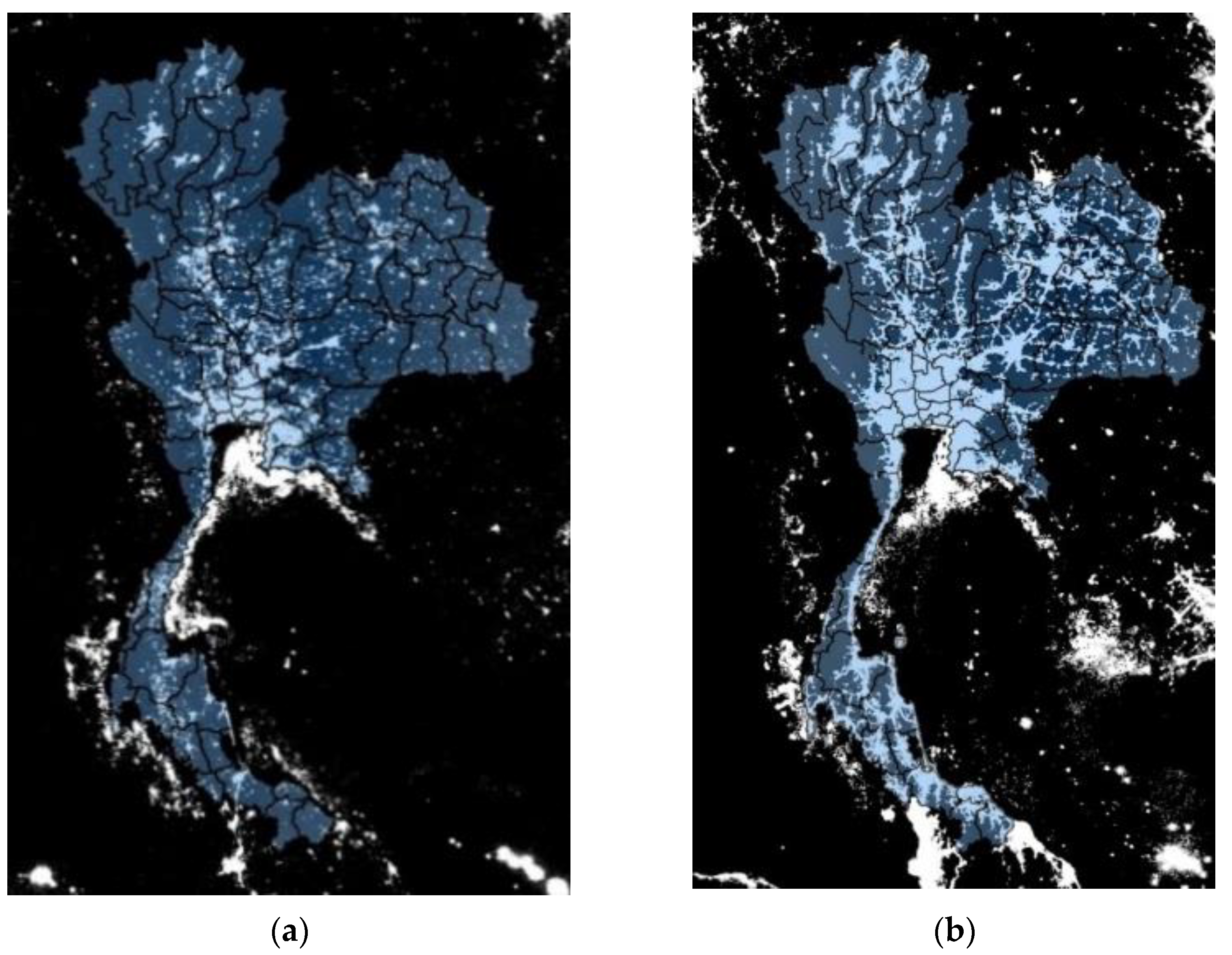
NTL data are satellite imagery of the Earth at night consisting of two datasets. The first is obtained from satellites under the DMSP, which uses a sensor system called OLS. This satellite provided the images from 1992 to 2014. The images obtained resulted from light detection by using image sensors during light ranges visible near-infrared (VNIR) from 8:30 p.m. to 10:00 p.m. for each spot on the Earth’s surface. The National Oceanic and Atmospheric Administration has enhanced some errors of the images, such as moonlight in the upward range, the light from the summer sun with a long daytime, the disturbances from the Northern-Southern Lights (or aurora) or wildfire lights. The satellite imagery characteristic is black-and-white hues with 64 levels in each point (or in pixels). The range of images is between 0 and 63. The minimum value is zero or a point without light, and a value of 63 represents the highest level of light. One pixel is 0.86 km² at the equator but larger if far from the equator.

However, after the DMSP/OLS satellite project ended, a new satellite was launched and sent into orbit in 2011. The new satellite is under the SNPP program and uses a new light sensor called the VIIRS. The NTL data detected by SNPP/VIIRS are developed to have a higher resolution (1 pixel of the image is the same size as an area of 375 m × 375 m on the surface of the Earth) and the same increased level of brightness for each data point, with a brightness level of 256 levels. The images from this satellite have been provided every month.

The most popular socioeconomic indicators that are usually studied with NTL are indicators measuring economic activities. For example, GDP found in [30,31,32,33], and populations found in [9,28,34]. Some papers studied the relationships between NTL and inequality issues. For example, the Gini coefficient, [32,34]; maternal or infant mortality rates, [35,36]; Theil index, [9,37]; Integrated Poverty Index weighted from 10 different inequality-related variables in the study of [38], and education index (EI) by [34] found a negative relationship with NTL.

This study used data from the two satellites, adjusted to the average of NTL per square kilometers, and divided into the provincial and subdivision levels. Figure 1 and Figure 2 exemplify NTL imageries of Thailand obtained from DMSP/OLS and SNPP/VIIRS, respectively.

3.2.2. Vegetation Index Data

The vegetation index data used in this paper are images on the Earth’s surface detected by sensors in the form of the Moderate Resolution Imaging Spectroradiometer (MODIS) installed in Terra and Aqua satellites. The sensors can detect a wide range of physical features on the Earth’s surface, such as surface temperature, ground temperature, clouds, airborne droplets, ocean color, phytoplankton, and biogeochemistry. The MODIS sensor unit is divided into 36 bands of spectrum data detection, ranging from 0.4 to 14.4 μm wavelengths and three spatial resolutions: 250 m (band 1 and band 2), 500 m (band 3 to band 7), and 1 km (band 8 to band 36).

This study used the NDVI data obtained from MODIS satellite sensors in band 1 (ranges 620–670 nm) and band 2 (range 841–876 nm). NDVI is computed by using the difference in the ability of plants to reflect specific ranges of the electromagnetic spectrum. The range of the index is −1 and 1. If the density of vegetation is high, then NDVI approaches 1. However, if the plants are unhealthy, then NDVI is close to 0, and the water surface shows near −1.

The NDVI is always used as the vegetation index. The vegetation difference index is obtained between −1 and 1, which can be used to analyze surface and vegetation-covered areas.

The examples of related studies using NDVI are as follows: the positive relationship between GDP and NDVI was reported [39,40,41]. Another study documented the correlation between socioeconomic indicators and the vegetation degradation index calculated on the basis of NDVI [42]. In addition, the extended study observed that urban expansion has reduced China’s vegetation cover, reflected by a significant decline in the vegetation difference index in urban areas [43].

Some studies found a correlation between the NDVI and poverty. In the case of Kenya and China, NDVI is one of the factors that can be negatively associated with the poverty level [44,45]. This finding indicates that areas with low vegetation have higher poverty rates. Similarly, another study observed a negative correlation between NDVI and poverty in the case of Tanzania [46]. However, the case of bidirectional links between rural poverty and natural environmental factors, including NDVI, was also reported [47].

Based on the dataset available on Google Earth Engine, this study created and classified the annual average NDVI in two resolution levels of the provincial and subdistrict averages. Figure 3 illustrates an example of NDVI data of Thailand, which is the annual average in 2000 and 2017. The dark green area represents the high density of vegetation, mostly the forest and mountainous terrain.

3.2.3. Rainfall Index Data

The data used in this study were obtained from the Climate Hazards Group Infrared Precipitation with Stations (CHIRPS), combining rainfall data from satellites and rain gauge stations. Individuals can access the CHIRPS database through Google Earth Engine, which has data since 1981. The data have a spatial resolution of 0.05 arc degrees or approximately 110 m per pixel.

Most papers studying the relationship between rainfall and socioeconomic indicators are found in most cases of developing countries because the proportion of agriculture per GDP in developing countries is more significant than that of developing countries. In other words, rainfall is one of the inputs for cultivation. This corresponding research was found in [48], showing a correlation between rainfall and real GDP per capita in African countries with a positive relationship. By contrast, rainfall negatively affects economic activity in developed countries, especially in the service sector. In particular, a study integrating rainfall statistics and financial transactions found a positive relationship in countries where the financial sector with less share of GDP but obtained a negative relationship in countries where the financial sector is significant [49]. Moreover, a concave relationship between GDP growth and rainfall in developing countries was reported [50].

Certain studies have been conducted on rainfall variability and inequality, which found negative relationships, such as in some cases in African countries [51,52]. Some papers applied indirect Inequality using agricultural yields as a dependent variable, such as cases of Ethiopia [53], Nigeria [54], and India [55]. All three studies found negative relationships. On the contrary, a positive relationship between rainfall and inequality was also documented in the case of India, showing that the intensity of rainfall could increase the risk of food insecurity and restrict access to healthcare [56].

This study adjusted the rainfall index to average values on provincials and subdistricts. Figure 4 illustrates the rainfall index of Thailand in 2000 and 2017. The red areas imply high rainfall, and the white areas are droughts.

3.2.4. LST

The world’s surface temperature and thermal radiation are detected by MODIS sensors, which use band frequencies of 20–23 and 30–31 or a bandwidth range between 3.66 and 4.080 nanometers and 10.780 to 11.280 μm. The surface temperature data are collected every day with a spatial resolution of 1 km. This dataset can be browsed through the Google Earth Engine service starting from 5 March 2000. The land surface temperature map of Thailand is shown in Figure 5.

Empirically, LST has a statistically significant association with socioeconomic variables because commercial and industrial zones, which are areas of high-value economic activity, have higher surface temperatures than agricultural or forestry zones with lower levels of economic activity. The examples of studies in developed countries are as follows: in the case of the US, the negative relationship between surface temperatures and household income and education levels was documented [57]. Similarly, in the case of the US, another study confirmed that income per capita growth positively relates to LST [58]. In the case of developing countries, many publications confirmed that an increase in population and socioeconomic variables, such as industrial development and infrastructure development in Nigeria, affect LST [59]. This condition is because the growth of urbanization directly affects the change from green spaces to building zones and causes the phenomenon of the city’s surface heating island. In particular, a study focusing on specific categories of built-up areas showed that the highest surface temperatures are found in commercial areas or dense living spaces [60].

Some studies investigated the relationship between LST and NDVI data [61,62,63,64,65]. These studies found a negative relationship because green zones have lower surface temperatures than residential, commercial, and industrial zones. They also confirmed that urban areas or densely populated areas have high surface temperatures. The results are consistent in Asia, Africa, and Europe, confirming the relationship between LST and socioeconomic variables. Furthermore, in the case of Malaysia, the relationship between LST and deforestation measuring by using NDVI was documented, verifying a statistically negative correlation between the two indicators [66].

Table 1. Main specifications of data.

Data	Spatial Resolution	Data Source
Normalized Difference Vegetation Index (NDVI)	Provincial and subdistrict averages	Google Earth Engine (derived from Terra MODIS satellite)
Land Surface Temperature (LST)	Provincial and subdistrict averages	Google Earth Engine (derived from Terra MODIS satellite)
Rainfall index	Provincial and subdistrict averages	Google Earth Engine (derived from Climate Hazards Group Infrared Precipitation with Stations (CHIRPS))
Nighttime Light (2000–2013)	Provincial and subdistrict averages	Google Earth Engine (derived from DMSP/OLS satellites)
Nighttime Light (2014–2019)	Provincial and subdistrict averages	Google Earth Engine (derived from VIIRS/DNB satellite)
Socioeconomic Survey (SES)	Provincial average	Thailand’s National Statistical Office (NSO)
Poverty headcount statistics	Subdistrict (i.e., tambon)	Thailand’s National Statistical Office (NSO)
Population density	Provincial and subdistrict statistics	Thailand’s Ministry of Interior

Source: Authors’ compilation.

summarizes the main features of both survey-based and satellite-based data used in this study.

4. Research Methods

To quantitatively examine the geographical characteristics of data, spatial statistical and spatial econometrical methods were applied. Specifically, spatial statistical tools enable cluster detection on a spatial dimension, while spatial econometrical methods empower the investigation of spatial association and spillover causality.

4.1. Spatial Statistical Methods

4.1.1. High/Low Clustering (Getis-Ord General G) Statistic

The research used the Getis-Ord General G method, one of the spatial statistics techniques geographically indicating the clusters of high and low values (i.e., high/low clustering test) [67]. This technique is based on mathematical computation, as shown in Equation (1).

$$G=\frac{{{\displaystyle \sum }}_{i=1}^n{{\displaystyle \sum }}_{j=1}^n{w}_{ij}{x}_i{x}_j}{{{\displaystyle \sum }}_{i=1}^n{{\displaystyle \sum }}_{j=1}^n{x}_i{x}_j}, \forall j\ne i.$$

(1)

On the basis of the foundation of the statistical correlation test, Equation (1) represents the localized co-movement between x_i and x_j. Given that spatial statistics incorporates the geographical features of variables, the spatial weight matrix w_ij mathematically identifies the neighborhood of x_i. A zero value of the element of w_ij indicates that x_i and x_j are not spatially related (i.e., no adjacency or located outside the specified boundary). The Getis-Ord General G method generates the numerical outcome ranging between 0 and 1. The significance test is conducted because this method is based on statistical inference, yielding a significant indicator of p-value. Therefore, the outcome is a combination of the cluster map showing the value of Getis-Ord General G and the significance map statistically exhibiting the significant indicator of p-value. Specifically, the cluster map illustrates the detected areas of the high-value cluster (hot spot) and low-value cluster (cold spot).

Getis-Ord General G is also applied to analyze many infectious disease studies, for example, the verification of the spatial connection between the COVID-19 incidence and mortality rates in Oman [68], and the similar study investigating the spatial patterns of the COVID-19 outbreak in Brazil [69]. In addition, it was used in the analysis of China’s spatiotemporal distribution of dengue fever [70].

4.1.2. Moran’s I Statistic

The spatial autocorrelation statistic (Moran’s I) is one of the univariate computational techniques for quantifying the degree of spatial autocorrection [71,72]. Following the basis of the statistical correlation test, the formula for calculating Moran’s I statistic is as follows.

$$\mathrm{Moran}’\mathrm{s} I=\frac{N{{\displaystyle \sum }}_i{{\displaystyle \sum }}_j w_{ij} (x_i-\overline{x})\left(x_j-\overline{x}\right)}{{{\displaystyle \sum }}_i{{\displaystyle \sum }}_j w_{ij} {{\displaystyle \sum }}_i{\left(x_j-\overline{x}\right)}^2}$$

(2)

The mathematical specification of Equation (2) quantifies the strength of a relationship between x_i and its neighbor x_j. The spatial weight matrix w_ij defines the geographical relationship between x_i and x_j. In particular, $x_i-\overline{x}$and $x_j-\overline{x}$ represent the deviation of x_i and x_j from the average of x, respectively. Similar to the conventional correlation test, the value of Moran’s I statistic has a range between −1 and +1. The value of +1 indicates the perfect positive autocorrelation, implying the clustering pattern of such variable on geographical space. The zero value of Moran’s I statistic represents the nonexistence of cluster due to a lack of spatial autocorrelation.

The Moran’s I statistic was conventionally applied to the remote-sensing data for examining the localized associations between satellite-based indicators and spatial inequality. In particular, this framework quantifies the magnitude of the geographical clustered pattern of the economic opportunity [73,74,75,76,77,78,79,80]. In addition, the methods of Getis-Ord General G and Moran’s I statistic were jointly utilized. For example, both techniques were used for investigating the spatial pattern of suicide cases in Hong Kong, enabling the identification of geographical concentration with confirmation derived from statistical inference [81].

4.2. Spatial Econometrics (Spatial Regression)

Spatial econometrics integrates standard econometrical methods with geospatial data. Specifically, the location plays an important role in generating the spillover effect. Thus, spatial econometrics extends the conventional form of regression to incorporate the spillover influence. Spatial regression has two specifications: spatial lag model (SLM) and spatial error model (SEM). SLM is mathematically defined, as shown in Equation (3).

$${\mathit{y}}_i=\rho {\mathit{W}}_{ij}{\mathit{y}}_j+{\mathit{X}}_i\beta +{\mathit{u}}_i$$

(3)

The independent variable X_i describes the change in dependent variable y_i with a disturbance value of u_i, characterized as a random variable with an independent and identically distributed property. The spatial spillover effect is generated by y_j affecting y_i via the coefficient ρ and the spatial weight matrix W_ij. In addition to the typical consideration on the statistical significance of slope coefficients β, the statistical significance of spillover coefficient ρ is the key determinant validating the existence of spatial autocorrelation between y_i and y_j.

Alternatively, the spillover effect can be incorporated into regression by using SEM specification. In particular, this framework allows the spatial influence from a location j to affect the area i through the cross-boundary relation of disturbance.

$${\mathit{y}}_i={\mathit{X}}_i\beta +{\mathit{u}}_i; {\mathit{u}}_i=\lambda {\mathit{W}}_{ij}{\mathit{u}}_j+{\mathit{\epsilon }}_i$$

(4)

Equation (4) mathematically identifies two parts of the relationship. The first part is the conventional form of the regression equation, defining the combination of independent variable X_i and disturbance u_i jointly determining the dependent variable y_i. The second part specifies a spillover influence originating from u_j and affecting u_i through the spillover coefficient λ and the spatial weight matrix W_ij. The statistical significance of λ verifies the existence of spatial influence identified in SEM form by using statistical inference. The error term is ε_i, which is independent and identically distributed (i.i.d.).

The theoretical foundations of SLM and SEM were introduced by [82], suggesting the maximum likelihood estimation as the estimation technique. Alternatively, the generalized method of moments (GMM) was recommended as the estimation method [83].

The limitation of this study is threefold. First, given that Thailand’s Ministry of Interior has produced the survey collecting socioeconomic conditions of each village, the spatial resolution can be extended by using such dataset. Second, the collection of satellite data publicly accessible has been continuously increasing. Therefore, additional satellite indicators should be included to enhance the multifaceted explanatory capability. Third, the analysis should apply machine learning and artificial intelligence algorithms, especially for the estimation of inequality indicators from satellite data, to gain higher prediction accuracy.

5. Result

The result analyses are separated into three sections. In the first set of analyses, the provincial average income of household is the main dependent variable for spatial clustering and spatial association studies. The second set of analyses used the tambon-level poverty headcount as the dependent variable for spatial concentration detection and spatial covariate investigation. On the basis of the main findings obtained from previous parts, the last section computed the time-series of inequality indicators by using SES and satellite data and showed the evolution of inequality during 1992–2017.

5.1. Spatial Analysis of Household Income

5.1.1. Cluster Analysis

The spatial technique of Getis-Ord General G was applied to the official SES datasets covering the period 1994–2017 to detect the clusters of high-income and low-income households (a map exhibiting the province names is included in Appendix A and Appendix B). As shown in Figure 6, for all datasets, the obtained results identify a concentration of high-income clusters in Bangkok and surrounding provinces, including the eastern coastal ones (e.g., Chonburi and Rayong). The concentrations of low-income households were in northern and northeastern provinces. It is noted that the legend of the map indicates that the red area is the cluster of the high value, whereas the blue zone is a cluster of the low one. The number in the parenthesis identifies the number of provinces of each category. This geographical concentration was unchanged throughout the period of analysis and indicated the statistically significant level with p-value below 10%, shown in panels (b), (d) and (f). Thus, these analytical outcomes statistically confirm the consistent pattern of spatial inequality in Thailand, especially the monocentric growth pole centered at Bangkok and its vicinity.

5.1.2. Spatial Association between Household Income and Satellite Data

The univariate analysis conducted in Section 5.1.1 was extended to the multivariate methods in this section. Particularly, the spatial econometrical methods were applied to examine the relationship of physical and environmental factors that can be detected from satellites with the average income level of households. The population density derived from the official population statistics published by the Ministry of Interior was added into this analysis to proxy the size of town or city. The mathematical specifications of this analysis are shown in Equations (5)–(7).

$${\mathit{y}}_i={\mathit{X}}_i\beta +{\mathit{u}}_i$$

(5)

$${\mathit{y}}_i=\rho {\mathit{W}}_{ij}{\mathit{y}}_j+{\mathit{X}}_i\beta +{\mathit{u}}_i$$

(6)

$${\mathit{y}}_i={\mathit{X}}_i\beta +{\mathit{u}}_i; {\mathit{u}}_i=\lambda {\mathit{W}}_{ij}{\mathit{u}}_j+{\mathit{\epsilon }}_i$$

(7)

In particular, Equations (5)–(7) mathematically represent OLS, SLM and SEM, respectively. The provincial average household income derived from SES is the dependent variable y_i. The combination of independent variables X_i includes the logarithm of population density (Ln_Pop_D), the logarithm of NTL (Ln_NTL), the logarithm of average NDVI (Ln_NDVI), the logarithm of cumulative rainfall (Ln_Rain) and the logarithm of average LST (Ln_LST). The spatial spillover coefficients of SLM and SEM are $\rho$ and λ, respectively. Similar to the mathematical representation introduced in Section 4.2, W_ij is the spatial weight matrix, and u_i is the disturbance value. The error term is ε_i, holding an i.i.d. statistical property. Based on the availability and compatibility of SES and satellite data, the analysis was conducted using datasets of 2000, 2001, 2002, 2004, 2006, 2007, 2009, 2011, 2013 and 2015.

As shown in

Table 2. Spatial association between household income and satellite data (2000–2002, 2004, 2006, 2007, 2009, 2011, 2013 and 2015). Dependent variable: provincial average household income.

	2000			2001			2002
	OLS	SLM	SEM	OLS	SLM	SEM	OLS	SLM	SEM
Ln_Pop_D	0.385 * (0.196)	0.381 ** (0.188)	0.374 ** (0.184)	0.695 *** (0.203)	0.710 *** (0.1870)	0.665 *** (0.189)	0.445 ** (0.149)	0.450 *** (0.144)	0.439 *** (0.142)
Ln_NTL	0.501 *** (0.123)	0.519 *** (0.127)	0.511 *** (0.113)	0.015 (0.119)	0.066 (0.109)	0.028 (0.108)	0.514 *** (0.101)	0.535 *** (0.104)	0.515 *** (0.096)
Ln_NDVI	−0.063 (1.060)	−0.075 (1.021)	−0.208 (0.988)	−0.927 (1.337)	−1.152 (1.226)	−0.980 (1.248)	−1.252 (0.977)	−1.261 (0.939)	−1.303 (0.931)
Ln_Rain	0.442 (0.387)	0.477 (0.376)	0.485 (0.355)	0.103 (0.455)	0.050 (0.417)	0.040 (0.415)	1.027 *** (0.302)	1.075 *** (0.297)	1.039 *** (0.285)
Ln_LST	0.2439 (2.906)	0.371 (2.823)	0.153 (2.721)	−0.701 (3.252)	−0.807 (2.989)	−1.081 (3.010)	−1.102 (2.446)	−0.975 (2.356)	−1.107 (2.331)
constant	−5.951 (10.388)	−6.589 (10.135)	−5.928 (9.722)	−1.924 (11.745)	−1.512 (10.801)	−0.204 (10.842)	−5.452 (8.484)	−6.200 (8.227)	−5.498 (8.072)
ρ		−0.037 (0.118)			−0.358 *** (0.124)			−0.052 (0.105)
λ			−0.087 (0.142)			−0.096 (0.142)			−0.030 (0.141)
R-squared	0.512	0.513	0.515	0.345	0.403	0.349	0.656	0.657	0.656
Observations	76	76	76	76	76	76	76	76	76
	2004			2006			2007
	OLS	SLM	SEM	OLS	SLM	SEM	OLS	SLM	SEM
Ln_Pop_D	0.466 *** (0.150)	0.435 *** (0.144)	0.469 *** (0.150)	0.467 ** (0.193)	0.445 ** (0.179)	0.514 *** (0.195)	0.117 (0.200)	0.134 (0.182)	0.259 (0.194)
Ln_NTL	0.590 *** (0.120)	0.540 *** (0.121)	0.580 *** (0.122)	0.630 *** (0.205)	0.446 ** (0.197)	0.518 ** (0.217)	0.814 *** (0.196)	0.616 *** (0.189)	0.675 *** (0.209)
Ln_NDVI	−0.099 (0.998)	−0.333 (0.958)	−0.205 (0.987)	0.859 (1.362)	0.965 (1.257)	1.359 (1.299)	−0.388 (1.382)	−0.303 (1.262)	0.498 (1.294)
Ln_Rain	0.937 ** (0.390)	0.879 ** (0.370)	0.857 ** (0.398)	0.546 (0.474)	0.518 (0.436)	0.504 (0.485)	1.413 *** (0.446)	1.146 *** (0.414)	1.215 ** (0.484)
Ln_LST	0.349 (2.391)	−0.120 (2.274)	−0.211 (2.393)	0.089 (3.287)	0.815 (3.018)	0.763 (3.225)	2.195 (3.483)	2.122 (3.182)	3.506 (3.299)
Constant	−9.434 (8.950)	−7.448 (8.524)	−7.155 (8.978)	−6.365 (12.321)	−8.132 (11.313)	−8.119 (12.118)	−17.975 (12.501)	−15.828 (11.491)	−21.150 * (12.082)
ρ		0.134 (0.109)			0.274 ** (0.112)			0.290 *** (0.110)
λ			0.189 (0.132)			0.245 * (0.129)			0.360 *** (0.119)
R-squared	0.583	0.593	0.598	0.429	0.477	0.459	0.432	0.492	0.505
Observations	76	76	76	76	76	76	76	76	76
	2009			2011			2013
	OLS	SLM	SEM	OLS	SLM	SEM	OLS	SLM	SEM
Ln_Pop_D	0.320 (0.216)	0.314 (0.207)	0.340 (0.211)	0.611 *** (0.226)	0.604 *** (0.219)	0.613 *** (0.216)	0.085 (0.181)	0.080 (0.167)	0.117 (0.181)
Ln_NTL	0.646 *** (0.227)	0.601 *** (0.228)	0.652 *** (0.233)	0.022 (0.245)	0.020 (0.236)	0.022 (0.234)	0.537 *** (0.100)	0.423 *** (0.101)	0.482 *** (0.103)
Ln_NDVI	−0.395 (1.479)	−0.326 (1.421)	0.099 (1.414)	0.198 (1.418)	0.177 (1.368)	0.199 (1.359)	0.224 (1.343)	−0.160 (1.249)	0.052 (1.306)
Ln_Rain	1.005 * (0.538)	0.934 * (0.520)	0.964 * (0.541)	1.476 *** (0.495)	1.466 *** (0.491)	1.471 *** (0.473)	0.771 * (0.428)	0.532 (0.396)	0.549 (0.441)
Ln_LST	0.216 (3.455)	0.263 (3.316)	1.134 (3.359)	−3.049 (3.668)	−3.006 (3.520)	−3.099 (3.513)	0.565 (3.306)	−0.251 (3.060)	−0.213 (3.261)
constant	−9.772 (12.723)	−9.355 (12.272)	−12.481 (12.455)	−1.058 (13.000)	−1.121 (12.501)	−0.865 (12.449)	−6.528 (11.829)	−2.605 (10.955)	−2.870 (11.765)
ρ		0.083 (0.125)			0.017 (0.128)			0.237 ** (0.111)
λ			0.148 (0.135)			−0.011 (0.141)			0.172 (0.134)
R-squared	0.381	0.386	0.394	0.364	0.364	0.364	0.451	0.491	0.466
Observations	76	76	76	76	76	76	76	76	76
	2015
	OLS			SLM			SEM
Ln_Pop_D	−0.061 (0.046)			−0.061 (0.043)			−0.052 (0.045)
Ln_NTL	0.200 *** (0.029)			0.167 *** (0.030)			0.186 *** (0.029)
Ln_NDVI	−0.076 (0.327)			−0.188 (0.307)			−0.076 (0.313)
Ln_Rain	0.185 * (0.098)			0.162 * (0.091)			0.123 (0.099)
Ln_LST	0.512 (0.657)			0.346 (0.609)			0.322 (0.657)
Constant	6.501 *** (2.390)			5.027 ** (2.380)			7.454 *** (2.412)
ρ				0.232 ** (0.108)
λ							0.200 (0.132)
R-squared	0.515			0.551			0.534
Observations	76			76			76

Note: *** p < 0.01, ** p < 0.05, * p < 0.1, standard errors in parentheses.

, the regression results obtained from all specifications show that NTL and population density are consistently and statistically significant and have a positive association with household income (except in 2001 for NTL and 2007 for population density). Rainfall has a statistically significant association in some years (i.e., 2002, 2004, 2007, 2009 and 2011), and other variables are not statistically associated with household income. As indicated by the fluctuating statistical significance of coefficients ρ and λ, the spatial spillover is not persistently captured by SLM and SEM approaches. Hence, these outcomes specify that the NTL is the only satellite-based indicator that consistently represents the spatial distribution of household income in Thailand.

5.2. Spatial Analysis of Poverty Headcount

5.2.1. Cluster Analysis

Similar to the analysis shown in Section 5.1.1, the spatial concentration of poverty headcount in Thailand was examined by using Getis-Ord General G method. Given that the poverty headcount statistics was surveyed and produced at subdistrict level, these data contribute a higher geographical resolution than the average household income derived from the provincial dataset of SES. Figure 7 illustrates the cluster maps and significance maps (i.e., p-value maps). With the finer spatial resolution, the cluster analysis yields more details of the geographical classification of low-income and high-income subdistricts.

In the northern region, most districts have high levels of poverty. The exceptional case is the cluster of subdistricts located in the urban area (i.e., Mueang District in Thai language) of Chiang Mai City with low poverty levels. The cluster of low poverty in the urban zone of Chiang Mai City is influenced by high levels of economic activity in the area, especially tourism and services businesses. Similarly, the cluster of low-poverty districts is found in Chiang Rai Province. The high volume of border trade activities in Mae Sai District has induced low poverty in that area.

In the northeastern region, districts with high poverty levels are found in many provinces, particularly in Nakhon Phanom, Mukdahan, Yasothon, Amnat Charoen, Ubon Ratchathani, Sisaket, Chaiyaphum, Nakhon Ratchasima, and Buriram provinces. The activity of rain-fed rice cultivation in these areas is the main socioeconomic factor, generating low income for agricultural households. Some exceptions of low-poverty clusters are found in urban and border districts hosting commercial activities and offering nonfarm employment for local workers.

In the central region, the low level of poverty is mainly detected, induced by a variety of economic activities offering various categories of jobs. However, some exceptions are found. The clusters of high poverty rates are spotted in some districts of Uthai Thani, Chainat, and Suphan Buri provinces, where agriculture, particularly rice farming, is the main occupation.

The large area of the low-poverty cluster is detected in the eastern region. The continuous expansion of industrial production and tourism activity is the main underlying factor supporting the economic growth in that area.

A combination of high-poverty and low-poverty clusters is detected in the southern region. The geographical concentration of commercial and tourism activities is the main foundation constituting two low-poverty clusters. The high-poverty clusters are the agricultural-based areas. The most southern cluster of high poverty includes the areas of unrest and insurgency.

5.2.2. Spatial Association between Poverty Headcount and Satellite Data

In accordance with the analysis in Section 5.1.2, the cluster detection was extended to the multivariate analysis quantifying the spatial association between poverty headcount and satellite-based indicators. As mathematically denoted in Equations (5)–(7), this spatial regression analysis applied OLS, SLM and SEM specifications. The dependent variable is the poverty headcount of each tambon (i.e., subdistrict), derived from the official Thailand Poverty Map, produced by NSO. All independent variables are identical to the analysis in Section 5.1.2. In accordance with the spatial resolution of the dependent variable, all independent variables were computed as the tambon average.

Table 3. Spatial association between poverty headcount and satellite data (2013, 2015 and 2017). Dependent variable: tambon-level poverty headcount.

	Poverty Headcount 2013			Poverty Headcount 2015				Poverty Headcount 2017
	OLS	SLM	SEM	OLS	SLM	SEM	OLS	SLM	SEM
Ln_Pop_D	−0.016 (0.041)	−0.008 (0.027)	−0.042 (0.118)	−0.010 (0.018)	0.001 (0.015)	−0.009 (0.015)	−0.043 *** (0.013)	−0.024 *** (0.009)	−0.029 *** (0.009)
Ln_NTL	−1.572 *** (0.061)	−0.435 *** (0.047)	−1.007 *** (0.000)	−0.481 *** (0.025)	−0.130 *** (0.023)	−0.211 *** (0.035)	−0.287 *** (0.013)	−0.081 *** (0.011)	−0.142 *** (0.015)
Ln_NDVI	−0.161 (0.101)	−0.030 (0.067)	−0.045 (0.508)	0.028 (0.042)	−0.032 (0.036)	−0.044 (0.037)	0.065 ** (0.031)	0.009 (0.022)	0.008 (0.023)
Ln_Rain	3.510 *** (0.485)	−0.656 ** (0.321)	−1.421 (0.344)	−0.617 *** (0.197)	−0.317 * (0.167)	−0.963 (0.684)	−0.029 (0.155)	−0.223 ** (0.113)	0.822 (0.552)
Ln_LST	−4.980 *** (1.462)	−3.961 *** (0.967)	−2.767 ** (0.021)	−4.478 *** (0.592)	−1.335 *** (0.502)	−0.765 (0.649)	−2.893 *** (0.476)	−0.985 *** (0.346)	−0.791 * (0.411)
Constant	10.148 * (5.7948)	14.167 *** (3.835)	22.034 *** (0.002)	20.260 *** (2.340)	5.527 *** (1.987)	10.070 *** (3.200)	12.402 *** (1.937)	3.897 *** (1.410)	3.978 (2.539)
ρ		0.952 *** (0.006)			0.890 *** (0.014)			0.945 *** (0.007)
λ			0.973 *** (0.000)			0.911 *** (0.013)			0.962 *** (0.007)
R-squared	0.120	0.614	0.623	0.074	0.335	0.336	0.094	0.521	0.524
Observations	7367	7367	7367	7367	7367	7367	7367	7367	7367

Note: *** p < 0.01, ** p < 0.05, * p < 0.1, standard errors in parentheses.

exhibits the outcomes of applying OLS, SEM, and SLM techniques to the datasets of 2013, 2015, and 2017. Compared with the results shown in Section 5.1.2, similarities and differences are found. A similar result is the statistically significant association between NTL index and household’s socioeconomic condition (i.e., poverty headcount). The population density is not consistently statistically significant, but LST and rainfall are associated with poverty headcount. As indicated by the statistical significance of coefficients ρ and λ, the specifications of SEM and SLM can segregate the influence of spatial spillover on poverty headcount, improving the estimation of slope coefficients and explanatory power.

The environmental factors captured by satellites (i.e., LST and rainfall) can substantially contribute to the variation of the poverty level because the poverty headcount is directly related to the minimum requirements for subsistence. In particular, the high-poverty clusters are located in rural areas, where agriculture is the main economic activity. Thus, the income of the rural household is highly sensitive to the fluctuation of temperature and rainfall, as indicated by the regression results in this section. Conversely, the urban area is composed of various economic activities, simultaneously offering a more variety and larger demand for labor. Hence, the urban area, proxied by a high illumination of NTL, is negatively associated with poverty headcount.

5.3. Evolution of Spatial Inequality Estimated by NTL

The results discussed in previous sections show that NTL is the only satellite-based indicator statistically correlated with socioeconomic measures (i.e., average household income and poverty headcount). This association is stable in both temporal and spatial dimensions. Hence, this study examined the evolution of spatial inequality by using NTL as the proxy of socioeconomic condition. On the basis of conventional inequality measures, Figure 8 exhibits the evolution of income inequality by using Gini, Theil, and Atkinson indicators during the period 1992–2017 (the time interval on the horizontal axis is not constant because the SES has been inconsistently produced). Specifically, these indicators were computed by using the provincial average household income obtained from SES. All three indicators show the gradually declining trends.

Alternatively, Figure 9 shows the inequality measures calculated by using the NTL index of all subdistricts. The chronological paths of NTL-based inequality indices are more fluctuating because they are based on the finer spatial resolution. Theil and Atkinson indicators obtain from SES and NTL share a similar trend of gradually decreasing. However, the NTL-based Gini index has an increasing trend, whereas that derived from SES data is declining.

The spatial inequality can be quantified on the basis of the spatial concentration degree of NTL. In this study, the Moran’s I method was applied to the nationwide subdistrict-level NTL index. As introduced in Section 4.1.2, this univariate analysis computes the spatial autocorrelation of NTL. Hence, the high value of Moran’s I reflects the high concentration of NTL on the geographical space, whereas the low value of Moran’s I implies the spatial scattering distribution. Figure 10 depicts the evolution of Moran’s I during the period 1992–2017. The nationwide degree of geographical concentration, represented by Moran’s I index, indicates the slightly declining trend of spatial inequality. This result is in accordance with conventional inequality measures obtained from survey-based data and NTL index (except the case of NTL-based Gini index).

6. Discussion

Results obtained from spatial statistical tests statistically affirmed that Bangkok and its vicinity had been the country’s economic center for many decades. Specifically, this centralized pattern consistently empowered Bangkok and its vicinity as the area of high average income and low poverty headcount. These findings are in accordance with hypotheses and conclusions stated in previous publications, suggesting the single growth pole in the case of Thailand [3,4,5]. Furthermore, some historical studies stated that this monocentric pattern had been originated for centuries by the centralized administrative structure [84,85]. Perpetually, this foundation creates the agglomeration forces of Bangkok, as shown in the current findings obtained from cluster detection.

The spatial econometrical tests showed the spatial associations between survey-based data (i.e., average income and poverty headcount) and satellite-based indicators. Notably, the NTL index has the most consistent predictive power to both survey-based indices. This outcome is consistent with previously published findings, identifying NTL as the potential proxy of socioeconomic condition. In particular, the NTL index can be applied on a global scale [7,21,22,23] and at a national level [6,27,28].

With more significant concerns on the inequality issue from the global perspective [10,11,12] and at the regional level [29,86], many studies have developed and applied the inequality index derived from NTL data. Following the methodology of constructing the NTL-based inequality proxies introduced by previous research conducted on a global scale [6,7,21,22], this study formulated the Gini index’s time series and expanded to the computation of Theil and Atkinson indicators. The obtained outcomes led to the conclusion identical to those of previous publications, confirming that both NTL-based and survey-based indices share the same trend [6,7,21,22]. Moreover, similar to the findings of previous publications, this study detected the different characteristics between NTL-based and survey-based indices. Specifically, the NTL-based inequality index represents more dynamic fluctuation than the survey-based one due to its origin of spatial coverage. In the case of Thailand, this study also revealed that inequality was gradually declining during the period 1992–2017, affirming the persistent problem of multifaceted disproportionate growth.

All results shown in this study demonstrate that the integration of survey data, satellite-based indicators, and spatial analysis methods can potentially be the new approach for timely monitoring of the inequality situation with spatiotemporal details. In the case of Thailand, this study showed that socioeconomic inequality is in accordance with the spatial concentration of economic activity. Although the long-term trends of all inequality measures are declining, the process is slow, and the cluster analysis identifies the persistent concentration of high and low incomes in each region [3,4,5]. Specifically, the growth of urbanization in Thailand has been lower than the regional average, and most of the urban expansion is still clustering in Bangkok and the central zone. Hence, with the limited growth of the middle and small cities in all regions, the variety of jobs and economic opportunities are insufficient, constraining labor mobility and impeding the continuous structural transformation process. As suggested by some studies in regional development [87,88], future policies should focus on establishing the polycentric growth poles distributing the concentration of economic activity to the middle and small cities in each region. These suggested regional development schemes can lessen regional inequality and achieve Sustainable Development Goal 10 (reduced inequalities).

7. Conclusions

The main contribution of this paper is the introduction of the integration of survey data, satellite-based indicators, and spatial analysis techniques constituting the new multidimensional framework for examining inequality. Conventionally, the disproportionate growth of Thailand is perceived as a persistent problem. This study quantitatively shows that the long-term paths of most inequality indicators have been slowly declining. The obtained results geographically identify the clusters of low and high incomes, enabling the formulation of area-specific development policies to decentralize the monocentric growth pattern. With the increasing availability of open satellite data and open-source software packages for spatial analysis, this new framework is highly recommended for developing countries, extending the analytical capability to monitor and analyze inequality with multifaceted insights. Furthermore, with the availability of cloud storage and cloud computing, such as Google Earth Engine, the online platform applying these integrated resources can potentially provide the open datasets of satellite-based global inequality indicators.

References

- National Economic and Social Development Council (NESDC). Human Achievement Index Report 2017; National Economic and Social Development Council: Bangkok, Thailand, 2017.
- Short, J.R.; Pinet-Peralta, L.M. Urban Primacy: Reopening the Debate. Geogr. Compass 2009, 3, 1245–1266. [Google Scholar] [CrossRef]
- Kudo, T.; Kumagai, S. Two-Polar Growth Strategy in Myanmar: Seeking “High” and “Balanced” Development; Inst. of Developing Economies, Japan External Trade Organization: Chiba, Japan, 2012. [Google Scholar]
- Asian Development Bank (ADB). Asian Development Bank: Sustainability Report; Asian Development Bank: Manila, Philippines, 2015. [Google Scholar]
- Puttanapong, N. Monocentric Growth and Productivity Spillover in Thailand; Inst. of Developing Economies, Japan External Trade Organization (Bangkok Office): Bangkok, Thailand, 2018. [Google Scholar]
- Ivan, K.; Holobâcă, I.-H.; Benedek, J.; Török, I. Potential of Night-Time Lights to Measure Regional Inequality. Remote Sens. 2020, 12, 33. [Google Scholar] [CrossRef] [Green Version]
- Kemper, T.; Pesaresi, M.; Ehrlich, D.; Schiavina, M. Detecting Spatial Pattern of Inequalities from Remote Sensing towards Mapping of Deprived Communities and Poverty; European Union, Joint Research Centre (JRC): Ispra, Italy, 2018. [Google Scholar]
- Mellander, C.; Lobo, J.; Stolarick, K.; Matheson, Z. Night-time light data: A good proxy measure for economic activity? PLoS ONE 2015, 10, e0139779. [Google Scholar] [CrossRef] [Green Version]
- Pan, W.; Fu, H.; Zheng, P. Regional Poverty and Inequality in the Xiamen-Zhangzhou-Quanzhou City Cluster in China Based on NPP/VIIRS Night-Time Light Imagery. Sustainability 2020, 12, 2547. [Google Scholar] [CrossRef] [Green Version]
- Alesina, A.; Michalopoulos, S.; Papaioannou, E. Ethnic Inequality. J. Political Econ. 2016, 124, 428–488. [Google Scholar] [CrossRef] [Green Version]
- Milanovic, B. Global Inequality: A New Approach for the Age of Globalization; Harvard University Press: Cambridge, MA, USA, 2016; p. 320. [Google Scholar]
- Negre, M.; Schmidt, M.; Cuesta, J. Poverty and Shared Prosperity 2016: Taking on Inequality; The World Bank: Washington, DC, USA, 2016. [Google Scholar]
- Melchiorri, M.; Florczyk, A.J.; Freire, S.; Schiavina, M.; Pesaresi, M.; Kemper, T. Unveiling 25 Years of Planetary Urbanization with Remote Sensing: Perspectives from the Global Human Settlement Layer. Remote Sens. 2018, 10, 768. [Google Scholar] [CrossRef] [Green Version]
- Hassani, H.; Yeganegi, M.R.; Beneki, C.; Unger, S.; Moradghaffari, M. Big Data and Energy Poverty Alleviation. Big Data Cogn. Comput. 2019, 3, 50. [Google Scholar] [CrossRef] [Green Version]
- Suel, E.; Bhatt, S.; Brauer, M.; Flaxman, S.; Ezzati, M. Multimodal deep learning from satellite and street-level imagery for measuring income, overcrowding, and environmental deprivation in urban areas. Remote Sens. Environ. 2021, 257, 112339. [Google Scholar] [CrossRef]
- Xia, N.; Cheng, L.; Li, M. Mapping Urban Areas Using a Combination of Remote Sensing and Geolocation Data. Remote Sens. 2019, 11, 1470. [Google Scholar] [CrossRef] [Green Version]
- Wang, J.; Kuffer, M.; Roy, D.; Pfeffer, K. Deprivation pockets through the lens of convolutional neural networks. Remote Sens. Environ. 2019, 234, 111448. [Google Scholar] [CrossRef]
- Zhao, X.; Yu, B.; Liu, Y.; Chen, Z.; Li, Q.; Wang, C.; Wu, J. Estimation of Poverty Using Random Forest Regression with Multi-Source Data: A Case Study in Bangladesh. Remote Sens. 2019, 11, 375. [Google Scholar] [CrossRef] [Green Version]
- Wang, J.; Kuffer, M.; Pfeffer, K. The role of spatial heterogeneity in detecting urban slums. Comput. Environ. Urban Syst. 2019, 73, 95–107. [Google Scholar] [CrossRef]
- Müller, I.; Taubenböck, H.; Kuffer, M.; Wurm, M. Misperceptions of Predominant Slum Locations? Spatial Analysis of Slum Locations in Terms of Topography Based on Earth Observation Data. Remote Sens. 2020, 12, 2474. [Google Scholar] [CrossRef]
- Galimberti, J.; Pichler, S.; Pleninger, R. Measuring Inequality Using Geospatial Data; Department of Economics, Auckland University of Technology: Auckland, New Zealand, 2020. [Google Scholar]
- Mirza, M.U.; Xu, C.; Bavel Bas, v.; van Nes Egbert, H.; Scheffer, M. Global inequality remotely sensed. Proc. Natl. Acad. Sci. USA 2021, 118, e1919913118. [Google Scholar] [CrossRef]
- Watmough Gary, R.; Marcinko Charlotte, L.J.; Sullivan, C.; Tschirhart, K.; Mutuo Patrick, K.; Palm Cheryl, A.; Svenning, J.-C. Socioecologically informed use of remote sensing data to predict rural household poverty. Proc. Natl. Acad. Sci. USA 2019, 116, 1213–1218. [Google Scholar] [CrossRef] [Green Version]
- Sandborn, A.; Engstrom, R. Determining the Relationship Between Census Data and Spatial Features Derived From High-Resolution Imagery in Accra, Ghana. IEEE J. Sel. Top. Appl. Earth Obs. Remote Sens. 2016, 9, 1970–1977. [Google Scholar] [CrossRef]
- Pokhriyal, N.; Jacques Damien, C. Combining disparate data sources for improved poverty prediction and mapping. Proc. Natl. Acad. Sci. USA 2017, 114, E9783–E9792. [Google Scholar] [CrossRef] [Green Version]
- McCord, G.C.; Rodriguez-Heredia, M. Nightlights and Subnational Economic Activity: Estimating Departmental GDP in Paraguay. Remote Sens. 2022, 14, 1150. [Google Scholar] [CrossRef]
- Puttanapong, N.; Zin, S.Z. Spatial Inequality in Myanmar during 1992–2016: An Application of Spatial Statistics and Satellite Data. Soc. Sci. Rev. 2019, 161–182. [Google Scholar] [CrossRef]
- Bennett, M.M.; Faxon, H.O. Uneven Frontiers: Exposing the Geopolitics of Myanmar’s Borderlands with Critical Remote Sensing. Remote Sens. 2021, 13, 1158. [Google Scholar] [CrossRef]
- Deutsch, J.; Silber, J.; Wan, G.; Zhao, M. Asset indexes and the measurement of poverty, inequality and welfare in Southeast Asia. J. Asian Econ. 2020, 70, 101220. [Google Scholar] [CrossRef]
- Shi, K.; Huang, C.; Yu, B.; Yin, B.; Huang, Y.; Wu, J. Evaluation of NPP-VIIRS night-time light composite data for extracting built-up urban areas. Remote Sens. Lett. 2014, 5, 358–366. [Google Scholar] [CrossRef]
- Zhao, M.; Cheng, W.; Zhou, C.; Li, M.; Wang, N.; Liu, Q. GDP spatialization and economic differences in South China based on NPP-VIIRS nighttime light imagery. Remote Sens. 2017, 9, 673. [Google Scholar] [CrossRef] [Green Version]
- Zhou, Y.; Ma, T.; Zhou, C.; Xu, T. Nighttime light derived assessment of regional inequality of socioeconomic development in China. Remote Sens. 2015, 7, 1242–1262. [Google Scholar] [CrossRef] [Green Version]
- Dai, Z.; Hu, Y.; Zhao, G. The Suitability of Different Nighttime Light Data for GDP Estimation at Different Spatial Scales and Regional Levels. Sustainability 2017, 9, 305. [Google Scholar] [CrossRef] [Green Version]
- Yanhua, X.; Qihao, W.; Anthea, W. A comparative study of NPP-VIIRS and DMSP-OLS nighttime light imagery for derivation of urban demographic metrics. In Proceedings of the 2014 Third International Workshop on Earth Observation and Remote Sensing Applications (EORSA), Changsha, China, 11–14 June 2014; pp. 335–339. [Google Scholar]
- Chen, X. Explaining Subnational Infant Mortality and Poverty Rates: What Can We Learn from Night-Time Lights? Spat. Demogr. 2015, 3, 27–53. [Google Scholar] [CrossRef]
- Roychowdhury, K.; Jones, S.D. Nexus of Health and Development: Modelling Crude Birth Rate and Maternal Mortality Ratio Using Nighttime Satellite Images. ISPRS Int. J. Geo Inf. 2014, 3, 693–712. [Google Scholar] [CrossRef] [Green Version]
- Wu, R.; Yang, D.; Dong, J.; Zhang, L.; Xia, F. Regional Inequality in China Based on NPP-VIIRS Night-Time Light Imagery. Remote Sens. 2018, 10, 240. [Google Scholar] [CrossRef] [Green Version]
- Yu, B.; Shi, K.; Hu, Y.; Huang, C.; Chen, Z.; Wu, J. Poverty Evaluation Using NPP-VIIRS Nighttime Light Composite Data at the County Level in China. IEEE J. Sel. Top. Appl. Earth Obs. Remote Sens. 2015, 8, 1217–1229. [Google Scholar] [CrossRef]
- Jin, X.; Wan, L.; Zhang, Y.K.; Schaepman, M. Impact of economic growth on vegetation health in China based on GIMMS NDVI. Int. J. Remote Sens. 2008, 29, 3715–3726. [Google Scholar] [CrossRef]
- Chen, X.; Liu, C.; Yu, X. Urbanization, Economic Development, and Ecological Environment: Evidence from Provincial Panel Data in China. Sustainability 2022, 14, 1124. [Google Scholar] [CrossRef]
- Guo, Y.; Zeng, J.; Wu, W.; Hu, S.; Liu, G.; Wu, L.; Bryant, C.R. Spatial and Temporal Changes in Vegetation in the Ruoergai Region, China. Forests 2021, 12, 76. [Google Scholar] [CrossRef]
- Li, G.Y.; Chen, S.S.; Yan, Y.; Yu, C. Effects of urbanization on vegetation degradation in the Yangtze River Delta of China: Assessment based on SPOT-VGT NDVI. J. Urban Plan. Dev. 2015, 141, 05014026. [Google Scholar] [CrossRef]
- Sun, J.; Wang, X.; Chen, A.; Ma, Y.; Cui, M.; Piao, S. NDVI indicated characteristics of vegetation cover change in China’s metropolises over the last three decades. Environ. Monit. Assess. 2011, 179, 1–14. [Google Scholar] [CrossRef] [PubMed]
- Kristjanson, P.; Radeny, M.; Baltenweck, I.; Ogutu, J.; Notenbaert, A. Livelihood mapping and poverty correlates at a meso-level in Kenya. Food Policy 2005, 30, 568–583. [Google Scholar] [CrossRef] [Green Version]
- Shi, K.; Chang, Z.; Chen, Z.; Wu, J.; Yu, B. Identifying and evaluating poverty using multisource remote sensing and point of interest (POI) data: A case study of Chongqing, China. J. Clean. Prod. 2020, 255, 120245. [Google Scholar] [CrossRef]
- Morikawa, R. Remote Sensing Tools for Evaluating Poverty Alleviation Projects: A Case Study in Tanzania. Procedia Eng. 2014, 78, 178–187. [Google Scholar] [CrossRef] [Green Version]
- Bhattacharya, H.; Innes, R. Is There a Nexus between Poverty and Environment in Rural India? In Proceedings of the American Agricultural Economics Association Annual Meeting, Long Beach, CA, USA, 23–26 July 2006. [Google Scholar]
- Barrios, S.; Bertinelli, L.; Strobl, E. Trends in rainfall and economic growth in Africa: A neglected cause of the African growth tragedy. Rev. Econ. Stat. 2010, 92, 350–366. [Google Scholar] [CrossRef] [Green Version]
- Arezki, R.; Brückner, M. Rainfall, financial development, and remittances: Evidence from Sub-Saharan Africa. J. Int. Econ. 2012, 87, 377–385. [Google Scholar] [CrossRef]
- Damania, R.; Desbureaux, S.; Zaveri, E. Does rainfall matter for economic growth? Evidence from global sub-national data (1990–2014). J. Environ. Econ. Manag. 2020, 102, 102335. [Google Scholar] [CrossRef]
- Brown, C.; Lall, U. Water and economic development: The role of variability and a framework for resilience. Natural Resources Forum. 2006, 301, 306–317. [Google Scholar] [CrossRef]
- Richardson, C.J. How much did droughts matter? Linking rainfall and GDP growth in Zimbabwe. Afr. Aff. 2007, 106, 463–478. [Google Scholar] [CrossRef]
- Thiede, B.C. Rainfall shocks and within-community wealth inequality: Evidence from rural Ethiopia. World Dev. 2014, 64, 181–193. [Google Scholar] [CrossRef]
- Amare, M.; Jensen, N.D.; Shiferaw, B.; Cissé, J.D. Rainfall shocks and agricultural productivity: Implication for rural household consumption. Agric. Syst. 2018, 166, 79–89. [Google Scholar] [CrossRef]
- Gilmont, M.; Hall, J.W.; Grey, D.; Dadson, S.J.; Abele, S.; Simpson, M. Analysis of the relationship between rainfall and economic growth in Indian states. Glob. Environ. Chang. 2018, 49, 56–72. [Google Scholar] [CrossRef]
- Dimitrova, A.; Muttarak, R. After the floods: Differential impacts of rainfall anomalies on child stunting in India. Glob. Environ. Chang. 2020, 64, 102130. [Google Scholar] [CrossRef]
- Huang, G.; Zhou, W.; Cadenasso, M.L. Is everyone hot in the city? Spatial pattern of land surface temperatures, land cover and neighborhood socioeconomic characteristics in Baltimore, MD. J. Environ. Manag. 2011, 92, 1753–1759. [Google Scholar] [CrossRef]
- Buyantuyev, A.; Wu, J. Urban heat islands and landscape heterogeneity: Linking spatiotemporal variations in surface temperatures to land-cover and socioeconomic patterns. Landsc. Ecol. 2010, 25, 17–33. [Google Scholar] [CrossRef]
- Dissanayake, D.; Morimoto, T.; Murayama, Y.; Ranagalage, M.; Handayani, H.H. Impact of Urban Surface Characteristics and Socio-Economic Variables on the Spatial Variation of Land Surface Temperature in Lagos City, Nigeria. Sustainability 2019, 11, 25. [Google Scholar] [CrossRef] [Green Version]
- Ruthirako, P.; Darnsawasdi, R.; Chatupote, W. Intensity and Pattern of Land Surface Temperature in Hat Yai City, Thailand. Walailak J. Sci. Technol. 2015, 12, 83–94. [Google Scholar] [CrossRef]
- Weng, Q. A remote sensing? GIS evaluation of urban expansion and its impact on surface temperature in the Zhujiang Delta, China. Int. J. Remote Sens. 2001, 22, 1999–2014. [Google Scholar]
- Sruthi, S.; Aslam, M.M. Agricultural drought analysis using the NDVI and land surface temperature data; a case study of Raichur district. Aquat. Procedia 2015, 4, 1258–1264. [Google Scholar] [CrossRef]
- Liaqut, A.; Younes, I.; Sadaf, R.; Zafar, H. Impact of urbanization growth on land surface temperature using remote sensing and GIS: A case study of Gujranwala City, Punjab, Pakistan. Int. J. Econ. Environ. Geol. 2019, 9, 44–49. [Google Scholar]
- Li, L.; Tan, Y.; Ying, S.; Yu, Z.; Li, Z.; Lan, H. Impact of land cover and population density on land surface temperature: Case study in Wuhan, China. J. Appl. Remote Sens. 2014, 8, 084993. [Google Scholar] [CrossRef]
- Youneszadeh, S.; Amiri, N.; Pilesjo, P. The effect of land use change on land surface temperature in the Netherlands. Int. Arch. Photogramm. Remote Sens. Spat. Inf. Sci. 2015, 40, 745. [Google Scholar] [CrossRef] [Green Version]
- Shafrina, W.; Jaafar, W.; Sultan Ali, K.; Maulud, K.; Marliza, A.; Kamarulzaman, A.; Raihan, A.; Sah, S.; Ahmad, A.; Nor, S.; et al. The Influence of Deforestation on Land Surface Temperature—A Case Study of Perak and Kedah, Malaysia. Forests 2020, 11, 670. [Google Scholar]
- Getis, A.; Ord, J.K. The Analysis of Spatial Association by Use of Distance Statistics. Geogr. Anal. 1992, 24, 189–206. [Google Scholar] [CrossRef]
- Al-Kindi, K.M.; Alkharusi, A.; Alshukaili, D.; Al Nasiri, N.; Al-Awadhi, T.; Charabi, Y.; El Kenawy, A.M. Spatiotemporal Assessment of COVID-19 Spread over Oman Using GIS Techniques. Earth Syst. Environ. 2020, 4, 797–811. [Google Scholar] [CrossRef]
- Alves, J.D.; Abade, A.S.; Peres, W.P.; Borges, J.E.; Santos, S.M.; Scholze, A.R. Impact of COVID-19 on the indigenous population of Brazil: A geo-epidemiological study. Epidemiol. Infect. 2021, 149, e185. [Google Scholar] [CrossRef]
- Lun, X.; Wang, Y.; Zhao, C.; Wu, H.; Zhu, C.; Ma, D.; Xu, M.; Wang, J.; Liu, Q.; Xu, L.; et al. Epidemiological characteristics and temporal-spatial analysis of overseas imported dengue fever cases in outbreak provinces of China, 2005–2019. Infect. Dis. Poverty 2022, 11, 12. [Google Scholar] [CrossRef]
- Moran, P.A.P. Notes on Continuous Stochastic Phenomena. Biometrika 1950, 37, 17–23. [Google Scholar] [CrossRef] [PubMed]
- Li, H.; Calder, C.A.; Cressie, N. Beyond Moran’s I: Testing for Spatial Dependence Based on the Spatial Autoregressive Model. Geogr. Anal. 2007, 39, 357–375. [Google Scholar] [CrossRef]
- Li, G.; Cai, Z.; Qian, Y.; Chen, F. Identifying Urban Poverty Using High-Resolution Satellite Imagery and Machine Learning Approaches: Implications for Housing Inequality. Land 2021, 10, 648. [Google Scholar] [CrossRef]
- Wei, G.; Zhang, Z.; Ouyang, X.; Shen, Y.; Jiang, S.; Liu, B.; He, B.-J. Delineating the spatial-temporal variation of air pollution with urbanization in the Belt and Road Initiative area. Environ. Impact Assess. Rev. 2021, 91, 106646. [Google Scholar] [CrossRef]
- Zhang, Y.; Li, X.; Wang, S.; Yao, Y.; Li, Q.; Tu, W.; Zhao, H.; Zhao, H.; Feng, K.; Sun, L.; et al. A global North-South division line for portraying urban development. iScience 2021, 24, 102729. [Google Scholar] [CrossRef]
- Imran, M.; Sumra, K.; Abbas, N.; Majeed, I. Spatial distribution and opportunity mapping: Applicability of evidence-based policy implications in Punjab using remote sensing and global products. Sustain. Cities Soc. 2019, 50, 101652. [Google Scholar] [CrossRef]
- Cai, J.; Huang, B.; Song, Y. Using multi-source geospatial big data to identify the structure of polycentric cities. Remote Sens. Environ. 2017, 202, 210–221. [Google Scholar] [CrossRef]
- Ma, T. Multi-Level Relationships between Satellite-Derived Nighttime Lighting Signals and Social Media–Derived Human Population Dynamics. Remote Sens. 2018, 10, 1128. [Google Scholar] [CrossRef] [Green Version]
- Wang, Y.; Hu, D.; Yu, C.; Di, Y.; Wang, S.; Liu, M. Appraising regional anthropogenic heat flux using high spatial resolution NTL and POI data: A case study in the Beijing-Tianjin-Hebei region, China. Environ. Pollut. 2022, 292, 118359. [Google Scholar] [CrossRef]
- Zhou, N.; Hubacek, K.; Roberts, M. Analysis of spatial patterns of urban growth across South Asia using DMSP-OLS nighttime lights data. Appl. Geogr. 2015, 63, 292–303. [Google Scholar] [CrossRef]
- Yeung, C.Y.; Men, Y.; Chen, Y.C.; Yip, P.S.F. Home as the first site for suicide prevention: A Hong Kong experience. Inj. Prev. 2021, 1–6. [Google Scholar] [CrossRef] [PubMed]
- Anselin, L.; Sridharan, S.; Gholston, S. Using exploratory spatial data analysis to leverage social indicator databases: The discovery of interesting patterns. Soc. Indic. Res. 2007, 82, 287–309. [Google Scholar] [CrossRef]
- Anselin, L.; Rey, S.J. Modern Spatial Econometrics in Practice: A Guide to GeoDa, GeoDaSpace and PySAL; GeoDa Press LLC: Chicago, IL, USA, 2014. [Google Scholar]
- Paik, C.; Vechbanyongratana, J. Path to Centralization and Development: Evidence from Siam. World Politics 2019, 71, 289–331. [Google Scholar] [CrossRef]
- Englehart, N. Culture and Power in Traditional Siamese Government; Southeast Asia Program Publications, Cornell University: Ithaca, NY, USA, 2018. [Google Scholar] [CrossRef]
- Wan, G.; Wang, C.; Zhang, X. The Poverty-Growth-Inequality Triangle: Asia 1960s to 2010s. Soc. Indic. Res. 2021, 153, 795–822. [Google Scholar] [CrossRef]
- Naseemullah, A. Architects of growth? Sub-national governments and industrialization in Asia. Commonw. Comp. Politics 2017, 55, 113–115. [Google Scholar] [CrossRef]
- Wheway, C.; Punmanee, T. Global production networks and regional development: Thai regional development beyond the Bangkok metropolis? Reg. Stud. Reg. Sci. 2017, 4, 146–153. [Google Scholar] [CrossRef]
Figure 1.
NTL imageries of Thailand obtained from DMSP/OLS satellites. Source: Authors’ compilation. (a) 1992, (b) 2013.
Figure 2.
NTL imageries of Thailand obtained from SNPP/VIIRS satellites. Source: Authors’ compilation. (a) 2014, (b) 2017.
Figure 3.
NDVI data of Thailand (2000 and 2017). Source: Google Earth Engine and authors’ compilation. (a) 2000, (b) 2017.
Figure 4.
Rainfall data of Thailand (2000 and 2017). Source: Google Earth Engine and authors’ compilation. (a) 2000, (b) 2017.
Figure 5.
LST data of Thailand (annual average in 2000 and 2017). Source: Google Earth Engine and authors’ compilation. (a) 2000, (b) 2017.
Figure 6.
Cluster analysis using Getis-Ord General G on the provincial average household income of Thailand (1994, 2007 and 2017). Source: NSO and authors’ compilation. (a) Cluster map (1994); (b) Significance map (1994); (c) Cluster map (2007); (d) Significance map (2007); (e) Cluster map (2017); (f) Significance map (2017).
Figure 7.
Cluster analysis using Getis-Ord General G on tambon-level poverty headcount (2013, 2015 and 2017). Source: NSO and authors’ compilation. (a) Cluster map (2013); (b) Significance map (2013); (c) Cluster map (2015); (d) Significance map (2015); (e) Cluster map (2017); (f) Significance map (2017).
Figure 8.
Income-based inequality indicators derived from nationwide SES. Source: NSO and authors’ calculation.
Figure 9.
NTL-based inequality indicators based on tambon (subdistrict) average. Source: Authors’ calculation.
Figure 10.
Moran’s I of NTL index based on tambon (subdistrict) average. Source: Authors’ calculation.