Identifying the Causal Relationship between Travel and Activity Times: A Structural Equation Modeling Approach

Abstract

This study aims to identify the causal relationship between travel and activity times using the dataset collected from the 2019 Time Use Survey in Korea. As a statistical solution, a structural equation model (SEM) was developed. A total number of 31,177 and 20,817 cases were used in estimating the weekday and weekend models, respectively. Three types of activities (subsistence, maintenance, and leisure), 13 socio-demographic variables, and a newly proposed latent variable (vitality) were incorporated in the final model. Results showed that (1) the magnitude of indirect effects were mostly greater than that of direct effects, (2) all types of activities affected travel time regardless of what the travel purpose was, (3) travel can be treated as both a utility and disutility, and (4) personal status could affect the travel time ratio. It indicates the significance of indirect effects on travel time, thereby suggesting a broad perspective of activities when establishing a transportation policy in practical areas. It also implies that unobserved latent elements could play a meaningful role in identifying travel time-related characteristics. Lastly, we believe that this study contributes to literature by clarifying a new perspective on the lively debated issue discussing whether travel time is wasted or productive.

1. Introduction

People perform a variety of activities during the day, such as working, shopping, and dining out. To perform various activities, it is necessary to move between places, resulting in physical travel. People are likely to show different travel patterns from a micro perspective, but similar travel patterns can be observed in a board sense [1]. For example, travel for work usually occurs during weekdays, whereas travel for leisure mostly occurs on weekends. Similar patterns of travel can lead to congestion, which lowers the quality of travel. To prevent congestion, various studies on travel characteristics are in progress.

Travel can be theoretically classified in two ways in terms of the trip unit: trip-based travel and activity-based travel. Regarding activity-based travel, travel is a derived demand generated by the purpose of travel [2,3,4,5]. Understanding travel as a derive demand, early studies focusing on travel time treated travel as a disutility and tried to minimize travel time [3,6,7]. In the meantime, some scholars viewed travel as having a positive utility based on the fact that travel results in location changes, providing opportunities to perform various activities [8,9]. This means that there is a close relationship between travel and activity. Since then, research has begun to take activities into account before and after travel [10]. In 2000, Dijst and Vidakovic first introduced the travel time ratio, which is a concept that the duration of the activity affects the travel time [8]. With the introduction of the travel time ratio concept, it analyzed the effects of activity time by purpose on travel time. The consistency of the travel time ratio is still being lively discussed, but it is generally known that the perception of travel time is affected by the purpose of the travel [8,11,12].

Various studies dealing with travel time have been conducted. In particular, the travel time budget theory was first introduced by Tanner in 1961 [13]. This theory regards time as an asset, such as cash. The theory is that the total amount of daily cost (or time) is fixed, and the expenditure of travel time is incurred below the budget. Many studies, such as Szalai (1972), Zahavi (1973, 1974), and Schafer and Victor (2000), support this concept [14,15,16,17]. The travel time budget was found to be constant at 1.0 to 1.3 h, regardless of time and space [16]. In a study on travel time, it was found that an increase in working hours increases commuting time [18]. Considering that people’s working hours differ, individual commuting hours can be seen as different. Thus, when the travel time budget is constant, we can safely assume that travel time for other purposes is likely to decrease as commuting time increases. It implies that travel time for one purpose possibly affects travel time for other purposes. Likewise, as one activity time increases, another activity time probably decreases, since the total amount of daily time is fixed at 24 h. As such, each activity time affects others. Given that travel time can be viewed as a specific type of activity, we can say that the perception of travel time is affected by other activity times [19,20,21].

By categorizing activities according to travel purpose and analyzing the effect of category-specific activities on travel time, this study aims to identify the causal relationship between travel and activity times after considering travel characteristics.

The procedure of this study is as follows. First, a comprehensive review of previous studies on activity and travel times is conducted. In addition, activities by travel purpose are classified into several groups. Secondly, data cleaning is performed prior to data analysis. Thirdly, a descriptive statistical analysis is carried out by purpose-specific activity and travel times; then, the structural equation modelling is performed. Lastly, we summarize the results and conclude our findings and implications, as well as future directions.

2. Literature Review

Many prior studies analyzed factors affecting activity and travel time. Ziems et al. used the 2008 American Time Use Survey data to analyze activity patterns across age groups [22]. The analysis was conducted using a utility regression model, showing that 10 activities were reclassified into two activity groups: maintenance and discretionary. Variables indicating that participants were under the age of 25, had an income of $20,000~$40,000, and were workers had a negative effect on maintenance activity times, while being male, the number of children under the age of 18, having a high school graduation, and weekdays had a positive effect. Lizana et al. [23] used the structural equation model (SEM) to analyze people’s shortcomings in time and space and the role of private networks. The Time-use diary surveyed in 2015 and 2016 in the Greater Conception Area in Chile was used. Activities were divided into five categories: mandatory, maintenance, leisure, socialization, and trips. Mandatory activity time was incorporated as an exogenous variable, showing that it had a negative effect on social activity. The presence of children and the ratio of change in neighbors showed a negative effect on social activity, while communication between neighbors showed a positive effect on social activity. In the same line, vehicle ownership had a negative effect on trips, and age and social activity time had a positive effect.

Simma and Axhausen sought to analyze the travel behavior, considering interrelationships between the head of the household, using travel survey data, which was collected in Upper Austria, northern Austria, 1992 [24]. Two SEMs were employed for males and females on weekdays, respectively. Travel purposes were divided into two: maintenance and leisure. Incorporated variables tended to show the same effects in both male and female models. For example, the number of cars showed a positive effect on both maintenance and leisure trips; the number of children showed a positive effect on maintenance trips. Male workers had a negative effect on male leisure trips, and female workers had a negative effect on female leisure trips. The average age showed a positive effect on leisure trips in both male and female models. Interestingly, negative effects were found for being female and positive effects for being male in maintenance trips. Chung and Ahn used activity and travel survey data in Seoul, Korea in 1997 to analyze factors affecting travel time [19]. Activities were divided into three categories: subsistence, maintenance, and recreation. Using the SEM approach, seven specific models were estimated for day-to-day comparisons. Results from the study revealed strong relationships among socio-demographics, activities, and travel. The coefficients of variables varied depending on the day of the week, but directions of the coefficients were mostly consistent. In the case of age, negative effects were identified on all activities, but some positive effects were also found in maintenance and leisure trips. Regarding being male, there were (1) positive effects on subsistence activities and trips and (2) negative effects on maintenance/leisure activities and trips. A driver’s license had a negative effect on subsistence activities and a positive effect on the rest of the activities and trips. Soo et al. used activity-travel diary data, which was conducted in the Netherlands, 2000, in order to analyze the effects of single or multi-purpose travel time using regression models [25]. Activities were classified into three categories: maintenance, discretionary, and other. It turned out that influences of personal characteristics on travel time were different by purpose. Being male had a positive effect only on discretionary travel time, and the presence of children and use of cars had a positive effect only on maintenance travel time. Working hours showed a positive effect on maintenance travel time and other travel times and a negative effect on discretionary travel time. Household income was found to have a positive effect on all kinds of travel time. Based on the data collected from eight cities in three European countries, Raux et al. used the cox proportional hazard model to analyze factors influencing travel time [26]. The purpose of travel was divided separately into four categories: work, school, shopping/personal business, and social/recreation. Socio-economic variables and trip modes were used for the analysis. The trip modes were divided into four (walk, bicycle, public transportation, and car). The presence of children increased commuting time to school, shopping/personal business travel time, and social/recreation travel time, while working increased shopping/personal business travel time and social/recreation travel time. In all travel times, travel time was shortened when walking or riding a bicycle, and the travel time was prolonged when using public transportation or a car. Sharmeen et al. used survey data conducted in the Netherlands in September 2011 to analyze how life cycle events affect time allocation [20]. Using the path model, the analysis showed that life events, such as college admissions, and personal characteristics, such as age, gender, child presence, being a worker or student, having a driver’s license, car ownership, and car use were related to three activities, including subsistence, maintenance, and leisure. The number of children had a negative effect on subsistence activity time, leisure activity time, and subsistence travel time, but the number of children had a positive effect on leisure travel time. Having a driving license had a positive effect on all activity times, but it also had a negative effect on leisure travel time. Having a new job had a negative effect on maintenance activity time and leisure activity time but had a positive effect on maintenance and leisure travel times. The subsistence and maintenance travel times showed a positive effect on the subsistence activity time, but leisure travel time showed a negative effect on the subsistence activity time. Manoj and Verma conducted a direct interview survey in Bangalore City in India [21]. An SEM was used to estimate the causal relationship of non-workers’ activity-based travel behavior. Activity places were divided into two (inside and outside the home), and activities were divided into two categories: maintenance and discretionary. Results demonstrated that older people tend to decrease all activities outside the home. Being male and having children showed a positive effect on maintenance activities and a negative effect on discretionary activities. The maintenance activity time in the home had a negative effect on the travel time, whereas all other activity times had a positive effect.

In summary, activity and travel times are affected by various socio-demographic traits. In addition, the perception of travel time is affected by activity time and travel purpose (recall that travel is derived demand). Incorporating additional factors which have not been addressed in previous scientific efforts, the present study identifies the relationship between activity and travel times, thereby contributing to the current literature in the context of travel behavior. The specific contributions of this study can be written as follows.

First, novel latent variables have been added. In most studies, Time Use Survey data are used to investigate the effects of activity and travel times. These surveys have been conducted mostly focusing on observable variables, including gender, age, income, etc. Accordingly, previous analyses were performed largely using observed variables. However, recent studies have raised a question regarding if individual conditions or individual tendencies possibly affect activity times, demonstrating that various latent variables were derived and analyzed [27,28,29]. Furthermore, there are studies that have derived individual feelings such as pleasure and happiness as latent variables [27] or have incorporated attitudes and satisfaction with travel as a latent variable [29]. It all supports our motivation and contribution, using latent variables (called vitality) in analyzing the causal relationship.

Second, the correlation between error terms was taken into account based on our major assumption that all activities are interwoven in terms of fixed 24 h of a day. On the contrary, however, one activity does not generate another, unlike the relationship between travel and activity. The travel time for each purpose also affects each other, but they do not result in different travel times. It hints that an indirect correlation between error terms needs to be considered.

3. Data

The data used in this study were from the 2019 Korean Time Use Survey. After being carried out by Statistics Korea in 1999 for the first time, the Time Use Survey has been repeatedly carried out every five years for people over the age of 10. The most recent survey was conducted in 2019, with 12,435 households (29,000 respondents). A direct interview was adopted for the survey to investigate all activities for two consecutive days. The interview comprised three categories: household, personal, and activity sections. Household and personal information were investigated via multiple choice questions. Activity information was collected in 10-min intervals with the specific location. As a result, 12 household variables, 14 personal variables, and 9 categories of activity were defined.

3.1. Data Construction

Data cleaning was carried out in four stages. First, critical errors were removed. Data errors could be extracted based on the location where the activities occurred. Outdoor sport at home, for instance, was eliminated based on performed activities and the corresponding location. After the elimination of erroneous data (188 cases), 51,994 cases were retained.

Second, additional independent variables were newly added. As many prior studies did [23,25,26,30,31], we conjectured that reginal characteristics are expected to affect travel time. Variables including population density, urban accessibility, and land use are commonly used to reflect regional characteristics. The Time Use Survey divided the country into 17 metropolitan cities and provinces according to the administrative district. To reflect regional characteristics, population density and urbanization ratio were selected as explanatory variables.

Third, activity variables were reclassified. The central variable of this study is travel time, which does not occur inside a house. Thus, indoor and outdoor activities were classified according to the location of the activities; then, indoor ones were excluded from the dataset. In the survey, activities were split into eight types: personal maintenance, work, learning, home management, voluntary and unpaid training, socializing, and leisure. It seems that activities are generally classified into two (subsistence and leisure [21,24]) or three categories (subsistence, maintenance, and recreation [19,20,25]). Similarly, this study reclassified eight activities into three: subsistence activity (including work and learning), maintenance activity (including personal maintenance and home management), and leisure activity (including voluntary and unpaid training, socializing, and leisure).

Finally, transformation of the variables was performed. To consider the correlation of variables, activity time was rescaled to a ratio by dividing it by the total time of a day (1440 min). Travel time was rescaled to a ratio to account for the correlation of travel time with purpose. In addition, to eliminate the effect of an increase in the total travel time, the ratio was calculated by dividing the travel time for each purpose by the total travel time. The list of selected variables used in the final model and their descriptions are presented in

Table 1. Description of variables.

Variables			Description
Regional variables	Population density		Population (People) ÷ Metropolitan area (km2)
	Urbanization ratio		Urban area (km2) ÷ Metropolitan area (km2)
Household variables	House type	House	Living at home = 1, otherwise = 0
		Apartment	Living in apartment = 1, otherwise = 0
	House ownership	Own	Owning a house = 1, not owned = 0
		Monthly pay	Pay once a month = 1, otherwise = 0
	Residential area		Area (m2)
	Preschooler		Preschooler at Home = 1, otherwise = 0
Personal variables	Male		Male = 1, female = 0
	Age		Age
	Marriage		Married = 1, not married = 0
	College		College degree or higher = 1, less then college degree = 0
	Worker		Worker = 1, otherwise = 0
	Mandatory		Did subsistence activity = 1, did not subsistence activity = 0
	Income		Average monthly income (million KRW)
Personal status	Life satisfaction		Likert scale (1 = very unsatisfied, 5 = very good)
	Mood state
	Health status
Activity time	OHS		Ratio of out-of-home subsistence activity time (%) = non-home-based work time (min) ÷ total time (1440 min) × 100
	OHM		Ratio of out-of-home maintenance activity time (%) = non-home-based maintenance time (min) ÷ total time (1440 min) × 100
	OHL		Ratio of out-of-home leisure activity time (%) = non-home-based leisure time (min) ÷ total time (1440 min) × 100
Travel time	TTS		Ratio of travel time for subsistence activity (%) = travel time for subsistence activity (min) ÷ total travel time (min) × 100
	TTM		Ratio of travel time for maintenance activity (%) = travel time for maintenance activity (min) ÷ total travel time (min) × 100
	TTL		Ratio of travel time for leisure activity (%) = travel time for leisure activity (min) ÷ total travel time (min) × 100

.

3.2. Descriptive Analysis

To analyze activity patterns, a descriptive statistical analysis was performed (

Table 2. Average of activity duration.

Activity	Weekday		Weekend
	Time (min)	Ratio (%)	Time (min)	Ratio (%)
At-home activity	911.5	63.3	1045.9	72.6
Out-of-home activity	528.5	36.7	394.1	27.4
Out-of-home subsistence activity	240.5	16.7	91.5	6.4
Out-of-home maintenance activity	95.8	6.6	103.3	7.2
Out-of-home leisure activity	97.5	6.8	116.3	8.1
Travel time	94.7	6.6	83.0	5.7
Travel time for subsistence activity	43.9	3.0	17.4	1.2
Travel time for maintenance activity	25.4	1.8	33.7	2.3
Travel time for leisure activity	25.4	1.8	31.9	2.2

). As expected, subsistence activity times on weekends were significantly reduced, and maintenance and leisure activity times were slightly increased. In particular, the at-home activity time increased the most, because the most satisfying leisure activity was watching TV [32], and the number of leisure activities performed at home significantly increased. Travel time by purpose mostly had the same pattern as activity by purpose. As for travel time, leisure travel time increased the most. This may have been due to the occurrence of leisure activities that require long-distance travel, such as natural attractions, landscape viewing, and tourism activities on weekends [32].

4. Data Analysis

4.1. Structural Equation Model

A structural equation model (SEM) was employed to identify the relationship between travel and activity times. An SEM is a statistical method widely used to verify causality and correlation between complex variables [33,34,35]. As well as the relationship between multiple sets of exogenous and endogenous variables, causal relationships between endogenous variables can be estimated simultaneously, which enables a complex causal model analysis, thereby identifying direct, indirect, and total effects among variables. Furthermore, since an analysis with assumed correlations between extrinsic variables or with errors between endogenous variables is possible, separated regression analyses performed individually can be run at once.

The SEM consists of two specifics components: a measurement model and structural model. The SEM has the advantage of performing both Confirmatory Factor Analysis (CFA) and the path analysis simultaneously. As explained above, this study accounts for latent variables. The SEM with the latent variables can be expressed as Equation (1):

$${\eta }_i={\alpha }_{\eta }+\mathsf{{\rm B}}{\eta }_i+\mathsf{\Gamma }{\xi }_i+{\zeta }_i,$$

(1)

where i means the i-th case, ${\eta }_i$ is a vector of the latent endogenous variable, ${\alpha }_{\eta }$ is a vector of intercepts, $\mathsf{{\rm B}}$ is a coefficient matrix that gives the expected effect of ${\eta }_i$ on ${\eta }_i$ when the main diagonal matrix is zero, $\mathsf{\Gamma }$ is a coefficient matrix that gives the expected effect of ${\xi }_i$ on ${\eta }_i$, ${\xi }_i$ is a vector of latent exogenous variables, and ${\zeta }_i$ is a vector of equation [36].

The endogenous and exogenous variables can be formulated as Equations (2) and (3), respectively:

$$y_i={\alpha }_y+{\mathsf{\Lambda }}_y{\eta }_i+{ϵ}_i,$$

(2)

$$x_i={\alpha }_x+{\mathsf{\Lambda }}_x{\xi }_i+{ϵ}_i$$

(3)

where $y_i$ is a vector of indicator ${\eta }_i$, ${\mathsf{\Lambda }}_y$ is a factor loading matrix that provides the expected effect ${\eta }_i$ on $y_i$, ${ϵ}_i$ is a vector of disturbances not described by ${\eta }_i$, and $x_i$ is a vector of indicator ${\xi }_i$ [36]. Consequently, Equations (2) and (3) combine with Equation (1) to form the SEM.

The latent variable model must satisfy two assumptions. The first one is that the mean of the disturbances is zero (E[${\zeta }_i$] = 0), and the disturbances and the latent exogenous variables should not be correlated with each other (COV[${\zeta }_i$, ${\xi }_i$] = 0). If the assumption is violated, variables related to disturbances should be applied to the model as endogenous latent variables rather than exogenous variables [36]. As a side note, the mathematical details of the SEM are not specified in this study (see Mueller [37] and Byrne [38] for basic concepts and mathematical formulas).

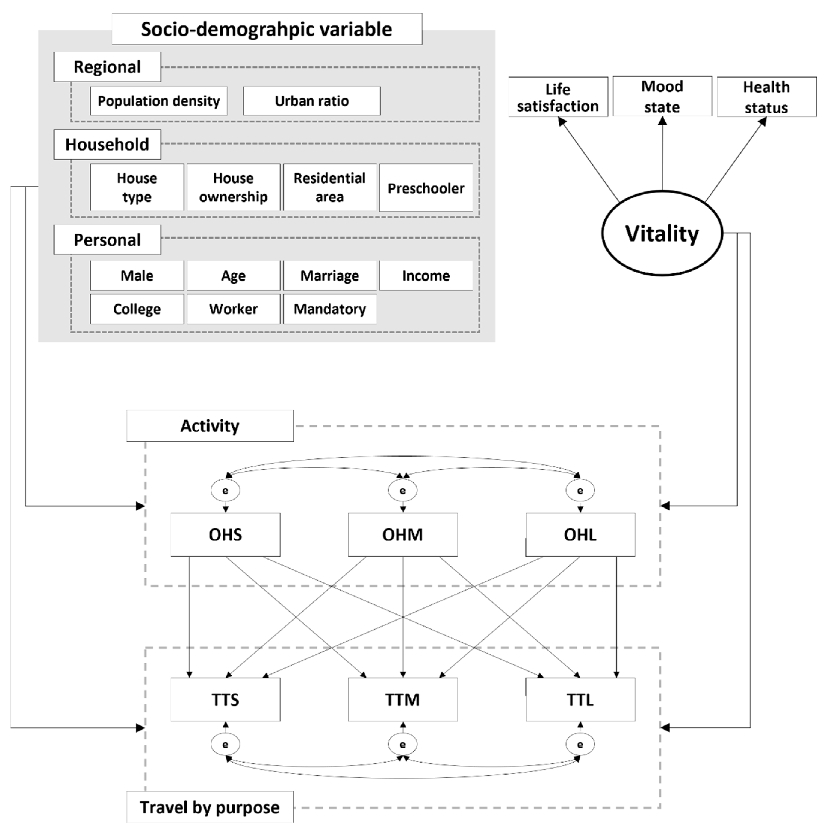
4.2. Model Structure

Six hypotheses were established for the construction of the structural model. Each hypothesis is formed based on the result obtained from prior studies and the research question raised in this study. The followings were our research hypotheses:

Hypothesis 1.

The error terms of the activity timeare correlated [19,20,21,22].

Hypothesis 2.

There is a correlation between the error terms of travel time by purpose [19,20,21,24].

Hypothesis 3.

The purpose of travel has a positive effect on the travel time [19,20,21,23,25].

Hypothesis 4.

All activities affect travel time [19,20,21,25].

Hypothesis 5.

The socio-demographic variables affect both activity and travel times [19,20,21,22,23,24,25,26].

Hypothesis 6.

Personal status affects both activity and travel times [27,29].

Based on these, a path model was developed, as illustrated in Figure 1. As shown in Table 2, the patterns of activity during weekdays and weekends are considerably different. We confirm that weekday data and weekend data were separately analyzed, but the structure of those models was similar. In the weekday model, 31,177 cases were used, while only 20,817 cases were used in the weekend model.

5. Result and Discussion

The study used the software Stata 16.0 to estimate SEM. We specifically chose the maximum likelihood estimation method that makes estimated results easier to interpret [19,39,40]. The results of the SEM are presented in

Table 3. Estimation result of the Structural Equation Model (Weekday).

Structural Model
Variables				OHS	OHM	OHL			TTS	TTM	TTL
Regional variables	Population density			−0.001 **	−7.87 × 10−5	0.001 **			0.001 **	−0.002 **	0.001 **
	Urbanization ratio			−1.82 × 10−5	1.44 × 10−4 **	−2.17 × 10−4 **			1.73 × 10−4 **	6.65 × 10−5	−1.68 × 10−4 **
Household variables	House type	House a		0.010 **	−0.004	0.002			−0.031 **	0.004	0.021 **
		Apartment a		−0.009 **	0.009 **	0.005			−0.015 **	−0.002	0.033 **
	House ownership	Own a		0.004	−0.015 **	0.019 **			−0.005	−0.013 **	0.020 **
		Monthly pay a		0.006 **	0.008 **	−0.013 **			0.007 *	0.005	−0.007
	Residential area			−1.09 × 10−4 **	1.70 × 10−5	3.75 × 10−5			−1.99 × 10−4 **	−1.07 × 10−4 **	3.15 × 10−4 **
	Preschooler a			−0.005 **	0.006 **	−0.037 **			−0.007 **	0.026 **	−0.043 **
Personal variables	Male a			0.004 **	−0.051 **	0.066 **			0.014 **	−0.027 **	0.006 *
	Age			−3.84 × 10−4 **	1.87 × 10−4 **	0.001 **			0.003 **	1.11 × 10−4	−0.004 **
	Marriage a			0.013 **	0.034 **	−0.058 **			0.025 **	0.050 **	−0.058 **
	College a			−0.008 **	0.006 **	−0.014 **			0.051 **	0.016 **	−0.065 **
	Worker a			0.034 **	0.018 **	−0.076 **			0.321 **	−0.011 **	−0.302 **
	Mandatory a			0.510 **	−0.134 **	−0.209 **			0.055 **	0.092 **	−0.265 **
	Income			0.010 **	0.003 **	−0.009 **			0.015 **	0.006 **	−0.007 **
Personal status	Vitality			−0.031 **	−0.011 **	0.064 **			−0.034 **	0.004	0.079 **
Activity time	OHS			-	-	-			0.764 **	−0.371 **	−0.140 **
	OHM			-	-	-			−0.082 **	0.768 **	−0.155 **
	OHL			-	-	-			−0.083 **	−0.319 **	0.625 **
Constant				0.037 **	0.266 **	0.373 **			−0.151 **	0.366 **	0.423 **
Measurement Model
Variables				Life satisfaction		Mood state				Health status
Vitality				1 (Constrained)		1.305 **				1.222 **
Constant				3.254 **		3.423 **				3.340 **
Covariance
TTS ↔ TTM: −0.016 **			TTS ↔ TTL: −0.021 **					TTM ↔ TTL: −0.019 **
OHS ↔ OHM: −0.005 **			OHS ↔ OHL: −0.009 **					OHM ↔ OHL: −0.015 **
Goodness-of-Fit
${\chi }^2$: 4701.823			RMSEA: 0.049				CFI: 0.977			TLI: 0.931

Note: ** = p-value ≤ 0.05, * = p-value ≤ 0.10; ^a It denotes that the variable is a dummy variable.

and

Table 4. Estimation result of the Structural Equation Model (Weekend).

Structural Model
Variables			OHS	OHM	OHL	TTS	TTM		TTL
Regional variables	Population density		−0.001 **	−0.001	0.002 **	3.65 × 10−4	−0.001		−0.001 *
	Urbanization ratio		−2.65 × 10−5	1.97 × 10−4 **	−2.75 × 10−4 **	8.69 × 10−5 **	1.25 × 10−4 *		−2.58 × 10−5
Household variables	House type	House a	0.015 **	−0.012 **	0.008	−0.022 **	0.014**		0.011
		Apartment a	−0.007 **	0.015 **	0.009	−4.24 × 10−4	0.012 *		0.018 **
	House ownership	Own a	0.009 **	−0.014 **	0.010 *	−0.007 **	−0.005		0.002
		Monthly pay a	0.005	0.008	−0.006	−0.002	−0.003		−0.009
	Residential area		−6.75 × 10−5 **	4.23 × 10−5	4.57 × 10−5	2.89 × 10−5	−4.33 × 10−6		7.51 × 10−5
	Preschooler a		−0.012 **	0.026 **	−0.038 **	0.001	0.020 **		−0.021 **
Personal variables	Male a		0.001	−0.062 **	0.089 **	0.012 **	−0.011 **		0.011 **
	Age		−4.83 × 10−5	−0.001 **	0.002 **	1.52 × 10−4 **	1.05 × 10−4		−0.001 **
	Marriage a		0.005 **	0.056 **	−0.076 **	−3.60 × 10−4	0.037 **		−0.020 **
	College a		−0.012 **	0.013 **	−0.003	−0.004	0.016 **		−0.004
	Worker a		0.003	0.045 **	−0.040 **	0.004	0.026 **		0.012 **
	Mandatory a		0.535 **	−0.135 **	−0.226 **	0.211 **	0.091 **		−0.001
	Income		0.002 **	0.006 **	−0.010 **	0.004 **	0.001		3.67 × 10−4
Personal status	Vitality		−0.021 **	0.021 **	0.066 **	−0.013 **	0.027 **		0.090 **
Activity time	OHS		-	-	-	0.846 **	−0.217 **		−0.158 **
	OHM		-	-	-	−0.013 **	0.922 **		−0.106 **
	OHL		-	-	-	−0.021 **	−0.176 **		0.709 **
Constant			0.020 **	0.250 **	0.313 **	0.001	0.172 **		0.223 **
Measurement Model
Variables			Life satisfaction		Mood state		Health status
Vitality			1 (Constrained)		1.510 **		1.294 **
Constant			3.251 **		3.556 **		3.394 **
Covariance
TTS ↔ TTM: −0.008 **			TTS ↔ TTL: −0.006 **			TTM ↔ TTL: −0.031 **
OHS ↔ OHM: −0.004 **			OHS ↔ OHL: −0.007 **			OHM ↔ OHL: −0.024 **
Goodness-of-Fit
${\chi }^2$: 3232.256			RMSEA: 0.049		CFI: 0.973			TLI: 0.919

Note: ** = p-value ≤ 0.05, * = p-value ≤ 0.10. ^a It denotes that the variable is a dummy variable.

. We first explored the goodness-of-fit. There are various goodness-of-fit measures in evaluating SEMs, including the absolute fit, incremental fit, and parsimonious fit measure. The absolute fit measure, which is based on the theory of covariance matrixes, is an index that shows how much the model predicts the sample covariance matrix. Typical indicators are the Chi-square (${\chi }^2$), Root Mean Square Residual (RMR), Goodness-of-Fit Index (GFI), and Root Mean Square Error of Approximation (RMSEA). The incremental fit measure is an index indicating how well the study model was measured compared to the null model. The index consists of the Normal Fit Index (NFI), Relative Fit Index (RFI), Incremental Fit Index (IFI), Turker–Lexis Index (TLI), and Comparative Fit Index (CFI). The parsimonious fit measures contain the complexity of the model and is used in a comparison between models. In general, there are the Parsimony RATIO (PRATIO), Parsimonious GFI (PGFI), Parsimonious NFI (PNFI), and Parsimonious CFI (PCFI). In this study, the model fit measurement was verified with absolute and incremental fit measures given that comparisons between models were not performed [33,34,35,38].

In the absolute fit measure, we used RMSEA. For Chi-square, it is susceptible to sample size, and it is easy to reject the null hypothesis that “the model is appropriate” when the sample size is larger than 200 [33,38]. Since more than 200 cases were utilized in this study, RMSEA was adopted to complement the problem with the Chi-square statistics. RMSEA has the advantage of being less affected by sample size. It is generally considered a good model when RMSEA is under 0.05 [34,35]. The most basic index in the incremental fit measure is NFI. This index indicates how much improvement the proposed model has made over the null model. It ranges between 0 and 1, and the closer it is to 1, the better it is. Recently, CFI and TLI have been mainly recommended rather than NFI; thus, these two indices were used in this study. CFI and TLI, like NFI, have a range from 0 to 1, and models can be considered acceptable when the value is over 0.9 [34,35]. As a result of the model fit analysis, we confirmed that both weekday and weekend models satisfied RMSEA < 0.05, CFL > 0.9, and TLI > 0.9. All models were statistically significant and represented approximations close to the population.

Table 3 and Table 4 show the result of the final SEM. First of all, there were more significant variables in the weekday model compared to the weekend one. This was probably because people’s lifestyles are more similar during the weekday than those during the weekend [1]. For example, most people are likely to work or study during weekdays while enjoying a variety of leisure activities on weekends. Not surprisingly, most of the variables showed the same relationship with expected signs during the weekdays and weekends, but the magnitudes of coefficients were fairly different (refer to our interpretation and justification in Section 5.2). With respect to the regional variables, it was found that the population density and urbanization ratio had opposite effects. We contemplated that this was because popularized areas are mostly placed in urban areas; accordingly, the lower the urbanization ratio is, the higher the population density is. In case of the personal variables, more variables other than household variables were found to be significant. Since the Time Use Survey investigated individual behavioral characteristics, we can safely assume that it was more influenced by personal traits rather than household ones. We demonstrated that personal status affected both activity travel times and vice versa. The latent variable, vitality, that reflects personal status influenced both activity and travel times as well. Each activity time also affected the travel time across purposes.

5.1. Hypothesis Test

As described in Section 4.2, six hypotheses were established for the SEM analysis and successfully verified. The following paragraphs provide detailed descriptions and corresponding estimation results of each hypothesis.

Hypothesis 1.

The error terms of the activity time have a correlation [19,20,21,22].

Correlation analysis between activity times showed that the error terms between all activities were negatively correlated. This aligns with Chung and Ahn’s findings that the activity times of other activities negatively affect each other [19]. From a conventional perspective, this finding can be accepted, since the total amount of one day time is fixed at 24 h.

Hypothesis 2.

There is a correlation between the error terms of travel time by purpose [19,20,21,24].

The correlation analysis between the ratio of travel time by purpose showed that there was a correlation between the error terms of the travel time ratio for all purposes. All coefficients had a negative effect. This is consistent with the theory of the travel time budget [41], in which the total travel time is set relatively constant and the designated travel times are divided by purpose.

Hypothesis 3.

The purpose of travel has a positive effect on the travel time [19,20,21,23,25].

In the travel time model, all the purpose-specific activity times had a positive effect, which parallels Sharmeen et al. [20]. Given that travel is a derived demand, it is believed that the travel time for each purpose increases depending on the activities relevant to the purpose [8,9].

Hypothesis 4.

All activities affect travel time [19,20,21,25].

Neither the activity time for the purpose nor the time of activity affected the travel time. Activity times disassociated with travel were found to have a negative effect on travel time, which is straightforward, because both activities and travel occur during the day.

Hypothesis 5.

The socio-demographic variables affect both the activity and the travel times [19,20,21,22,23,24,25,26].

There were 13 socio-demographic variables incorporated into the model. Unfortunately, not all variables were significant in all models, but most turned out to be significant variables.

Hypothesis 6.

Personal status affects both the activity and the travel times [27,29].

Personal status affected both the activity and travel times. Especially, personal status had a significant impact on the activity and travel times with the same direction for the activity purpose. We could find similar cases. Several previous studies defining individual characteristics as latent variables showed that individual moods and conditions have an influence on activities [27,29].

5.2. Total, Direct, and Indirect Effect Analysis

To analyze the influence of each variable on travel time by purpose, direct, indirect, and total effects were identified, as shown in

Table 5. Total, Direct, and Indirect Effects by type of week.

Variable		Weekday			Weekend
		Total Effect	Direct Effect	Indirect Effect	Total Effect	Direct Effect	Indirect Effect
TTS ←	Population Density	−3.64 × 10−5	0.001 **	−0.001 **	−3.31 × 10−4	3.65 × 10−4	−0.001 **
	Urbanization Ratio	1.65 × 10−4 **	1.73 × 10−4 **	−7.61 × 10−6	6.78 × 10−5	8.69 × 10−5 **	−1.91 × 10−5
	House a	−0.023 **	−0.031 **	0.008 **	−0.010 **	−0.022 **	0.013 **
	Apartment a	−0.023 **	−0.015 **	−0.008 **	−0.007	−4.24 × 10−4	−0.006 **
	Own a	−0.002	−0.005	0.002	4.69 × 10−4	−0.007 **	0.007 **
	Monthly Pay a	0.013 **	0.007 *	0.005 **	0.002	−0.002	0.004
	Residential Area	−2.87 × 10−4 **	−1.99 × 10−4 **	−8.81 × 10−5 **	−2.97 × 10−5	2.89 × 10−5	−5.87 × 10−5 **
	Preschooler a	−0.008 **	−0.007 **	−0.001	−0.008 **	0.001	−0.009 **
	Male a	0.016 **	0.014 **	0.002	0.012 **	0.012 **	−7.12 × 10−5
	Age	0.002 **	0.003 **	−3.47 × 10−4 **	8.19 × 10−5	1.52 × 10−4 **	−7.05 × 10−5
	Marriage a	0.037 **	0.025 **	0.012 **	0.005	−3.60 × 10−4	0.005 **
	College a	0.045 **	0.051 **	−0.006 **	−0.014 **	−0.004	−0.010 **
	Worker a	0.352 **	0.321 **	0.031 **	0.006 *	0.004	0.002
	Mandatory a	0.473 **	0.055 **	0.418 **	0.671 **	0.211 **	0.459 **
	Income	0.024 **	0.015 **	0.008 **	0.006 **	0.004 **	0.002 **
	Vitality	−0.062 **	−0.034 **	−0.028 **	−0.033 **	−0.013 **	−0.020 **
	OHS	0.764 **	0.764 **	(No Path)	0.846 **	0.846 **	(No Path)
	OHM	−0.082 **	−0.082 **	(No Path)	−0.013 **	−0.013 **	(No Path)
	OHL	−0.083 **	−0.083 **	(No Path)	−0.021 **	−0.021 **	(No Path)
TTM ←	Population Density	−0.002 **	−0.002 **	−1.84 × 10−6	−0.002 **	−0.001	−0.001
	Urbanization Ratio	2.53 × 10−4 **	6.65 × 10−5	1.86 × 10−4 **	3.61 × 10−4 **	1.25 × 10−4 *	2.36 × 10−4 **
	House a	−0.004	0.004	−0.007 **	−0.002	0.014 **	−0.016 **
	Apartment a	0.007	−0.002	0.008 **	0.026 **	0.012 *	0.014 **
	Own a	−0.032 **	−0.013 **	−0.019 **	−0.022 **	−0.005	−0.017 **
	Monthly Pay a	0.013 **	0.005	0.008 **	0.004	−0.003	0.007
	Residential Area	−6.52 × 10−5	−1.07 × 10−4 **	4.17 × 10−5	4.13 × 10−5	−4.33 × 10−6	4.56 × 10−5
	Preschooler a	0.044 **	0.026 **	0.019 **	0.053 **	0.020 **	0.033 **
	Male a	−0.089 **	−0.027 **	−0.062 **	−0.085 **	−0.011 **	−0.073 **
	Age	−1.54 × 10−4	1.11 × 10−4	−2.65 × 10−4 **	−0.001 **	1.05 × 10−4	−0.001 **
	Marriage a	0.090 **	0.050 **	0.040 **	0.101 **	0.037 **	0.064 **
	College a	0.028 **	0.016 **	0.012 **	0.031 **	0.016 **	0.015 **
	Worker a	0.015 **	−0.011 **	0.026 **	0.074 **	0.026 **	0.048 **
	Mandatory a	0.318 **	0.092 **	0.226 **	0.292 **	0.091 **	0.201 **
	Income	0.007 **	0.006 **	0.001	0.008 **	0.001	0.007 **
	Vitality	−0.013 **	0.004	−0.018 **	0.039 **	0.027 **	0.012 **
	OHS	−0.371 **	−0.371 **	(No Path)	−0.217 **	−0.217 **	(No Path)
	OHM	0.768 **	0.768 **	(No Path)	0.922 **	0.922 **	(No Path)
	OHL	−0.319 **	−0.319 **	(No Path)	−0.176 **	−0.176 **	(No Path)
TTL ←	Population Density	0.002 **	0.001 **	0.001 **	0.001	−0.001 *	0.002 **
	Urbanization Ratio	−3.24 × 10−4 **	−1.68 × 10−4 **	−1.55 × 10−4 **	−2.38 × 10−4 **	−2.58 × 10−5	−2.12 × 10−4 **
	House a	0.021 **	0.021 **	3.79 × 10−4	0.015 *	0.011	0.004
	Apartment a	0.036 **	0.033 **	0.003	0.023 **	0.018 **	0.006
	Own a	0.033 **	0.020 **	0.014 **	0.009	0.002	0.007 *
	Monthly Pay a	−0.017 **	−0.007	−0.011 **	−0.015 *	−0.009	−0.006
	Residential Area	3.51 × 10−4 **	3.15 × 10−4 **	3.61 × 10−5 *	1.14 × 10−4 *	7.51 × 10−5	3.86 × 10−5
	Preschooler a	−0.066 **	−0.043 **	−0.023 **	−0.049 **	−0.021 **	−0.028 **
	Male a	0.055 **	0.006 *	0.049 **	0.081 **	0.011 **	0.070 **
	Age	−0.003 **	−0.004 **	0.001 **	−1.32 × 10−4	−0.001 **	0.001 **
	Marriage a	−0.102 **	−0.058 **	−0.043 **	−0.081 **	−0.020 **	−0.060 **
	College a	−0.073 **	−0.065 **	−0.008 **	−0.005	−0.004	−0.002
	Worker a	−0.357 **	−0.302 **	−0.055 **	−0.022 **	0.012 **	−0.034 **
	Mandatory a	−0.446 **	−0.265 **	−0.181 **	−0.231 **	−0.001	−0.230 **
	Income	−0.015 **	−0.007 **	−0.008 **	−0.008 **	3.67 × 10−4	−0.008 **
	Vitality	0.125 **	0.079 **	0.046 **	0.138 **	0.090 **	0.048 **
	OHS	−0.140 **	−0.140 **	(No Path)	−0.158 **	−0.158 **	(No Path)
	OHM	−0.155 **	−0.155 **	(No Path)	−0.106 **	−0.106 **	(No Path)
	OHL	0.625 **	0.625 **	(No Path)	0.709 **	0.709 **	(No Path)

Note: ** = p-value ≤ 0.05, * = p-value ≤ 0.10. ^a It denotes that the variable is a dummy variable.

. In most variables, the direction of the coefficients of total and direct effects was identical. In the weekend model, there were more cases where the direction of the coefficient of the total effect and the direct effect were different. One possible explanation is that activity patterns are more diverse on weekends than weekdays, hinting that there are more unobserved factors which were not included in the present model [1]. In the weekday model, workers showed a positive effect on the total effect and a negative effect on the direct effect on the TTM. Workers usually perform work activities and generate relevant commuting trips as well during the weekday. An increase in travel time for work decreases travel time for maintenance. This makes the worker have a negative direct effect on the TTM. Maintenance activity (OHM) includes activities such as getting ready to go out and having lunch. As workers commute to work, they perform maintenance activities that increase OHM. An increase in OHM also increases TTL; thus, workers indirectly increase TTL. In the weekend model, workers had a positive effect on the total effect and a negative effect on the direct effect on TTL. Having an income allows workers to have more opportunities to move, which leads to a positive direct effect on TTL [23]. Since workers mostly have relatively less time for leisure activities [20], however, the total effect turned out to be negative.

In the total effect analysis, most variables showed the same direction in the weekday and weekend models, except for some variables. College, indicating whether a student has graduated from college, had a positive effect on TTS in the weekday model and a negative effect in the weekend model. In general, it is assumed that commuting to work is longer than commuting to school, because schools are usually located closer to residential areas, especially in South Korea. This is why college had a positive effect on TTS in the weekday model while the coefficient of college was negative in the weekend model. On weekends, the decrease in working time is greater than the decrease in time spent on study, which resulted in the negative coefficient of college. In the weekday model, the indirect effect was negative because college has a negative impact on OHS. According to the Korean Labor Law [41], working times are limited to 52 h per week, whereas there is no restriction on study time (note that K-12 students spend over 50 h, on average, per week on study [42]). In other words, the subsistence activity time of students is longer than that of the worker, leading to the negative indirect effect of college. Vitality showed a negative effect on TTM in the weekday model and a positive effect in the weekend model, which was the same as the effect on OHM. Maintenance activities include getting ready to go out and cleaning the house. During the week, these activities have similar characteristics to subsistence activities, such as preparing for work and cleaning up the house after working when there is insufficient time. When OHM is performed on the weekend, it has similar characteristics to leisure activities, such as preparing for leisure activities and cleaning the house when there is time to spare. Accordingly, it had a negative effect on weekdays like OHS and a positive effect on weekends like OHL.

Regional variables (i.e., population density and urbanization ratio) showed opposite effects. Since an increase in the urbanization ratio decreases the population density, it can be interpreted that the influence of the urbanization ratio and the population density were reversed. The high urbanization ratio means that the city area is relatively large (and of course, most people live in urban areas). Assuming the same population, if the urban area is large, the population density can decrease. Population density had a negative effect on both TTS and TTM and a positive effect on TTL. This means that most of the urban areas have facilities supporting subsistence and maintenance activities, and it can be interpreted that leisure facilities are located relatively outside of the city center.

Regarding the household variables, there was a discrepancy in the coefficients by house type, but the direction of the influence was the same. House ownership (Own) and residential area had a negative effect on TTS and a positive effect on TTL, whereas house ownership (Monthly pay) showed an opposite effect. A person who owns a house and lives in a large residential area can be viewed as a member of a high-income household. Higher household income could lead to increasing leisure activity times by providing opportunities for various activities. It increases the ratio of travel time for leisure and thus reduces the ratio of travel time for subsistence. As expected, people with preschoolers need extra time to take care of their children, which has a positive effect on TTM and a negative effect on both TTS and TTL. Among personal variables, being male showed a positive effect on TTS, which was expected given that there are more male workers than female workers. TTL also showed that being male had a positive effect, which was presumably because female’s leisure activities are mainly done at home [32]. As people get older, people tend to retire and enjoy leisure. This tendency could make age have a negative effect on OHS and a positive effect on OHL. Likewise, age would be expected to have a negative effect on TTS and a positive effect on TTL, but the result was opposite from our expectation. According to a decrease of OHS and increase of OHL, the indirect effect appeared to be the same as expected, but the result was different due to the direct effect. As we age, travel becomes more inconvenient, leading to a shortening travel distance [43]. In the case of travel for maintenance and leisure, the destination of the activity may be replaced by other places closer to origin. However, the destination of travel for subsistence is difficult to change. Therefore, as maintenance and leisure travel distances decrease, the subsistence travel ratio increases relatively. Marriage had a positive effect on TTS and TTM and a negative effect on TTL [20,25]. This was maybe because marriage increases responsibility and activities related to family obligation. As expected, college, worker, and mandatory had an influence in the same direction, which was the same result proposed by [19,20,24]. Subsistence activity increased according to the above three variables (college, worker, mandatory) and thus had a positive effect on TTS and TTM and a negative effect on TTL. Unlike household income indicators such as house ownership and residential area, personal income (variable Income) had a positive effect on TTS and TTM and a negative effect on TTL. An increase in income has two effects. One is an increase in opportunities for various leisure activities and an increase leisure time [19] and the other is an increase in working time [25]. Income growth is more affected by increased working times. However, household income may increase as the personal income of other household members increase, and in this case, an increase in working time does not increase income. This is why house ownership and residential area showed different directions to income.

The variable vitality, indicating personal status, had a negative effect on TTS and a positive effect on TTL. Vitality is a latent variable that measures an individual’s state, such as health and mood. Therefore, a high vitality means a person who is energetic and healthy. It is generally known that people perform more leisure activities when the vitality is high, which may lead to fewer subsistence activities [27,29].

Since there is no indirect effect on activity times, the total effect and the direct effect are the same. In all ratios of travel time across purpose, activities belonging to the specific purpose of travel showed a positive effect. This means that travel has the nature of derived demand [8,9]. In the case of activities not belonging to travel, negative effects were observed, and all of them were significant. This implies that (1) travel time is also affected by the time constraint (24 h per day) and that (2) non-travel related activities also affect travel. Except for the activity time spent on the corresponding travel purpose, all activity time (including the travel time for other purposes) have a negative effect on the travel time, concluding that travel time is viewed as a disutility in most cases [3,6,7].

6. Conclusions

In this study, the causal relationship between activity and travel times was analyzed using 2019 Time Use Survey data in Korea. Six hypotheses were established to develop the structural equation model (SEM). The key findings and relevant implications of this research can be summarized as follows.

First, the effects on travel time were analyzed by diving them into direct and indirect effects. The direct and indirect effects of most variables provided the same direction of coefficients, but some variables (e.g., age, college, and worker) showed a discrepancy in the directions of effects. This means that factors affecting travel have not only a direct effect, but also an indirect effect for various reasons. In addition, there were cases where the indirect effect was greater than the direct effect. In this regard, we can infer that those variables have indirect effects as well as direct effects; in particular, indirect effects are important as much as direct effects.

Second, all activities could affect travel time. Given that travel is a derived demand, we used an activity-based travel model and took only the travel purpose into account as an influential factor affecting travel time. Previous studies and empirical attempts have tended to consider only activities for travel purposes when drawing a transportation policy. However, this study found that all types of activities affect travel time, proposing that future transportation policies need to be established after the consideration of various activities.

Third, travel has both utility and disutility at the same time. In early travel-related studies, travel was considered a disutility, and a vast majority of those studies focused on minimizing travel time. However, travel has recently been considered as a utility that provides opportunities for various activities, depending on the context of location, purpose, and personality. Previous studies were likely to choose a single perspective between utility and disutility. However, our results demonstrated that travel has both utility and disutility at the same time, suggesting a new point of view. For example, the parking fee increase policy should be carried out with an increase in public transportation services. The increase in parking fees reduces passenger car traffic and shortens the travel time according to the decrease in road traffic. However, as passenger car traffic decreases, it becomes inconvenient to move to other places. Therefore, it is necessary to improve public transportation services in order to increase the convenience of movement.

Fourth, personal status affects the travel time ratio. In most prior studies, only socio-economic indicators such as gender, age, and income were used when performing travel time-related studies. On the contrary, this study incorporated a latent variable, vitality, and it was found to affect the travel time ratio. This means that individual tendencies are reflected (partly at least) in people’s travel patterns. Therefore, individual tendencies should be considered in future travel-related research and policy establishment. When planning a city, a specific strategy can be established after consideration of the difference in the activity-specific vitality. Given that work activities mostly lower vitality and leisure activities increase vitality, residential and business areas can be located closely. Likewise, residential and leisure areas can be placed farther than the aforementioned geographic location.

Fifth, activity and travel times show a complex causal relationship. Since various activities and relevant travel can contribute to live, active cities, it is imperative to examine the casual relationship between activity and travel when planning urban and transportation infrastructure. Within the frame of this, we hope that this study can help to decide on the location of electric charging stations. Specifically, a substantial number of studies have been conducted focusing on the location choice of electric charging stations and electric batteries [44,45,46,47]. Electric vehicle battery charging can be viewed as a specific maintenance activity; an increase in maintenance activity time could reduce leisure travel time more than subsistence travel time. This can be treated as reducing leisure travel time to charge electric vehicle batteries. The decrease in leisure travel time means that movement for leisure activities is reduced, which reduces the opportunity for leisure activities to occur. Therefore, as a way to prevent this, it is possible to establish a plan to locate an electric charging station near leisure areas.

We used Time Use Survey data, which only investigated respondents’ residences at the city level, but we did not collect information about origin and destination. In the future, a sophisticated survey design at a deeper level is called for for investigating detailed information. For example, if it is possible to subdivide aggregated traffic zones into small pieces, indicators such as the number of workers, spatial abundance, Infrastructure status, and public transportation facilities can be identified [30,31]. We also expect that an origin and destination survey will allow us to further specify regional characteristics of the origin and destination. Lastly, we did not focus on travel mode, although travel time is commonly associated with travel mode. Thus, considering travel mode in analyzing the differences in travel mode according to activities for travel purposes and the characteristics of travel time by travel mode will be useful to improve models.

References

1. McBridem, E.C.; Davis, A.W.; Goulias, K.G. Exploration of Statewide Fragmentation of Activity and Travel and a Taxonomy of Daily Time Use Patterns using Sequence Analysis in California. Transp. Res. Rec. 2020, 2674, 38–51. [Google Scholar] [CrossRef]
2. Kitamura, R. An Evaluation of Activity-Based Travel Analysis. Transportation 1988, 15, 9–34. [Google Scholar] [CrossRef]
3. Axhausen, K.W.; Garling, T. Activity-Based Approaches to Travel Analysis: Conceptural Frameworks, Models and Research Problems. Transp. Rev. 1992, 12, 323–341. [Google Scholar] [CrossRef] [Green Version]
4. Golob, T.F. A Simultaneous Model of Household Activity Participation and Trip Chain Generation. Transp. Res. Part B Methodol. 2000, 34, 355–376. [Google Scholar] [CrossRef] [Green Version]
5. Rasouli, S.; Timmermans, H. Activity-Based Models of Travel Demand: Promises, Progress and Prospects. Int. J. Urban Sci. 2014, 18, 31–60. [Google Scholar] [CrossRef]
6. Stephan, G.E.; Tedrow, L.M. A Theory of Time-Minimization: The Relationship between Urban Area and Population. Pac. Sociol. Rev. 1977, 20, 105–112. [Google Scholar] [CrossRef]
7. Recker, W.W.; McNally, M.G.; Root, G.S. A Model of Complex Travel Behavior: Part Ⅰ-Theroetical Development. Transp. Res. Part A Gen. 1986, 20, 307–318. [Google Scholar] [CrossRef]
8. Dijst, M.; Vidakovic, V. Travel Time Ratio: The Key Factor of Spatial Reach. Transportation 2000, 27, 179–199. [Google Scholar] [CrossRef]
9. Morris, J.M.; Dumble, P.L.; Wigan, M.R. Accessibility Indicators for Transport Planning. Transp. Res. Part A Gen. 1979, 13, 91–109. [Google Scholar] [CrossRef]
10. Hamed, M.M.; Mannering, F.L. Modeling Travelers’ Postwork Activity Involvement: Toward a New Methodology. Transp. Sci. 1993, 27, 381–394. [Google Scholar] [CrossRef]
11. Schwanen, T.; Dijst, M. Travel-time Ratios for Visits to the Workplace: The Relationship between Commuting Time and Work Duration. Transp. Res. Part A Policy Pract. 2002, 36, 573–592. [Google Scholar] [CrossRef]
12. Susilo, Y.; Dijst, M. How Far is Too Far? Travel time ratios for activity participation in the Netherlands. Transp. Res. Rec. J. Transp. Res. Board 2009, 2134, 89–98. [Google Scholar] [CrossRef]
13. Tanner, J.C. Factors Affecting the Amount of Travel; HM Stationery Office: London, UK, 1961.
14. Szalai, A. The Use of Time: Daily Activities of Urban and Suburban Populations in Twelve Countries. J. Leis. Res. 1972, 6, 84–86. [Google Scholar]
15. Zahavi, Y. The TT-relationship: A Unified Approach to Transportation Planning. Traffic Eng. Control. 1973, 15, 205–212. [Google Scholar]
16. Zahavi, Y. Traveltime Budgets and Mobility in Urban Areas; U.S. Department of Transportation: Washington, DC, USA, 1974.
17. Schafer, A.; Victor, D.G. The Future Mobility of the World Population. Transp. Res. Part A 2000, 34, 171–205. [Google Scholar] [CrossRef]
18. Kitamura, R.; Fujii, S. Time-use Data, Analysis and Modeling: Toward the Nest Generation of Transportation Planning Methodologies. Transp. Policy 1997, 4, 225–235. [Google Scholar] [CrossRef]
19. Chung, J.H.; Ahn, Y. Structural Equation Models of Day-to-Day Activity Participation and Travel Behavior in a Developing Country. Transp. Res. Rec. 2002, 1807, 109–118. [Google Scholar] [CrossRef]
20. Sharmeen, F.; Arentze, T.; Timmermans, H. Incorporating Time Dynamics in Activity Travel Behavior Model: A Path analysis of Change in Activity and Travel Time Allocation in Response to Life-Cycle Events. Transp. Res. Rec. 2013, 2382, 54–62. [Google Scholar] [CrossRef]
21. Manoj, M.; Verma, A. A Structural Equation Model Based Analysis of Non-Workers’ Activity-Travel Behaviour from a City of a Developing Country. Transportation 2017, 44, 241–269. [Google Scholar] [CrossRef]
22. Ziems, S.E.; Konduri, K.C.; Sana, B.; Pendyala, R.M. Exploration of Time Use Utility Derived by Older Individuals from Daily Activity-Travel Patterns. Transp. Res. Rec. 2010, 2156, 111–119. [Google Scholar] [CrossRef]
23. Lizana, M.; Carrasco, J.A.; Victoriano, R. Daily Activity-Travel and Fragmention patterns in the Weekly Cycle: Evidence of the Role of ICT, Time Use, and Personal Networks. Transp. Lett. 2021, 1–11. [Google Scholar] [CrossRef]
24. Simma, A.; Axhausen, K.W. Within-Household Allocation of Travel: Case of Upper Austria. Transp. Res. Rec. 2001, 1752, 69–75. [Google Scholar] [CrossRef]
25. Soo, J.; Ettema, D.; Ottens, H.F.L. Analysis of Travel Time in Multiple-Purpose Trips. Transp. Res. Rec. 2008, 2082, 56–62. [Google Scholar] [CrossRef]
26. Raux, C.; Ma, T.Y.; Joly, I.; Kaufmann, V.; Cornelis, E.; Ovtracht, N. Travel and Activity Time Allocation: An Empirical Comparison between Eight Cities in Europe. Transp. Policy 2011, 18, 401–412. [Google Scholar] [CrossRef] [Green Version]
27. Huang, S.; Hsu, C.H. Effects of Travel Motivation, Past Experience, Perceived Constraint, and Attitude on Revisit Intention. J. Travel Res. 2009, 48, 29–44. [Google Scholar] [CrossRef]
28. Lin, T.; Wang, D.; Guan, X. The Built Environment, Travel Attitude, and Travel Behavior: Residential Self-selection or Residential Determination? J. Transp. Geogr. 2017, 65, 111–122. [Google Scholar] [CrossRef]
29. De Vos, J.; Singleton, P.A.; Garling, T. From Attitude to Satisfaction: Introducing the Travel Mode Choice Cycle. Transp. Rev. 2022, 42, 204–221. [Google Scholar] [CrossRef]
30. Najaf, P.; Thill, J.C.; Zhang, W.; Fields, M.G. City-level Urban Form and Traffic Safety: A Structural Equation Modeling Analysis of Direct and Indirect Effects. J. Transp. Geogr. 2018, 69, 257–270. [Google Scholar] [CrossRef]
31. Zhang, W.; Lu, D.; Zhao, Y.; Luo, X.; Yin, J. Incorporating Polycentric Development and Neighborhood Life-circle Planning for Reducing Driving in Beijing: Nonlinear and Threshold Analysis. Cities 2022, 121, 103488. [Google Scholar] [CrossRef]
32. Ministry of Culture, Sport and Tourism. National Leisure Activity Survey; Ministry of Culture, Sport and Tourism: Sejong Special Self-Governing City, Korea, 2019.
33. Schumacker, R.E.; Lomax, R.G. A Beginner’s Guide to Structural Equation Modeling, 4th ed.; Routledge: London, UK, 2016. [Google Scholar]
34. Briwbe, M.W.; Cudeck, R. Alternative Ways of Assessing Model Fit. Sociol. Methods Res. 1992, 21, 230–258. [Google Scholar]
35. Hu, L.T.; Bentler, P.M. Couoff Criteria for Fit Indexes in Covariance Structure Analysis: Conventional Criteria Versus New Alternatives. Struct. Equ. Modeling A Multidiscip. J. 1999, 6, 1–55. [Google Scholar] [CrossRef]
36. Bollen, K.; Pearl, J. Eight Myths about Causality and Structural Equation Models. In Handbook of Casual Analysis for Social Research; Springer: Dordrecht, The Netherlands, 2013; pp. 301–328. [Google Scholar]
37. Mueller, R. Basic Principles of Structural Equation Modeling: An Introduction to LISREL and EQS; Springer: New York, NY, USA, 1996. [Google Scholar]
38. Byrne, B.M. Structural Equation Modeling with Lisrel, Prelis, and Simplis. In Basic Concepts, Applications, and Programming; Lawrence Erlbaum Associates: Mahwah, NJ, USA, 1998. [Google Scholar]
39. Golob, T.F.; McNally, G. A Model of Activity Participation and Travel Interactions between Household Heads. Transp. Res. Part B Methodol. 1997, 31, 177–194. [Google Scholar] [CrossRef] [Green Version]
40. Lu, X.; Pas, E.I. Socio-Demographics, Activity Participation and Travel Behavior. Transp. Res. Part A Policy Pract. 1999, 33, 1–18. [Google Scholar] [CrossRef]
41. Korean Ministry of Government Legislation. Available online: www.law.go.kr (accessed on 3 March 2022).
42. OECD. PISA 2018: Insights and Interpretations; OECD: Paris, France, 2019. [Google Scholar]
43. Shao, F.; Sui, Y.; Sun, R. Spatio-temporal Travel Patterns of Elderly People—A Compartive Study Based on Buses Usage in Qingdao, China. J. Transp. Geogr. 2019, 76, 178–190. [Google Scholar] [CrossRef]
44. Ahmadian, A.; Sedghi, M.; Golkar, M.A. Stochastic Modeling of Plug-in Electric Vehicles Load Demand in Residential Grids Considering Nonlinear Battery Charge Characteristic. In Proceedings of the 20th Iranian Electrical Power Distribution Conference, Zahedan, Iran, 28–29 April 2015. [Google Scholar]
45. Ahmadian, A.; Ivatloo, B.M.; Elkamel, A. A Review on Plug-in Electric Vehicles: Introduction, Current Status, and Load Modeling Techniques. J. Mod. Power Syst. Clean Energy 2020, 8, 412–425. [Google Scholar] [CrossRef]
46. Jahngir, H.; Gougheri, S.S.; Vatandoust, B.; Golkar, M.A.; Ahmadian, A.; Hajizadeh, A. Plug-in Electric Vehicle Behavior Modeling in Energy Market: A Novel Deep Learning-Based Approach with Clustering Technique. IEEE Trans. Smart Grid 2020, 11, 4738–4748. [Google Scholar] [CrossRef]
47. Saatloo, A.M.; Moradzadeh, A.; Ivatloo, B.M.; Ahmadian, A.; Elkamel, A. Machine Learning Based PEVs Load Extraction and Analysis. Electronics 2020, 9, 1150. [Google Scholar] [CrossRef]
Figure 1. Structure of the final SEM.
Sustainability 14 04615 g001