Article

A Novel Approach to Generate Hourly Photovoltaic Power Scenarios

1
Department of Mathematics, Natural and Economic Sciences, Ulm University of Applied Sciences, 89075 Ulm, Germany
2
Center for Solar Energy and Hydrogen Research Baden-Württemberg, 89075 Ulm, Germany
3
Institute of Economic Sciences, 11000 Belgrade, Serbia
*
Author to whom correspondence should be addressed.
Sustainability 2022, 14(8), 4617; https://doi.org/10.3390/su14084617
Submission received: 14 March 2022 / Revised: 6 April 2022 / Accepted: 11 April 2022 / Published: 12 April 2022

Abstract

:
Photovoltaic power is playing an ever-increasing role in the energy mix of countries worldwide. It is a stochastic energy source, and simulation models are needed to establish reliable risk management. This paper presents a novel approach for simulating hourly solar irradiation and—as a consequence—photovoltaic power based on easily accessible data such as wind, temperature, and cloudiness. Solar simulations are generated via a multiplication factor that scales the maximum possible solar irradiation. Photovoltaic simulations are then derived using formulas that approximate the physical interdependencies. The resulting simulations are unbiased on an annual level and reasonably reflect historic irradiation movements. Interpreting our approach as a descriptive model, we find that error values vary over the year and with granularity. Errors are highest when considering hourly values in wintertime, especially in the morning or late afternoon.

1. Introduction

Climate change is a major concern for the international community, with global warming being among the most visible effects [1]. In recent years, governments have been increasing efforts to fight climate change and global warming, and hence environmental degradation—challenges that confront modern society and cause numerous problems [2,3]. Thereby, the focus primarily lies on significantly reducing greenhouse gas emissions. Transforming energy production towards an (almost) carbon-neutral future becomes essential in this context. However, challenges are ample. Financial costs are considerable, and it remains challenging to integrate renewable energy into the electricity grid on a large scale [4,5]. The primary reason is that weather is stochastic, and so is wind or photovoltaic energy. Power utilities have to provide backups to prevent blackouts; companies and more minor participants such as individual households have to calculate with uncertain profits when deciding about investments in renewable energies such as rooftop solar panels.
Regarding photovoltaic power, there are numerous commercial and non-commercial tools for calculating the financial value of a solar panel. To the authors’ best knowledge, these tools are exclusively based on historical weather observations and yield an average payoff for a panel. No risk analysis such as computing quantile values is possible for deciding about substantial financial investments with amortization periods of 10–20 years—an aspect that is becoming even more important in Germany as feed-in tariffs and, subsequently, profitability are decreasing.
The literature already offers some approaches to simulate photovoltaic power (see Section 2 and the discussion in Section 5.2), which is a challenging task. The output of a photovoltaic panel is influenced, among other things, by temperature, air pressure, aerosol optical density, precipitation, ozone concentration, and humidity. Models cope with this complexity either by ignoring it or integrating it via adequate formulas. As a result, we have either univariate models limited solely to photovoltaic or irradiation data or fairly complex models requiring computational power and/or multiple input variables.
Univariate models do not explicitly model interdependencies between irradiation and variables such as temperature, which is required when using irradiation simulations in more complex scenarios such as optimizing a battery charging strategy. On the other hand, if too many input variables are required, we risk data problems regarding availability and/or quality data problems. This article now presents a novel model for risk management by providing Monte Carlo simulations for solar irradiation and relevant factors such as cloud coverage and temperature. Based on formulas from Myer’s cloudy sky model (CSM) [6], we develop an understandable, straightforward, and convenient concept for deriving corresponding photovoltaic values and hence a basis for the risk analysis of a system whose payoff depends on solar irradiation. Our approach can be applied to any location worldwide.
There is no straightforward concept for evaluating the quality of our simulation model—especially regarding the photovoltaic simulations. Hence, we focus on irradiation values and the ability of our model to replicate true values. First, we checked both solar irradiation and temperature simulations for biases and found none, which is important as annual photovoltaic values can be considered reasonably accurate. Errors occur only regarding the distribution of solar hours over the year. Additionally, considering the shape of the simulated scenarios, these look reasonable compared to historical observations. When looking at the error levels, i.e., when interpreting our approach as a descriptive model, we see that error values vary with granularity and over the year. Relative errors of monthly irradiation amounts are maximally about 8%, whereas relative errors for hourly values vary between 17% and over 43%. We see the highest values in winter, especially in the margin hours (early morning, late afternoon). Note that these numbers have to be treated with care: Irradiation values in wintertime are comparably small, especially in the morning hours, so small absolute differences can result in larger relative errors. Eventually, errors are also higher for tilt solar panels (the common case) than for horizontal surfaces.
To sum up, when interpreting our approach as an explanatory model or forecasting model for solar irradiation, it is not an adequate alternative to existing approaches. However, our purpose is to simulate and not describe or forecast. Additionally, alternative models such as the Clear Sky Model of Bird and Hulstrom [7] require additional information such as aerosol density, which can be fairly hard to obtain, especially if historical data are needed. Moreover, we present reasonable weather simulations that are unbiased and are based on a model that can be implemented on almost any computer. It is ideal for off-grid systems in remote areas or for flexible off-grid systems such as the Origami photovoltaic panel suggested by Jasmin and Taheri [8]. An extensive comparison to other models can be found in Section 5.2.
The remainder of this paper is organized as follows. Section 2 presents a model for solar power production, while in Section 3 we discuss modeling temperatures and cloudiness. In Section 4 we analyze our model given real-world data. Section 5 contains a critical reflection of the results, whereby conclusions are drawn in Section 6.

2. Photovoltaic Power Production

For generating solar power scenarios, a stochastic model is needed. In literature, we see three alternative approaches:
(A)
A direct model for photovoltaic power production. One possibility is to model photovoltaic power as a univariate time series [9] or to apply a stochastic state-space model [10]. Despite the advantage of considering only a one-dimensional data set, this approach comes with a few challenges. We have multiple seasonality with constantly varying periods and amplitude (sunrise and sunset change every day) and sudden disruptions, e.g., due to rain (which might also have a seasonal impact).
(B)
A separate model for all input parameters. The second option is to first design separate models for all relevant influence factors, especially for irradiation and temperature. Given the respective numbers, such as the solar panels’ tilt, we can then calculate the expected amount of photovoltaic power. Abdel-Nasser and Karrar [11] set up a model to forecast photovoltaic power based on neural networks and various input parameters. They ignore any knowledge about physical interactions and let the neural network decide. Miozzo et al. [12] apply a Markov process for simulation purposes. Barukčić et al. [13] propose an alternative stochastic approach. These ideas look promising because they are simple. Nonetheless, all models face the problem that temperature is relatively easy to model, but irradiation is not—mainly because of the dynamic seasonality described in Alternative (A).
(C)
Physical deterministic models. A physical deterministic model establishes a link between input factors such as temperature, cloudiness, albedo factor, and solar irradiation. Those factors are then modeled, including a stochastic component for each one, allowing simulations to be generated. Politaki and Alouf [14] proceed similarly by combining a deterministic model for solar power production under clear sky conditions with a Markov-based approach for cloudiness. A widely used fundamental model for modeling solar power is the clear sky model of Bird and Hulstrom [7], or the extension to cloudy conditions of Myers [6], which is accordingly called the Cloudy Sky Model (CSM). More complex solar irradiation models [15,16,17] for clear sky conditions are more accurate than Bird and Hulstrom’s [7] model. However, they require a much larger number of input data, making them inadequate for daily use. Often, detailed live data for atmospheric input factors are missing or potentially skewed, which is the advantage of simplified models such as the one of Bird and Hulstrom [7]. The approach in Hofmann and Seckmeyer [18] also includes the possibilities of clouded skies and tries to balance complexity (it considers aerosol depth, for example) and simplicity. Additionally, they give a good overview of alternative approaches and benchmark them. For another summary of different concepts, please refer to Zhang et al. [5] or Khatib et al. [19], which focus on forecasting models.
The setup of the CSM is straightforward, easy to understand, and reasonable; only very few input factors are required. Moreover, those factors used in the CSM are much easier to model than solar radiation itself. Hence, we use the CSM as a basic model for our calculations.

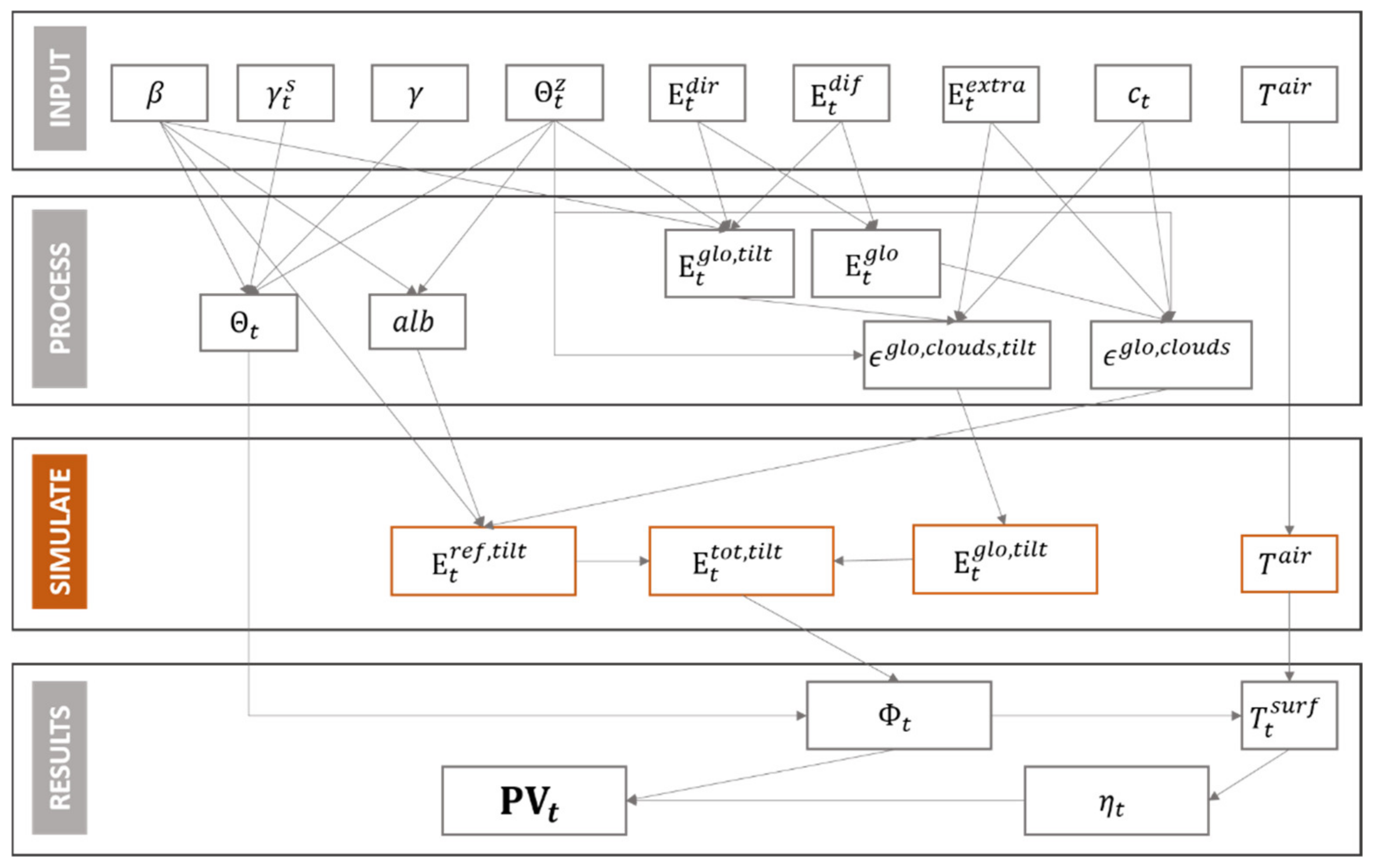
2.1. Solar Power Production Modeling

Here, we introduce the relevant basics of solar power production. For an overview of how all the variables below are connected, please refer to Figure A1 in Appendix A. The output of electric power generated by a photovoltaic panel at time instance t, P V t , is given by
P V t = Φ t η t
with η t being the photovoltaic or solar panel’s efficiency and Φ t   the solar flux. Thereby, η t is time-dependent, as it is influenced by the panels’ surface temperature T e m p t s u r f . It can be modeled by a linear relationship between both variables [20,21]. In most cases, the relationship between η t and T e m p t s u r f is derived from the respective photovoltaic panel data sheets [22,23]. For the modules produced by the German company SolarEdge, η t = 18.9 100 % 0.4 % / T e m p t s u r f 25   . The surface temperature T e m p t s u r f is calculated via the total solar irradiation E t t o t   received by the photovoltaic system’s surface of size A S with an incidence angle Θ t at hour t:
T e m p t s u r f = T e m p t a i r + 0.03   m 2 W h E t t o t
where T e m p t a i r denotes the average air temperature. The solar flux Φ t is defined as
Φ t = E t t o t A S cos Θ t .
The incidence angle Θ t can be calculated (R package solaR) using information about the movements of earth and sun as follows [24]
Θ t = arccos ( cos Θ t Z cos β + sin Θ t Z sin β cos γ t S γ ) ,
where β denotes the panel’s tilt, Θ t Z   the solar zenith angle at that specific time, γ t S the corresponding sun’s azimuth angle, and γ the panel’s azimuth. Note that Θ t is also a zenith angle. The solar position algorithm of Michalsky [24] allows calculating all these values with a maximum error of ±0.01° in both solar zenith and azimuth angle [25], which is accurate enough for the application used in this work. This algorithm also calculates the extraterrestrial irradiation E t e x t r a .
For horizontally arranged solar panels, E t t o t equals the global irradiation at time t, E t g l o , which is the sum of the direct irradiation E t d i r and indirect or diffuse irradiation E t d i r . Thereby, E t d i r can be calculated based on E t g l o [24], and E t d i f = E t g l o E t d i r consequently. For tilted solar panels, we have to add reflected irradiation E t r e f g . Additionally, E t d i r and E t d i f are slightly changed to direct and diffuse irradiation on the tilted ground, noted by E t d i r , t i l t , E t d i f , t i l t [26]. We can compute direct, diffuse, and reflected irradiation on the tilted ground using the Albedo a l b ( Θ t Z ) , which estimates how much irradiation is reflected from a surface (see Equation (6)). According to Alboteanu et al. [27], the formulas read
E t d i r , t i l t = E t d i r cos Θ t cos Θ t Z , E t d i f , t i l t = E t d i f 1 2 ( 1 + cos β ) , E t r e f , t i l t = E t g l o a l b Θ t Z 2 ( 1 cos β ) .
The Albedo is exponentially increasing with a decreasing declination of the sun: the higher Θ t Z , the more light is reflected from the ground surrounding the panels. As it is difficult to obtain a functional form for the Albedo, we have to use approximations. We assume that the photovoltaic panels are mounted on roofs; hence, we assume an Albedo of 20% if the sun’s declination is above a certain boundary [28]. Below this boundary, we approximate the Albedo using a linear function a l b ( Θ t Z ) :
a l b ( Θ t Z ) = 20 % 100 % 8 / 3 90 ° Θ t Z % °                       i f   Θ t Z 60 ° e l s e .

2.2. How to Incorporate Clouds into the Model

The model of Bird and Hulstrom [7] (assuming clear sky conditions) allows computing solar irradiation on horizontal surfaces with an accuracy of ±5%, while only basic atmospheric data are required. However, cloudy days are a lot more challenging to model. Myers [6] expands this model to the already mentioned CSM, where the relationship between irradiation under clear and under the cloudy sky is modeled via a multiplicative transmittance factor. Here, we propose a slight modification of this idea. We introduce two multiplicative factors, namely ϵ g l o   and ϵ g l o , t i l t ,   one for the global irradiation on the plain ground (to compute the Albedo influence) and one for the global irradiation tilted ground. The factors are used to establish a connection between extraterrestrial irradiation E t e x t r a and irradiation on the ground under tilted conditions at time t:
E t g l o , c l o u d s = E t e x t r a ϵ g l o , E t g l o , t i l t , c l o u d s = E t e x t r a ϵ g l o , t i l t .
Using Equation (7), we can replace the first two formulas in Equation (5). The reflected irradiation under cloudy conditions, again, is computed using E t g l o , c l o u d s from Equation (7) and the Albedo function (6) in Equation (5). Eventually, we yield E t t o t under cloudy conditions as the sum of E t g l o , t i l t , c l o u d s and E t r e f , t i l t   under cloudy conditions. Via Equations (1)–(3), the power output P V t is eventually computed.

3. Modeling Temperature and Cloudiness

Given the model design above, a stochastic model for temperature, cloudiness, and global (tilted) irradiation is needed to simulate solar power production scenarios. Temperature is a significant driver, as it influences the solar panels’ efficiency. For this purpose, literature offers various so-called weather generators, which are models (mostly with corresponding software packages) that allow simulating different weather conditions [29]. As an alternative, a Fourier transform-based model is proposed [30]. More advanced (multivariate) approaches have one thing in common [31,32,33]: They contain a term that explicitly models the seasonal component. Most are autoregressive approaches, which is reasonable as the temperature will not change too much from one hour to the next. In most cases, a Gaussian distributed noise term is applied to include stochastic elements. The advantage of the autoregressive models is evident: They are easy to understand and handle, which is beneficial in practical application. Hence, we apply such a model to describe and simulate air temperature T e m p t a i r . A sine function captures the trend. Using the Fourier transform delivers slightly better results but adds complexity to the model. Moreover, it is usual to compute the daily average temperature using a sine or cosine-based formula in business. Accordingly, let S t be the annual seasonality on an hourly basis defined as
S t = a + b sin t c 2 π 365.25 24 ,
where t denotes the hourly time index and a , b , c are parameters to shift and scale the seasonal trend. To consider leap years, we write 365.25 instead of 365. The discrete-time hourly air temperature model itself is defined as
Δ T e m p t a i r = κ 1 S t T e m p t a i r Δ t + κ 2 S t 1 T e m p t 1 a i r Δ t + κ 3 S t 24 T e m p t 24 a i r Δ t + σ ϵ t ,
where κ 1 , κ 2 , κ 3 , ϵ t ∼ N(0, 1), and σ > 0 denotes the volatility. If desired, one could design volatility to be time-varying, i.e., σ is replaced by σ t (for potential models, refer to McNeil et al. [34]). The model itself is constructed to be mean-reverting around the annual seasonality S t , which is reasonable, as there might be warm and cold winters, but the average temperature in December is lower than in July. Additionally, we have an autoregression lag of 1 and 24. Lag 1 accounts that temperature usually is not significantly changing from one hour to the other, and Lag 24 is the daily seasonality. This seasonality is sometimes more robust and sometimes weaker (in case of temperature drops, for example), but it is there. On average, it is warmer at noon than at midnight. The larger κ 3 , the larger the effect of daily seasonality.
Cloudiness, again, is measured in Germany as discrete states between 0 (clear sky) and 8 (a dense blanket of clouds). In other countries, it is recorded in the percentage of sky covered. Cloud movement is very complicated to model, and as it is not the paper’s focus, we use a rather hands-on, data-driven approach. As distribution for the cloudiness, we propose using a conditional multinomial distribution conditional on the previous state to account for autoregressive effects. The transition probabilities are estimated based on a data set of measured cloudiness. Let c t C be the cloudiness at a specific hour and let C = c 1 , c 2 , , c k ,   k denotes the set of possible states of cloudiness. The conditional probability p i , j = P ( c t = c i c t 1 = c j ) of having a cloudiness level of c t = c i given that the cloudiness of the previous hour was c t 1 = c j is estimated as follows
p i , j = # d a y s   w i t h   c l o u d i n e s s   c i   g i v e n   c j   o n   t h e   p r e v i o u s   d a y # d a y s   w h e r e   p r e v i o u s   d a y   h a d   a   c l o u d i n e s s   o f   c j .
The result is a matrix of transition probabilities, making it very easy to simulate future cloud coverages.
The transmittance factors ϵ g l o , c l o u d s and ϵ g l o , t i l t , c l o u d s   from Equation (7) are modeled as linear functions depending on T t a i r , c t , incident angle Θ t Z , the current hour, and E e x t r a . A seasonality parameter is also included. For each hour, we fit the model
y t = α 0 + α 1 T e m p t a i r + α 2 c t + α 3 E t e x t r a + α 4 90 ° Θ t Z + s e a s o n t + γ t
using least squares estimation. Thereby, α 0 , α 1 , α 2 , α 3 , α 4 represent the linear coefficients, γ t N 0 ,   σ 2 the residuals, and y t is either ϵ t g l o , c l o u d s or ϵ t g l o , t i l t , c l o u d s . Moreover, s e a s o n t = cos m o n t h t   2 p i / 12 , whereby m o n t h t denotes the current month in numbers, i.e., March = 3. Note that we only obtain estimates for positive values of 90 ° Θ t Z , i.e., when the sun is above the horizon. For the calibration, historical values are used to obtain E t g l o , t i l t , c l o u d s via (7). As mentioned above, E t e x t r a can be computed according to Michalsky [24]. Mind that the parameter estimates of Equation (11) vary with β   and the azimuth choice. Hence, for each panel position, a new calibration is required.

4. Application to Real-World Solar Irradiation Data

For a summary of the simulation procedure, please refer to the flow chart in Figure A2 in Appendix A. Here—because it is the novel aspect of our model, and in order to keep the article short—we solely discuss the irradiation model. Given proper irradiation simulations, corresponding photovoltaic simulations can be derived as described in the flow chart (Figure A2).

4.1. Data

We use the Climate Data Center provided by the German Climate Service www.dwd.de (accessed on 1 February 2021) [35] for retrieving temperature and cloud coverage data. Irradiation data come from the CAMS Radiation Service v3.2 all-sky irradiation provided by MINES ParisTech, Paris, France. The acronym CAMS stands for Copernicus Atmosphere Monitoring Service, which provides data at a resolution of about 3 km–max. 5 km [36]. All data were accessed via www.soda-pro.com on 1 February 2021 [37]. An overview of the data sets, including length and sources, is given in Table 1.
In Figure 1, we exemplary plot one year (2018) of global solar radiation. We can see the expected seasonal swing and some substantial variation, making prediction quite hard and requiring the development of various scenarios to assess a financial investment influenced by irradiation values.
The daily pattern can only be conjectured; hence, we plot the patterns in two sample months in Figure 2. Now, the daily structure and the weather-related variation can be observed. There is a distinct daily seasonality; its extent is not constant and influenced by various weather phenomena. Figure 3, again, presents temperature and cloud cover data for 2018. The stochastic pattern of the cloud cover is observed. Temperature shows the expected characteristic annual swing with a significant drop in the first quarter of 2018 and some significant variation over the year. There is also some daily seasonality, which is not constant due to changing weather and events such as sudden temperature drops. A stochastic model needs to incorporate all those observations.

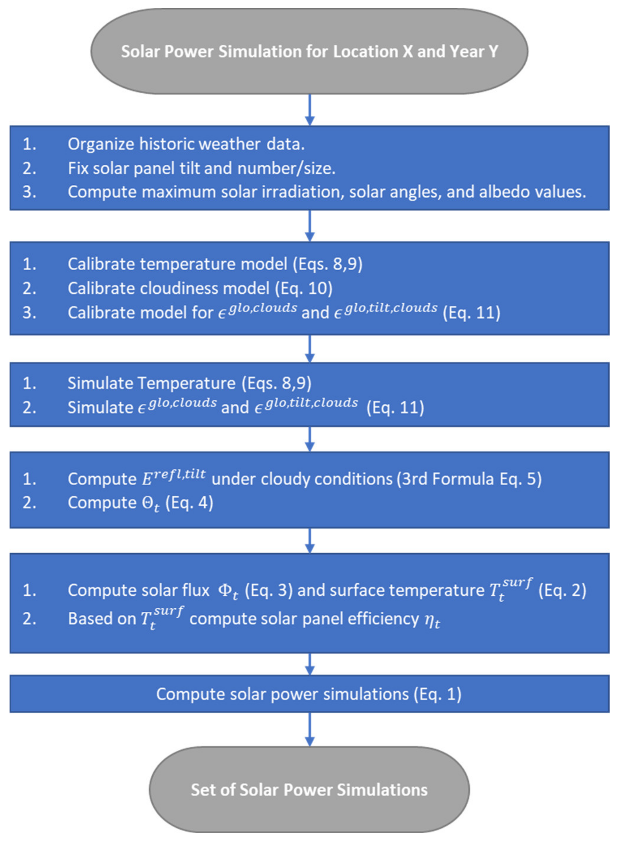
4.2. Model Calibration and Results

We calibrate the model from Equation (9) to the above data using nonlinear least-squares estimation to generate temperature simulations. This model includes both an annual and a daily seasonality and allows for enough variation to simulate temperature drops or unusually low or high temperatures. Again, transition probabilities for the cloud coverage are computed using the available data sets according to Equation (10). For detailed results, please refer to Table A1 in Appendix A. The transmittance coefficients are computed using Equation (11) calibrated to the given data sets. Parameter estimates are given in Table A2 and Table A3 in Appendix A.
In Figure 4, we exemplarily plot modeled hourly irradiation data for 2018 compared to the true values. It is not a simulated set but a descriptive model’s output. It shows that the model captures the annual swing, and values are in the range of the historical observations. On a first glimpse, our model looks a bit spikier. However, this might also be due to the resolution. In Figure 5, we show the results for February (as a winter month) and July (as a summer month) in detail. Note that values are computed for photovoltaic panels with a 30° southward tilt. We can see that the relevant dynamics are captured in both months, whereby our model produces a smoother version, which is due to the least-squares fitting of the model parameters in Equation (11). This is distinctly visible in the February data, where the model generates a smoothed version of reality.
Differences in the summertime are comparably lower than differences in wintertime, which is significant for assessing our model. In the summertime, irradiation values are higher, so we have more resulting photovoltaic power. Smaller model errors mean that simulations reflect better the true conditions in these months; hence, we can consider them more reliable. Considering the February data, we see that we underestimate irradiation values on days with comparably intensive sunshine. This might be due to an underestimation of reflexive irradiation due to snow, for example.

5. Quality Control and Discussion

5.1. Quality Control

For evaluating the quality of our model, we have to rely on assessing the irradiation values due to the lack of accurate historic photovoltaic data. This case study’s central and relevant findings can be summarized as follows: The annual errors’ average is approximately zero. Hence, the model is unbiased, and the annual sum of irradiation from the model is roughly equal to the historical measurements. Even if the hourly estimates are incorrect, the overall simulated irradiation is correct, and any financial analysis will not be biased. However, in this section, we want to look at model errors to understand the model better and know how to interpret and treat the resulting simulations.
On a monthly level, relative differences between the modeled and true irradiation amounts are maximum around plus/minus 8%, as shown in Figure 6. Consequently, given unbiased temperature simulation, we slightly overestimate photovoltaic power amounts in March and underestimate them in August. The rest of the months, especially May and December, show comparably smaller relative differences.
Eventually, we consider hourly data and compute (a) the relative standard errors (RSE), i.e., the differences’ standard deviation divided by the respective hourly mean, as well as (b) the median absolute percentage error (MAPE). The second measure is computed by including values from the data set at a particular hour and month. For example, we analyze the error for Hour 5 in January. The same is done for the MAPE. We compute errors for irradiation on plain and on the tilted ground in order to see whether this has an effect on the error levels.
Given a data set of T observations, it is defined for E t g l o as
M A P E E ^ t g l o t = 1 , , T , E t g l o t = 1 , , T , h o u r , m o n t h = 1 T j = 1 J E ^ j g l o E j g l o E j g l o ,
Thereby, E ^ j g l o denotes the estimated irradiation value at time instance j, whereby only values at a chosen hour and in a specific month are considered. Consequently, J denotes the length of this subset. The MAPE for E t g l o , t i l t   is computed analogously. Thereby, as above, we assume a 30° southward tilt. We compute the median, not the mean, as the standard definition of the MAPE implies. When looking at the errors’ distribution, we see a strong asymmetry as it is tilted to the right. Hence, the median is better to estimate the average absolute percentage error. Results for the average over hourly errors in monthly granularity for E t g l o and E t g l o , t i l t are given in Table 2.
The first thing we see is that errors indeed increase when considering E g l o , t i l t instead of E g l o . Additionally, we see that error measures are higher in the winter months than during summer. This is because irradiation values are higher during summer. Hence, the least squares optimization focuses more on those values than on the comparably lower values in winter. RSE values range between 25% and about 39% for E g l o and between 24% and 50% for E g l o , t i l t , whereby the highest values are observed between October and February, where absolute values are lowest over the year. Average MAPE values for E g l o range between 17% and 34% with the same annual pattern, i.e., showing higher values during winter. MAPE values for E g l o , t i l t are slightly higher, ranging between 18% and 43%. Therefore, it is reasonable that both MAPE and RSE values are higher for E g l o , t i l t   due to the higher proportion of direct irradiation, which is more complex to model than diffuse irradiation as it is more stochastic.
In order to understand the error levels summarized in Table 2, we have a closer look at the data. First, one has to consider that incidence angle, cloud coverage, temperature, and a parameter for the annual seasonality can only partly explain irradiation. In Figure 7, we plot irradiation versus cloud coverage. On the first day, the interdependencies are obvious as high cloudiness induces comparably low irradiation. On 5 and 6 February, global irradiation evolves constantly along with the daylight pattern, but cloudiness is oscillating significantly. However, when fitting Equation (10), the respective parameter α 2 is significant. One assumption is that hourly granularity already has too much aggregation and that temporary sunny periods within an hour overcompensate the cloudy phases. Additionally, global irradiation also considers indirect irradiation, which contributes to the total value also in clouded phases. Above that, there might be other influence factors or nonlinear interdependencies that have not been considered yet. However, the latter would mean the reliance on even more data, where the current data sets are sometimes hard to obtain. Working, for example, with 10-min data increases the amount of data by a factor 6. Moreover, data quality on an hourly level is comparably higher.

5.2. Discussion

For evaluating the potential of our model, we have to consider alternatives as well. Note that literature exclusively focuses on horizontal values, which is reasonable as tilt offers too much variety.
Politaki and Alouf’s model [14] is thereby the model closest to our approach. Their model is based on the Clear Sky Model of Bird and Hulstrom [7], which is extended by a multiplicative stochastic factor to (a) include cloudiness and (b) allow for simulating irradiation values. However, it is hard to compare their model to ours regarding error numbers, as they show only root mean squared errors, which are even aggregated to an annual level. Given the strong seasonality of irradiation values, this information is only of limited value. Additionally, there is one significant drawback: as it is based on the Clear Sky Model, we require additional data such as pressure and aerosol depth. Especially the latter is hard to obtain—even more if historical observations are required. Lockart et al. [38] state that their simulation models achieve preciseness of 8%. However, they consider daily values and ignore intraday patterns, which are the challenging part here. Anand et al. [39] focus on the distributional properties. Trend and seasonal aspects are captured via a symmetric moving average given historical observations and then filtered. After that, first-order differences eliminate the last deterministic information. Simulation is purely done via the distribution fitted to the residuals of the previously described process. The advantage of their idea is that only historic irradiation values are required; however, limiting the annual and daily swing to a fixed average value narrows the range of possible scenarios significantly. Extraordinarily long/short summers or comparably cold/warm winters cannot be modeled in their setup. As we simulate temperature separately, our model accounts for different weather scenarios.
Benth et al. [9] use the sun intensity to identify and eliminate the seasonal component’s influence. Afterward, they fit an autoregressive process, which can also be used for simulation purposes. Here, no local but regionally aggregated data on a daily level are used. Hence, this is also not an alternative to our approach.
These few examples illustrate that, despite a wide range of literature about this topic, it is hard to compare individual models. These vary in granularity (hourly, daily) and objective. However, we can state a few things. Compared to existing approaches which are close to our model [6,7], we can significantly reduce the amount of climate data required for calibration at the cost of reduced accuracy. One does not have to consider factors such as water vapor, ozone level, aerosol optical depth, and air pressure. These influence factors are all time-varying, and historical measurements (for model calibration purposes) are hard to obtain. Our model is much more user-friendly, as it is easier to handle and calibrate. Hourly error levels seem to be high at first sight. However, solar irradiation is a highly complex physical parameter. Moreover, our intention is not to model but to simulate data. Error values are also given to see whether numbers increase in the case of tilted irradiation. More importantly, the model is unbiased on an annual level, and model bias on a monthly level is relatively low.

6. Conclusions

Simulating photovoltaic power is required in the energy risk management of power utilities, power plant operators, and energy trading companies. Because of the relevance of this topic, literature already offers methods and tools to simulate photovoltaic power. This article adds a new parametric model to simulate solar irradiation and, consequently, photovoltaic power on an hourly level. Our approach is based on the idea that simulated global irradiation values are scaled values of extraterrestrial irradiation. The (hourly) scaling factors are obtained via linear functions that include factors such as temperature, cloudiness, or maximum possible irradiation. An annual trend is included as well. In order to derive corresponding solar power values, we integrate our approach into the cloudy sky model designed by Myers [6]. Our results are positive: the simulated irradiation pattern is similar to historical data. Additionally, we see no bias in the total solar power output compared to the previous years. We have a clear and straightforward approach that includes the interdependencies between the individual weather factors. Hence, different possible weather scenarios are covered, but no complex physical knowledge or considerable computational power is needed. The application is therefore also suitable for optimizing the operation of isolated photovoltaic grids.
However, from a modeling point of view, there is still some research to be done in the future. Relative errors of solar irradiation models are relatively high compared to other fields of application. Especially in the wintertime, our model lacks some precision. Future research needs to verify whether nonlinear models should be considered as well or whether other weather factors such as precipitation and aerosol density should be included.

Author Contributions

Conceptualization, S.S. and F.M.; methodology, S.S., F.M. and M.K.; software, S.S.; validation, S.S., F.M. and M.K.; investigation, S.S., F.M., M.K., P.M. and A.H.; resources, S.S.; data curation, S.S. and F.M.; writing, S.S., F.M., M.K., P.M. and A.H.; visualization, S.S. and F.M.; supervision, S.S. and P.M. All authors have read and agreed to the published version of the manuscript.

Funding

This research has been funded by the Ministry of Education, Science, and Technological Development of the Republic of Serbia. The article processing charge was funded by the Baden-Wuerttemberg Ministry of Science, Research and Culture and Ulm University of Applied Sciences in the funding program Open Access Publishing.

Institutional Review Board Statement

Not applicable.

Informed Consent Statement

Not applicable.

Data Availability Statement

Not applicable.

Conflicts of Interest

The authors declare no conflict of interest. The funders had no role in the design of the study; in the collection, analyses, or interpretation of data; in the writing of the manuscript, or in the decision to publish the results.

Appendix A

Figure A1. Parameter interactions.
Sustainability 14 04617 g0a1
Figure A2. Flow chart of the proposed solar irradiation model.
Sustainability 14 04617 g0a2
Table A1. Cloud coverage transition matrix for Ulm, Germany.
From/To012345678
068.93%7.95%4.70%3.41%2.78%2.58%2.45%4.26%2.94%
131.02%12.98%9.95%7.90%8.29%7.51%4.98%9.27%8.10%
218.11%11.19%12.31%10.99%8.95%10.27%7.53%11.50%9.16%
312.40%7.66%9.66%9.66%12.31%11.58%9.39%16.13%11.21%
48.62%6.81%7.80%10.92%12.56%13.63%12.64%15.68%11.33%
56.38%4.77%7.18%9.09%11.22%12.46%12.10%20.09%16.72%
64.36%3.37%6.20%7.66%9.64%10.03%13.14%26.67%18.94%
71.99%1.82%1.60%2.73%3.08%4.14%6.34%32.27%46.03%
80.58%0.46%0.47%0.65%0.80%1.06%1.38%14.44%80.16%
Table A2. Parameters for estimating E g l o of Ulm.
HourIntercept c t 90 ° Θ z E e x t r a T a i r Seasonality
60.8664−0.0447−0.10850.00410.00520.0565
70.9336−0.0466−0.15560.00610.00380.1519
81.1537−0.0460−0.02510.00020.00440.2764
91.1165−0.0449−0.0077−0.00030.00610.2492
100.8488−0.0423−0.03560.00140.00600.1797
110.7877−0.0377−0.02300.00090.00830.1552
120.7460−0.0325−0.01970.00080.00820.1694
130.7132−0.0306−0.01540.00060.00780.1571
140.6043−0.0285−0.01890.00080.00710.1300
150.5085−0.0232−0.02190.00090.00620.1297
160.2547−0.0184−0.06540.00310.00420.1147
170.0964−0.0134−0.01410.00100.00200.0379
180.0256−0.0084−0.01800.00130.00080.0592
19−0.0276−0.0044−0.02010.0015−0.00050.0320
Table A3. Parameters for estimating E g l o , t i l t of Ulm.
HourIntercept c t 90 ° Θ z E e x t r a T a i r Seasonality
60.39300.0063−0.20510.0089−0.0011−0.1730
70.8892−0.0336−0.05590.00170.00070.0954
80.9814−0.0427−0.04370.00130.00440.1819
91.0066−0.0452−0.04230.00140.00600.2181
100.7323−0.0451−0.05830.00270.00600.1548
110.7920−0.0403−0.04140.00180.01170.1808
120.9114−0.0354−0.03320.00120.01300.2369
130.9308−0.0398−0.02670.00090.01190.1983
140.8582−0.0449−0.03340.00130.01060.1491
150.6622−0.0401−0.04850.00210.00780.1243
160.2767−0.0271−0.10580.00500.00450.0870
170.1091−0.0173−0.12300.00580.00180.0498
180.01606−0.0060−0.01040.00090.00050.0273
19−0.02800.0007−0.00970.0009−0.00070.0174

References

  1. Mitić, P.; Kostić, A.; Petrović, E.; Cvetanović, S. The Relationship between CO2 Emissions, Industry, Services and Gross Fixed Capital Formation in the Balkan Countries. Eng. Econ. 2020, 31, 425–436. [Google Scholar] [CrossRef]
  2. Li, D.; Yang, D. Does Non-Fossil Energy Usage Lower CO2 Emissions? Empirical Evidence from China. Sustainability 2016, 8, 874. [Google Scholar] [CrossRef] [Green Version]
  3. Petrović-Ranđelović, M.; Mitić, P.; Zdravković, A.; Cvetanović, D.; Cvetanović, S. Economic growth and carbon emissions: Evidence from CIVETS countries. Appl. Econ. 2020, 52, 1806–1815. [Google Scholar] [CrossRef]
  4. Voyant, C.; Notton, G.; Kalogirou, S.; Nivet, M.L.; Paoli, C.; Motte, F.; Fouilloy, A. Machine learning methods for solar radiation forecasting: A review. Renew. Energy 2017, 105, 569–582. [Google Scholar] [CrossRef]
  5. Zhang, J.; Zhao, L.; Deng, S.; Xu, W.; Zhang, Y. A critical review of the models used to estimate solar radiation. Renew. Sust. Energy Rev. 2017, 70, 314–329. [Google Scholar] [CrossRef]
  6. Myers, D.R. Cloudy Sky Version of Bird’s Broadband Hourly Clear Sky Model. NREL Technical Report. In Proceedings of the SOLAR 2006 “Renewable Energy: Key to Climate Recovery”, Denver, CO, USA, 8–13 July 2006; Available online: https://www.nrel.gov/docs/fy06osti/40115.pdf (accessed on 7 February 2022).
  7. Bird, R.E.; Hulstrom, R.L. Simplified Clear Sky Model for Direct and Diffuse Insolation on Horizontal Surfaces (No. SERI/TR-642-761); Solar Energy Research Institute: Golden, CO, USA, 1981. Available online: https://www.nrel.gov/docs/legosti/old/761.pdf (accessed on 7 February 2022).
  8. Jasmin, B.; Taheri, P. An Origami-Based Portable Solar Pael System. In Proceedings of the 2018 IEEE 9th Annual Information Technology, Electronics and Mobile Communication Conference, Vancouver, BC, Canada, 1–3 November 2018. [Google Scholar]
  9. Benth, F.E.; Ibrahim, N. Stochastic Modelling of Photovoltaic Power Generation and Electricity Prices. J. Energy Mark. 2017, 10, 275–309. [Google Scholar] [CrossRef]
  10. Dong, J.; Olama, M.M.; Kuruganti, T.; Melin, A.M.; Djouadi, S.M.; Zhang, Y.; Xue, Y. Novel stochastic methods to predict short-term solar radiation and photovoltaic power. Renew. Energy 2020, 145, 333–346. [Google Scholar] [CrossRef]
  11. Abdel-Nasser, M.; Karar, M. Accurate photovoltaic power forecasting models using deep LSTM-RNN. Neural Comput. Appl. 2019, 31, 2727–2740. [Google Scholar] [CrossRef]
  12. Miozzo, M.; Zordan, D.; Dini, P.; Rossi, M. SolarStat: Modeling photovoltaic sources through stochastic Markov processes. In Proceedings of the 2014 IEEE International Energy Conference (ENERGYCON), Cavtat, Croatia, 13–16 May 2014. [Google Scholar] [CrossRef] [Green Version]
  13. Barukčić, M.; Hederić, Ž.; Hadžiselimović, M.; Seme, S. A simple stochastic method for modelling the uncertainty of photovotaic power production based on measured data. Energy 2018, 165, 246–256. [Google Scholar] [CrossRef]
  14. Politaki, D.; Alouf, S. Stochastic Models for Solar Power. In Computer Performance Engineering. EPEW 2017. Lecture Notes in Computer Science; Reinecke, P., Di Marco, A., Eds.; Springer: Cham, Switzerland, 2017; Volume 10497, pp. 282–297. [Google Scholar] [CrossRef] [Green Version]
  15. Gueymard, C.A. Parametrized transmittance model for direct beam and circumsolar spectral irradiance. Sol. Energy 2001, 71, 325–346. [Google Scholar] [CrossRef]
  16. Badescu, V.; Gueymard, C.A.; Cheval, S.; Oprea, C.; Baciu, M.; Dumitrescu, A.; Iacobescu, F.; Milos, I.; Rada, C. Accuracy analysis for fifty-four clear-sky solar radiation models using routine hourly global irradiance measurements in Romania. Renew. Energy 2013, 55, 85–103. [Google Scholar] [CrossRef]
  17. Ineichen, P. Validation of models that estimate the clear sky global and beam solar irradiance. Sol. Energy 2016, 132, 332–344. [Google Scholar] [CrossRef] [Green Version]
  18. Hofmann, M.; Seckmeyer, G. A New Model for Estimating the Diffuse Fraction of Solar Irradiance for Photovoltaic System Simulations. Energies 2017, 10, 248. [Google Scholar] [CrossRef] [Green Version]
  19. Khatib, T.; Mohamed, A.; Sopian, K. A review of solar energy modeling techniques. Renew. Sustain. Energy Rev. 2012, 16, 2864–2869. [Google Scholar] [CrossRef]
  20. Moharram, K.A.; Abd-Elhady, M.S.; Kandil, H.A.; El-Sherif, H. Enhancing the performance of photovoltaic panels by water cooling. Ain. Shams Eng. J. 2013, 4, 869–877. [Google Scholar] [CrossRef] [Green Version]
  21. Brecl, K.; Topič, M. Development of a Stochastic Hourly Solar Irradiation Model. Int. J. Photoenergy 2014, 2014, 376504. [Google Scholar] [CrossRef] [Green Version]
  22. SolarEdge. Available online: https://www.solaredge.com/sites/default/files/se-smart-modules-white-datasheet-aus.pdf (accessed on 7 February 2022).
  23. JinkoSolar. Available online: https://www.jinkosolar.com/uploads/CheetahPerc%20JKM325-345M-60H-(V)-A3-EN.pdf (accessed on 7 February 2022).
  24. Michalsky, J.J. The Astronomical Almanac’s algorithm for approximate solar position (1950–2050). Sol. Energy 1988, 40, 227–235. [Google Scholar] [CrossRef]
  25. Andreas, A.; Reda, I. Solar Position Algorithm for Solar Radiation Applications (Revised), Technical Report, NREL/TP-560-34302; National Renewable Energy Laboratory: Golden, CO, USA, 2008. Available online: https://www.nrel.gov/docs/fy08osti/34302.pdf (accessed on 7 February 2022).
  26. Duffie, J.A.; Beckman, W.A. Solar Engineering of Thermal Processes, 4th ed.; John Wiley & Sons, Inc.: Hoboken, NJ, USA, 2013; ISBN 978-047-087-366-3. [Google Scholar]
  27. Alboteanu, I.L.; Bulucea, C.A.; Degeratu, S. Estimating Solar Irradiation Absorbed by Photovoltaic Panels with Low Concentration Located in Craiova, Romania. Sustainability 2015, 7, 2644–2661. [Google Scholar] [CrossRef] [Green Version]
  28. Schönwiese, C.D. Klimatologie, 4th ed.; UTB GmbH: Stuttgart, Germany, 2013; ISBN 978-382-523-900-8. [Google Scholar]
  29. Richardson, C.W. Stochastic simulation of daily precipitation, temperature, and solar radiation. Water Resour. Res. 1981, 17, 182–190. [Google Scholar] [CrossRef]
  30. Campbell, G.S.; Norman, J.M.A. Introduction to Environmental Biophysics; Springer Science+Business Media: New York, NY, USA, 1998. [Google Scholar] [CrossRef]
  31. Parey, S. Generating a Set of Temperature Time Series Representative of Recent Past and Near Future Climate. Front. Environ. Sci. 2019, 7, 99. [Google Scholar] [CrossRef]
  32. Breinl, K.; Turkington, T.; Stowasser, M. Simulating daily precipitation and temperature: A weather generation framework for assessing hydrometeorological hazards. Meteorol. Appl. 2014, 22, 334–347. [Google Scholar] [CrossRef]
  33. Smith, K.; Strong, C.; Rassoul-Agha, F. A New Method for Generating Stochastic Simulations of Daily Air Temperature for Use in Weather Generators. J. Appl. Meteorol. Climatol. 2017, 56, 953–963. [Google Scholar] [CrossRef] [Green Version]
  34. McNeil, A.J.; Frey, R.; Embrechts, P. Quantitative Risk Management: Concepts, Techniques, and Tools—Revised Edition; Princeton University Press: Princeton, NJ, USA, 2015; ISBN 978-0-691-16627-8. [Google Scholar]
  35. Deutscher Wetterdienst. Available online: https://www.dwd.de (accessed on 7 February 2022).
  36. Global Modeling and Assimilation Office (GMAO). MERRA-2 tavg1 2d slv Nx: 2d,1-Hourly, Time-Averaged, Single-Level, Assimilation, Single-Level Diagnostics V5.12.4; Goddard Earth Sciences Data and Information Services Center (GES DISC): Greenbelt, MD, USA, 2015. [Google Scholar] [CrossRef]
  37. SoDa. Solar Radiation Data. Available online: https://www.soda-pro.com (accessed on 7 February 2022).
  38. Lockart, N.; Kavetski, D.; Franks, S.W. A New Stochastic Model for Simulating Daily Solar Radiation from Sunshine Hours. Int. J. Climatol. 2015, 35, 1090–1106. [Google Scholar] [CrossRef]
  39. Anand, M.P.; Rajapakse, A.; Bagen, B. Stoachstic Model for Generating Synthetic Hourly Global Horizontal Solar Radiation Data Sets Based on Auto Regression Characterization. Int. Energy J. 2020, 20, 181–200. [Google Scholar]
Figure 1. Hourly global solar irradiation from Ulm 2018.
Sustainability 14 04617 g001
Figure 2. Hourly global solar irradiation from Ulm in May and October 2018.
Sustainability 14 04617 g002
Figure 3. Hourly temperature and cloud cover data from Ulm in 2018.
Sustainability 14 04617 g003
Figure 4. Hourly irradiation data for 2018: our model vs. reality.
Sustainability 14 04617 g004
Figure 5. Real and simulated global tilted irradiation.
Sustainability 14 04617 g005aSustainability 14 04617 g005b
Figure 6. Relative difference between modeled and measured irradiation amounts (plain ground) on a monthly level for Ulm data between 2015 and 2018.
Sustainability 14 04617 g006
Figure 7. Global irradiation vs. cloudiness on a horizontal plane from 4 to 6 September 2014 in Ulm.
Sustainability 14 04617 g007
Table 1. Data sets (all accessed on 1 February 2021).
Data SetSourceFrom/ToLength
Temperature Ulmwww.dwd.de [35]1 January 2014–31 December 201837,924
Cloud Cover Ulmwww.dwd.de [35]1 January 2014–31 December 201837,381
Irradiation Ulmwww.soda-pro.com [37]1 January 2013–31 December 201852,584
Table 2. Errors of estimating global (tilted) irradiation in Ulm.
E g l o
JanuaryFebruaryMarchAprilMayJune
RSE37.82%38.94%29.71%29.17%27.97%25.11%
MAPE29.01%30.78%25.96%22.27%19.85%17.74%
JanuaryFebruaryMarchAprilMayJune
RSE25.66%27.50%29.65%34.96%38.74%32.06%
MAPE17.18%17.86%21.55%29.48%32.05%33.55%
E g l o , t i l t
JanuaryFebruaryMarchAprilMayJune
RSE49.98%47.76%37.57%27.50%29.15%24.19%
MAPE37.44%39.14%31.12%24.62%23.07%18.95%
JanuaryFebruaryMarchAprilMayJune
RSE25.37%27.49%31.86%43.92%48.80%49.33%
MAPE17.74%20.01%25.14%37.65%43.23%39.13%
Publisher’s Note: MDPI stays neutral with regard to jurisdictional claims in published maps and institutional affiliations.

