Abstract
Ecosystem service research is essential to identify the contribution of the ecosystem to human welfare. As an important ecological barrier zone, the Qinghai-Tibet Plateau (QTP) supports the use of a crucial wind erosion prevention service (WEPS) to improve the ecological environment quality. This study simulated the spatiotemporal patterns of the WEPS based on the Revised Wind Erosion Equation (RWEQ) and its driving factors. From 2000 to 2015, the total WEPS provided in the QTP ranged from 1.75 × 10⁹ kg to 2.52 × 10⁹ kg, showing an increasing and then decreasing trend. The average WEPS service per unit area was between 0.72 kg m−2 and 1.06 kg m−2. The high-value areas were concentrated in the northwest and north of the QTP, and the total WEPS in different areas varied significantly from year to year. The average retention rate of the WEPS in the QTP was estimated to be 57.24–62.10%, and high-value areas were mainly located in the southeast of the QTP. The total monetary value of the WEPS in the QTP was calculated to be between 223.56 × 10⁹ CNY and 321.73 × 10⁹ CNY, and the average WEPS per unit area was between 0.08 CNY m−2 and 0.13 CNY m−2, showing a declining–rising–declining trend. The high-value areas gradually expanded to the west and east of the QTP. The slope was the most important factor controlling the spatial differentiation of the WEPS, followed by the landform type, average annual precipitation, and average annual wind speed, and human activities such as land-use change could improve the WEPS by returning farmland to grassland and desertification control in the QTP.
1. Introduction
The Qinghai-Tibet Plateau (QTP) is the most unique geographical unit in the world because of its high altitude and mountainous landforms. The QTP is considered an important ecological barrier in south-western China, as it supports various ecosystem services in the region and in neighboring countries [1,2]. Among these ecosystem services, wind erosion prevention service (WEPS) is very important because of the extreme climate and low vegetation coverage in most parts of the plateau [3,4,5,6,7]. The average wind erosion rate for the plateau as a whole reached the medium erosion standard in 2001 [8], and the area of desertification in the QTP accounted for 15.1% of the total region in 2015 [9]. Therefore, it is critical to assess the regional WEPS and analyze the influencing factors in order to forecast wind erosion and provide a scientific basis for desertification control [10].
The WEPS can be estimated by the difference between potential and actual sand erosion by ecosystems. Several models have been adopted to simulate sand erosion by ecosystems, including the sediment transport equation [11], the wind erosion equation (WEQ) [12], the Texas erosion analysis model (TEAM) [13], the description model [14], the revised wind erosion equation (RWEQ) [15], the wind erosion prediction system [16], and the wind erosion stochastic simulator (WESS) [17]. Among these models, the RWEQ model is most commonly used for sand erosion simulations in the QTP. For example, Jiang [18] used the RWEQ model to evaluated wind erosion modules in Qinghai and showed that the total area of wind erosion in Qinghai Province accounts for more than half of the regional area, and the level of wind erosion damage in the Qaidam Basin is relatively serious. Huang [19] analyzed the WEPS of ecosystems in the Tibet Plateau from 1990 to 2010 by RWEQ, showing that the annual average soil wind erosion modulus, the average sand fixation service quantity, and the retention rate of the average annual WEPS in the Tibet Plateau were 1.58 kg m2, 18.99 × 10⁸ t, and 66.5%, respectively. Teng [10] adopted the RWEQ model to simulate the WEPS of the QTP from 2000 to 2015. However, studies on WEPS in this area have been limited, with most studies only involving local areas [20,21]. Accordingly, few studies have comprehensively described the WEPS and its dynamic characteristics over the whole QTP. As the terrain of the QTP is complex, the spatial pattern of sand erosion and WEPS may differ significantly between the east and west parts [9]. Few studies have examined wind erosion throughout the QTP or investigated the changes among different areas and ecosystems.
In recent years, many scholars have used multi-source data and methods such as the linear correlation model, multiple regression model, structural equation model, and constraint effect to investigate the factors (vegetation coverage, wind speed, precipitation, animal husbandry development, land use, etc.) driving the WEPS [10,22,23,24,25,26,27]. Latocha et al. showed that changes in land use have affected soil erosion to a larger extent than climate change in the Sudetes Mts. within the last 150 years [28]. Garbrecht et al. showed that warmer temperatures and reduced rainfall could exacerbate soil wind erosion in farmland areas in the southern Great Plains [29]. Li argued that the increase in the afforestation area is the main factor driving the improvement of WEPS in Inner Mongolia [30]. Sharratt showed that increase in the crop yield in the Colombian Plateau could reduce damage from soil wind erosion [31]. Few studies have conducted a driving factor analysis of the WEPS in the QTP. Teng [10] simulated the influences of climate changes and human activities on sand erosion and the WEPS in the QTP from 2000 to 2015 through comparative analysis of spatiotemporal dynamics. The above studies have helped us to understand the driving mechanism responsible for the spatial distribution pattern of WEPS, but there are still gaps in our knowledge on the interaction of different driving factors.
The geographic detector is a spatial statistical method based on spatial differentiation that is used to reveal the driving mechanism of a variable [32]. The geographic detector can analyze the interaction between two independent variables and determine the specific effect type while detecting the influences of variables with attributes of different types and values on the spatial distribution of the dependent variable. At present, the geographic detector is widely used in the analysis of the change process of spatial patterns in many fields such as meteorology, environmental pollution, ecology, human health, and regional planning [33,34,35,36,37,38,39]. Few studies have adopted the geographic detector to analyze the driving factors related to the WEPS. Zhang [40] conducted an exploratory study on the factors driving changes in the WEPS in Xilingol League using the geographic detector, and proved that the application of the geo-detector analysis on the WEPS is rational and scientific. The application of geographic detectors to analyze the factors driving changes in the spatial pattern of WEPS can account for the influences of type variables and numerical variables on service changes, analyze the interactions between various factors, and make up for the lack of analysis of factors driving the spatial distribution of the WEPS.
Therefore, this study adopted the RWEQ model to simulate the WEPS in the QTP from 2000 to 2015, estimated its monetary value using the restoration cost method, evaluated the differences in the material and monetary value of the WEPS among different cities and ecosystems, and analyzed the contributions and interactions of natural and human factors in the formation and evolution of the spatial pattern of the WEPS. This study can be used to improve the understanding of the spatial patterns of the WEPS in the QTP and provides crucial knowledge that can be used to make decisions about ecological restoration and protection to improve the WEPS in different ecosystems.
2. Methodology and Data
2.1. Study Area
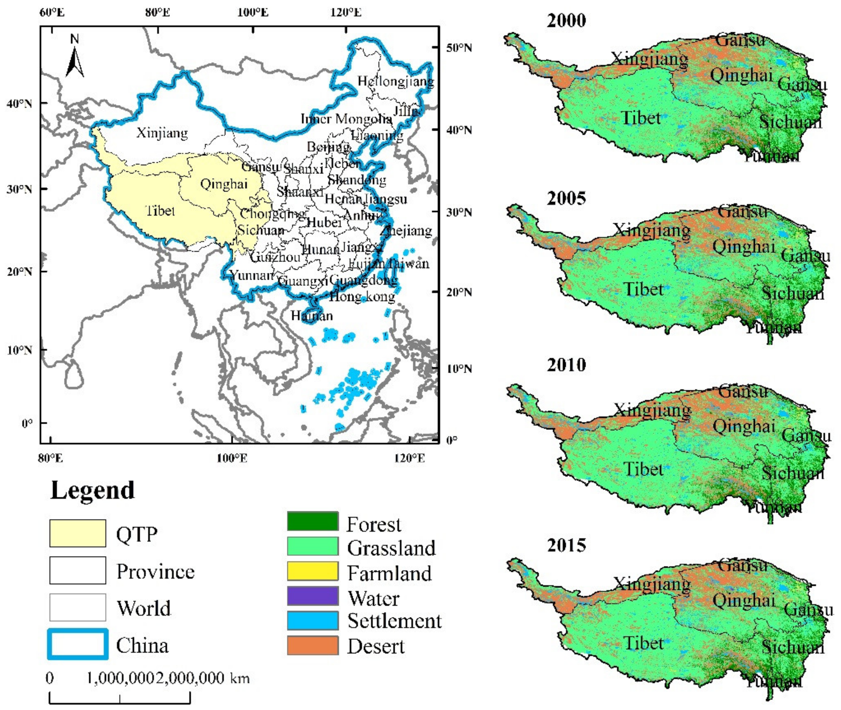
The QTP is located in southwestern China, and involves five provinces (autonomous regions): Qinghai, Tibet, Sichuan, Xinjiang, Gansu, and Yunnan (Figure 1). In the western part of the QTP is the Pamir Plateau and the Karakoram Mountains, bordering Tajikistan and Pakistan, and in the southern part there are the Himalayas, bordering Nepal, Bhutan, and other countries. The QTP has an average elevation of more than 4000 m. The highest altitude is found on Mount Everest, 8844.43 m, whereas the Jinsha River is only 1503 m above sea level. The special geographical location of the QTP means that it has a unique plateau climate with a cold, hypoxic, and arid climate with strong radiation. The temperature is 15–20 °C lower than that of other areas at the same latitude. The complex terrain in this area also causes the climate to vary. The temperature decreases from southeast to northwest, and the average annual temperature can reach below −6 °C. Due to the blocking effect of the multiple high mountains, the annual precipitation decreases from south to north, and the annual precipitation is less than 50 mm. The total annual solar radiation on the QTP can be as high as 5400–7900 MJ·m−2·year−1, and the total annual sunshine hours are 2500–3200 h.
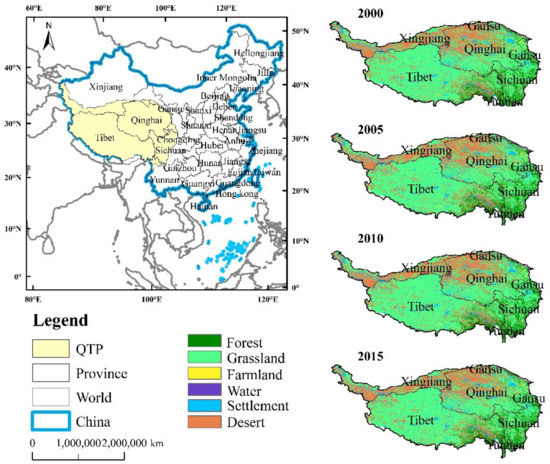
Figure 1.
Location of the Qinghai-Tibet Plateau (QTP) and the land cover map from 2000 to 2015.
2.2. Method and Data
2.2.1. Calculation of WEPS
The WEPS represents the reduction of wind erosion caused by vegetation and is calculated as the difference between the potential wind erosion under bare soil conditions and the actual wind erosion under vegetation conditions. The potential and actual wind erosion are calculated with the RWEQ model [15,41]. The actual wind erosion is the level of soil erosion under the condition of vegetation coverage in a real scenario, whereas the potential wind erosion is the level of soil erosion under bare land conditions without vegetation. The WEPS was calculated as follows:
where SLR represents the potential wind erosion (kg m−2); Qrmax represents the maximum potential sediment transport capacity (kg m−1); Sr represents the potential critical plot length (m); SL represents the actual wind erosion (kg m−2); Qmax represents the maximum sediment transport capacity (kg m−1); S represents the critical plot length (m); G represents the WEPS (kg m−2); z represents the calculated downwind distance (m); and WF, EF, SCF, K′, and C correspond to the factors of weather (kg m−1), the soil erodibility fraction (%), soil crust factor (dimensionless), the soil roughness factor (dimensionless), and vegetation (dimensionless), respectively. The WF was calculated as follows:
where Wf is the wind factor (m3 s−1); g represents the gravitational acceleration (m2 s−1); ρ represents the air density (kg m−3); SW is the soil moisture factor (dimensionless); and SD represents the snow cover factor (dimensionless), which is the ratio of days with no snow cover to the total number of days studied. A snow cover depth less than 25.4 mm indicates no snow cover. The expression u1 represents the threshold wind velocity at a height of 2 m (m s−1). The threshold wind velocity for sand lands and sandy grasslands is 5 m s−1; u2 represents the monthly average wind velocity at a height of 2 m (m s−1); and Nd represents the number of days with a monthly average wind velocity that exceeds the threshold wind velocity.
In this study, EF and SCF were assumed to be unchanged over time and were calculated using the soil raster data that were converted from a 1:1,000,000 soil data shapefile provided by the Harmonized World Soil Database (HWSD) developed by the International Institute for Applied System Analysis (IIASA) of the FAO. For the calculation, the classification criteria for soil texture taken from international data in the database were converted to American criteria to meet the factor calculation requirements by using the logistic growth model proposed by Skaggs et al. [42]. The values of EF and SCF were calculated as follows:
where Sa, Si, Cl, OM, and CaCO3 represent the content of sand, silt, clay, organic matter, and calcium carbonate (%), respectively.
The value of K′ was calculated with the following equation:
where α represents the slope gradient and was calculated by a digital elevation model (DEM) in ArcGIS. The value of C was computed as follows:
where SC represents the vegetation coverage (%); NDVImax represents the normalized difference vegetation index (NDVI) value of a highly vegetated grid; and NDVImin represents the NDVI value of a bare land grid. The values of NDVImax and NDVImin correspond to the NDVI values at cumulative frequencies of 95% and 5%, respectively.
2.2.2. Calculation of Retention Rate of WEPS
The retention rate of WEPS more accurately quantified the contribution of ecosystems on WEPS and avoided the impact of climatic factors on WEPS. The retention rate of WEPS was computed as follows:
where F is the WEPS retention rate.
2.2.3. Calculation of the WEPS Monetary Value
The monetary value of the WEPS can be measured as the cost required to restore sandy land. It was calculated with the following formula:
where Vsf is the WEPS value in CNY (CNY is the Chinese Currency); ρ is the soil bulk density (g cm−3), which was 1.25 g cm−3 [43]; h is the thickness of the soil, which was calculated as 0.71 m [43]; and c is the average cost of the sand control project (CNY m−2), based on the costs of afforestation and grass grid desertification control in The QTP (1.135 CNY m−2).
2.2.4. Geographical Detector
The geographical detector (geo-detector) was mainly used to analyze correlations of the WEPS with the five selected impact factors and multiple impact factor interactions. This is because the geo-detector q values have clear physical meaning with no assumption of linearity, allowing us to objectively show that the dependent variable explains 100 × q% of the difference [44]. This study applied factor detectors and interaction detectors in geo-detectors to analyze the correlations between the WEPS and selected impact factors more comprehensively. The formula used to calculate for the value of q was
where h = 1,…, L is the stratification of variable Y or factor X, that is, the classification or partition; Nh and N are the number of units in the layer and the whole area, respectively; δh2 and δ2 are the variance of Y with in the layer and in the whole area, respectively; and SSW and SST are sum of the variances within the layer and the total variance of the whole area, respectively.
Risk area detection was used to judge whether there was a significant difference in the average WEPS between the sub-areas of two influencing factors. This was tested using the statistic
where is the average WEPS of the sub-areas h, nh is the number of samples in the sub-areas (h), and Var represents the variance.
Ecological detection was used to evaluate whether the influences of two influencing factors, X1 and X2, on the spatial differentiation of the windbreak and sand fixation were significant. This was done using the F statistic:
where NX1 and NX2 are the sample numbers of impact factors X1 and X2, respectively; SSWX1 and SSWX2 represent the sum of the variance within the layers corresponding to the impact factor stratification; and L1 and L2 represent the number of layers in impact factors X1 and X2.
Interactions occur between different factors. To evaluate whether the explanatory power of the dependent variable increases when the influencing factors work together, it was necessary to select the dominant factors. Interaction detection can identify interactions between different influencing factors, as showed by the following table (Table 1, Figure 2). Achievement of the geographic detector was operated with geo-detector software (http://geo-detector.cn/, accessed on 15 January 2022). The data needed to be separated and decentralized for the calculation due to their different spatial dimensions. ArcGIS software was used to extract the values of different data.

Table 1.
Detecting factor indicators and class break values.
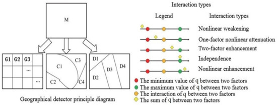
Figure 2.
Diagram of the geographical detector principles and interaction types [32,40] M: the study area; G1, G2, G3: the dependent variables used for detection (average WEPS from 2000 to 2015 as Y factor); C1, C2, C3, C4: sub-areas of impact factor C; D1, D2, D3, D4: sub-areas of impact factor D; q: explanatory power of the impact factors on the WEPS.
Changes in the WEPS are simultaneously affected by natural factors such as climate, soil, and vegetation types, as well as by human activities such as grazing withdrawal and grazing prohibition (see previous research [39,40]). In this study, eight natural factors and two socioeconomic factors were selected as detection factors and used to analyze the factors driving change in the average annual WEPS in the QTP from 2000 to 2015 (Table 1). Based on data types and operability, the landform types and soil types of the QTP were divided into 7 and 14 categories, respectively. The numerical variables were classified by the natural discontinuity method in ArcGIS. For example, the population density and GDP per unit area were divided into 5 categories, and the remaining variables were divided into 10 categories (Table 1).
2.2.5. Data Source
Meteorological datasets, including data on the daily temperature, precipitation, wind speed, and solar radiation data from 2000 to 2015, were acquired from meteorological stations. Snow cover data with a 25-km resolution were obtained from a long-term snow depth dataset [45], which was accessed from the Cold and Arid Region Science Data Center (http://westdc.westgis.ac.cn, accessed on 15 January 2022). NDVI values (spatial resolution 500 m) were derived from the international scientific data mirror website of the computer network information center of the Chinese Academy of Sciences (http://www.gscloud.cn, accessed on 15 January 2022). The DEM data (spatial resolution 30 m), GDP data (spatial resolution 1 km), 1:1,000,000 landform data, and land cover data (spatial resolution 1 km) were derived from the Resource and Environment Data Cloud Platform of the Chinese Academy of Sciences (CAS) (http://www.resdc.cn, accessed on 15 January 2022). The 1:1,000,000 soil data shapefile was provided by the Harmonized World Soil Database (HWSD) developed by the International Institute for Applied System Analysis (IIASA) of FAO. During the calculation, the international soil texture classification criteria in the database were converted to American criteria to meet the factor calculation requirements by using the logistic growth model proposed by Skaggs [42]. The 1:4 million calcium carbonate content data were accessed from the Data Sharing Infrastructure of Earth System Science (http://www.geodata.cn, accessed on 15 January 2022). All of the above data were resampled to a 1 km spatial resolution.
3. Results
3.1. WEPS and Its Monetary Value in the QTP
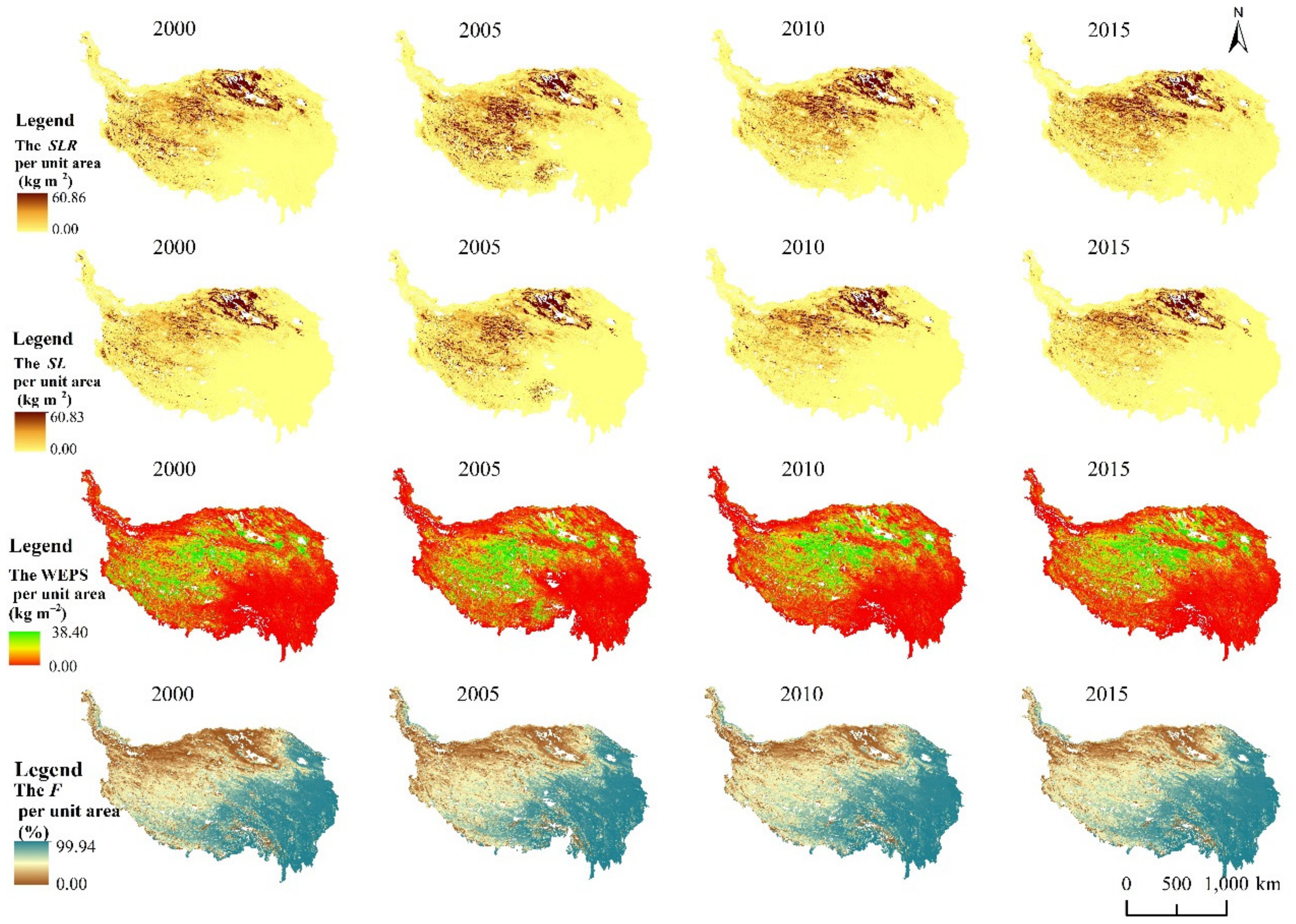
From 2000 to 2015, the total SLR (potential wind erosion) in the QTP was computed to range from 56.36 × 10⁸ t to 68.13 × 10⁸ t. There was an increase of 5.67 × 10⁸ t, and a trend of “rising–declining–declining” was shown. The SLR per unit area was calculated to be from 0 to 60.86 kg m−2, and the average SLR per unit area was estimated to be from 2.40 kg m−2 to 2.95 kg m−2 (Figure 2). The SLR per unit area was higher in the western and northern parts, whereas it was lower in the southeastern parts. This shows that the western and northern areas of the QTP, which contain desert areas, are more threatened by wind erosion.
The total SL (actual wind erosion) in the QTP was calculated to be from 38.55 × 10⁸ t to 43.39 × 10⁸ t during the year (Figure 3). Compared to 2000, the total SL was 0.65 × 10⁸ t lower in 2015. The SL per unit area was the highest in 2005, reaching 60.83 kg m−2, and a continuous decline occurred from 2005 to 2015. The average SL per unit area was estimated to be 1.67 kg m−2, 1.90 kg m−2, 1.75 kg m−2, and 1.65 kg m−2 in 2000, 2005, 2010, and 2015, decreasing by 0.02 kg m−2. The SL per unit area was higher in the northern and western parts and lower in the eastern and southern parts. This shows that strong wind erosion occurred in the northern and western areas of the QTP. In addition, when comparing the SL and SLR in the western area, it can be seen that the vegetation cover significantly reduced the occurrence of wind erosion (Figure 1 and Figure 3).

Figure 3.
The amount of WEPS, SLR, SL, and F per unit area of the QTP from 2000 to 2015.
The total WEPS in the QTP was computed as 17.48 × 10⁸ t in 2000 and 25.15 × 10⁸ t in 2015, and the total monetary value was estimated to be 22.36 × 10⁸ CNY in 2000 and 30.52 × 10⁸ CNY in 2015. The WEPS decreased by 6.39 × 10⁸ t in 2015 compared with the value in 2000, and its monetary value was reduced by 8.17 × 10⁸ CNY. The WEPS per unit area was calculated to range from 0 to 38.40 kg m−2 in 2000 to 2015 (Figure 2), and the average WEPS per unit area was estimated to be from 0.09 kg m−2 to 0.13 kg m−2. The WEPS per unit area was higher in the central and southwestern parts of the QTP, where grassland is the main land type, whereas it was found to be lower in the northern parts (Figure 1 and Figure 3). It can be speculated that the grassland distribution area played a major role in preventing wind erosion in the QTP.
The average F value (retention rate of WEPS) in the QTP was between 57.24% and 62.10% from 2000 to 2015 (similar to that found in previous research [10]), showing an increasing trend. The F value was calculated to range from 0 to 99.94%. Different from the inter-annual variation in the WEPS, potential wind erosion, and actual wind erosion values, the retention rate of the WEPS in the QTP was highest in 2015 and lowest in 2000. Areas with higher WEPS retention rate were mainly located in the southeast where there is better vegetation coverage (Figure 1). A relatively obvious geographical distribution from northwest to southeast was shown.
3.2. WEPS and Its Monetary Value of Different Province and Cities in the QTP
Among the provinces in the QTP, Qinghai and the Tibet Autonomous Region were found to account for more than 90% of the WEPS. The total WEPS in Tibet showed the highest value, reaching 16.15 × 10⁸ t in 2005, and its monetary value was calculated as 20.66 × 10⁸ CNY. This was followed by Qinghai Province and Yunnan Province.
From 2000 to 2015, there were significant differences in the WEPS. The total WEPS in Xinjiang showed a gradual increasing trend over time, and the other four provinces showed a trend of “rising–declining”. The Tibet Autonomous Region and Yunnan Province reached the highest total WEPS values in 2005, whereas in 2010, the maximum values occurred in Qinghai and Sichuan (Figure 4). The total WEPS in all provinces increased from 2000 to 2015, with Qinghai Province showing the largest increase of 3.55 × 10⁸ t, followed by the Tibet Autonomous Region. It can be concluded that Tibet and Qinghai have greater WEPS concentrations.
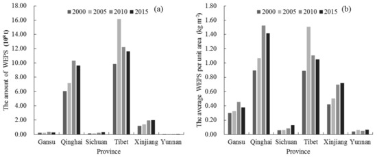

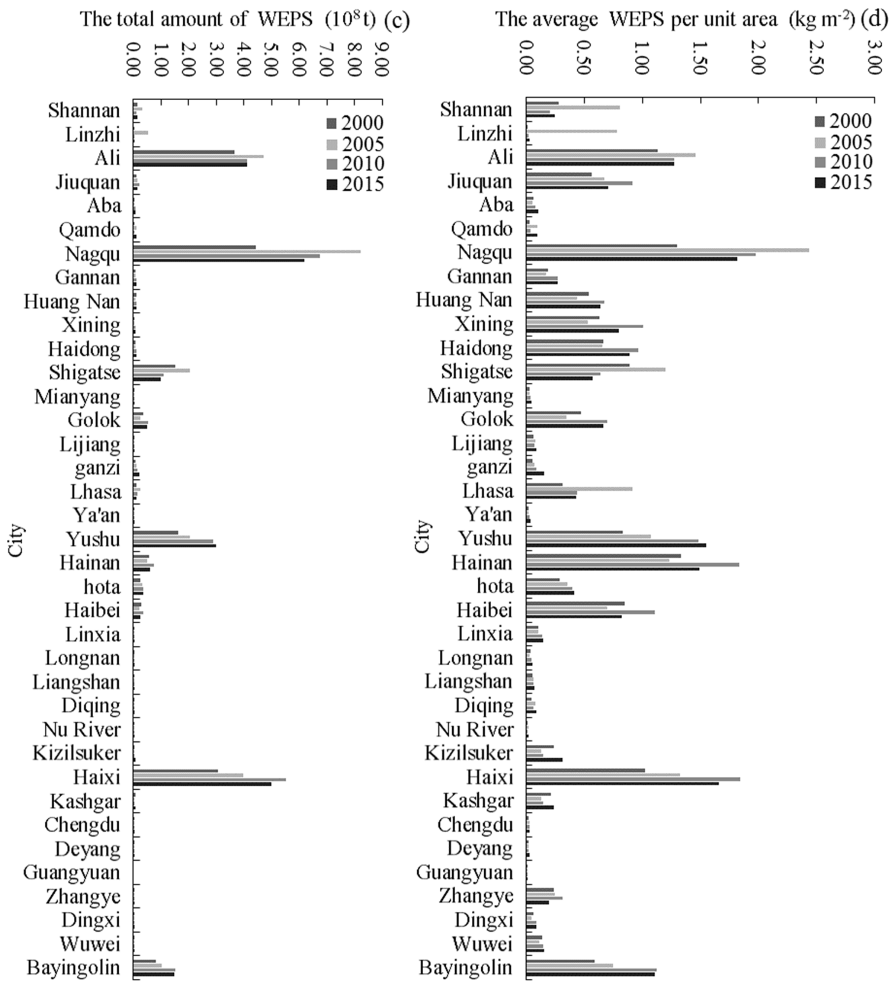
Figure 4.
The WEPS in different provinces (a,b) and cities (c,d) in the QTP from 2000 to 2015.
In 2000, 2010, and 2015, the average WEPS per unit area was the highest for Qinghai province with values of 0.89 kg m−2, 1.52 kg m−2, and 1.42 kg m−2, whereas in 2005, the Tibet Autonomous Region had the highest average WEPS per unit area, and the Yunnan province had the lowest values. From 2000 to 2015, the average WEPS per unit area in Sichuan province showed a gradual increasing trend over time, and that in Yunnan showed a trend of “rising-declining-rising”. The other three provinces showed a trend of “rising-declining”. However, the average WEPS per unit area increased for all provinces, with that in Qinghai increasing the most at 0.52 kg m−2, followed by Xinjiang with 0.30 kg m−2.
Among the 37 cities in the QTP, Nagqu was shown to have the highest total WEPS, accounting for 25–33% of the total. In 2015, its total WEPS amounted to 6.17 × 10⁸ t. This was followed by Haixi, accounting for 16–22%. From 2010 to 2015, all cities showed a trend of “rising–declining”. Compared with 2000, the total WEPS decreased in Shannan, Shigatse, Haibei, and Zhangye in 2015. Shigatse decreased by 0.54 × 10⁸ t. Zhangye decreased the least, by only 0.06 × 10⁸ t. The largest increase in the WEPS occurred in Haixi, where there was an increase of 1.91 × 10⁸ t, followed by Naqu and Yushu, which increased by 0.19 × 10⁸ t and 0.17 × 10⁸ t, respectively.
In 2000, the average WEPS per unit area was the highest for Hainan Region at 1.33 kg m−2, whereas during 2005 and 2015, Naqu reached the highest average WEPS per unit area with a range from 1.82 to 2.43 Guangyuan city had the lowest WEPS per unit area. From 2000 to 2015, the average WEPS per unit area in cities such as Mianyang, Ganzi, Ya’an, Yushu, Chengdu, Deyang, and Guangyuan showed a gradual increasing trend over time. In Shannan, Shigatse, Haibei, and Zhangye there was a volatile decreasing trend, whereas in other cities, a volatile growing trend was shown. Compared with 2000, the average WEPS per unit area in Yushu increased the most (0.71 kg m−2), followed by Haixi with 0.64 kg m−2. The average WEPS per unit area decreased the most in Shigatse (by 0.32 kg m−2). Overall, the WEPS in most of the cities in the QTP improved.
3.3. WEPS and Its Monetary Value of Different Ecosystems in the QTP
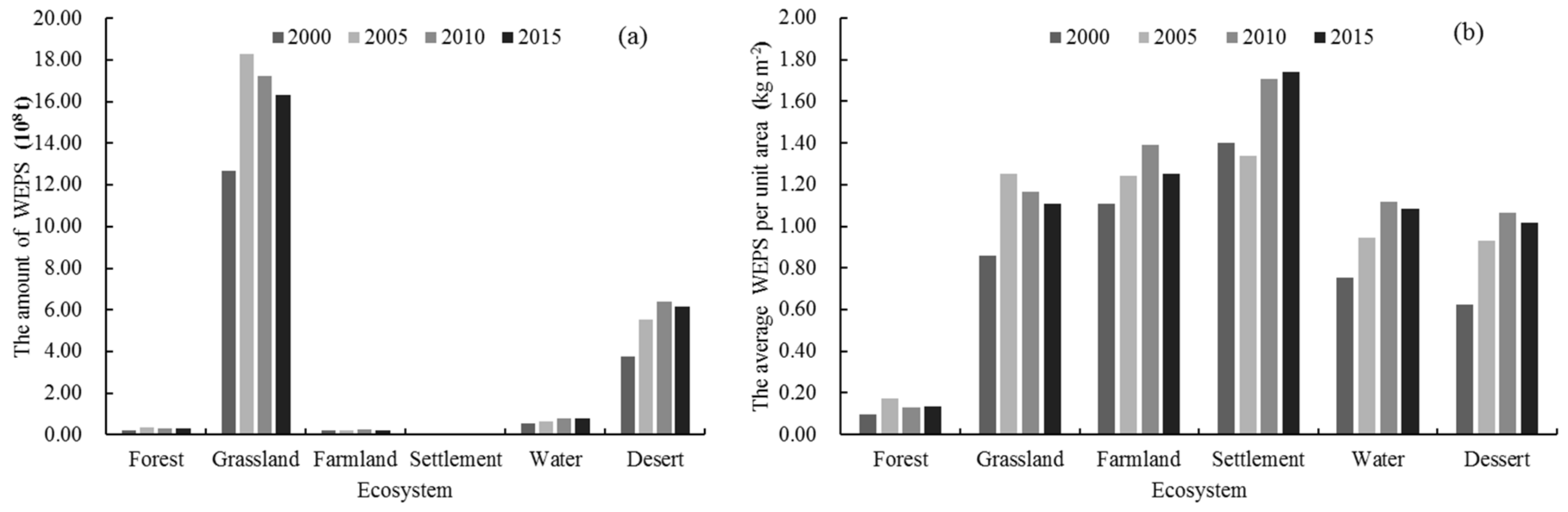
Among the different types of ecosystems in the QTP, the grassland ecosystem has the highest WEPS, accounting for more than 68% of the total. The WEPS of the grassland ecosystem was estimated to range from 12.7 × 10⁸ t to 18.29 × 10⁸ t from 2010 to 2015. The monetary value was calculated to be from 16.24 × 10⁸ CNY to 23.39 × 10⁸ CNY. The settlement ecosystem had the lowest WEPS. In 2015, the average WEPS per unit area was the highest for the grassland ecosystem, 8.06 kg m−2, followed by the settlement ecosystem, and the value for the forest ecosystem was the lowest. From 2000 to 2015, the total WPES in all ecosystems showed an increasing trend, among which the forest ecosystem increased the most, reaching 3.61 × 10⁸ t, followed by the desert ecosystem (Figure 5).
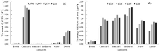
Figure 5.
The total (a) and average (b) WEPS of different ecosystems in the QTP from 2000 to 2015.
3.4. Change of Spatial Pattern of WEPS in the QTP
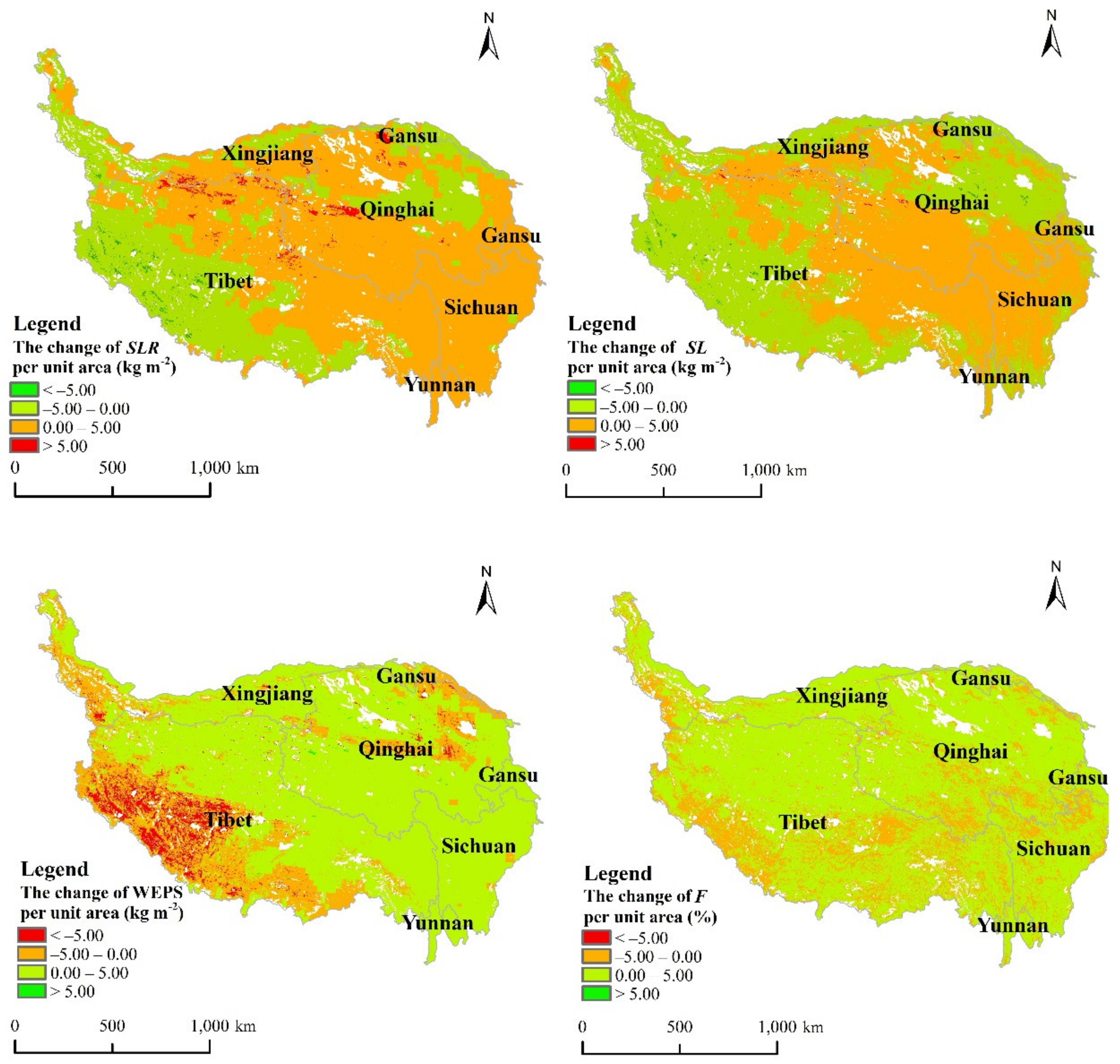
From 2000 to 2015, the change in SLR per unit area in the QTP ranged from −27.74 kg m−2 to 15.29 kg m−2, with an average change of 0.24 kg m−2. An increase in SLR per unit area mainly occurred in the western areas of northeastern QTP, on the eastern edge, and in the central and northern parts of the area. Both the central and western parts showed a downward trend, especially the western part. The change in SL per unit area in the QTP ranged from −27.04 kg m−2 to 13.03 kg m−2, with an average change of 0.02 kg m−2. An increase in SL per unit area mainly occurred in northeastern QTP, on the eastern edge, and in the central and northern parts. Both the central and western parts showed a downward trend.
The change in WEPS per unit area in the QTP ranged from −14.85 kg m−2 to 20.40 kg m−2, with an average change of 0.26 kg m−2. Increases in the WEPS per unit area mainly occurred in the western part of northeastern QTP, on the eastern edge, and in the central and northern parts. Both the central and western parts showed a downward trend. The WEPS per unit area increased most significantly in Huzuoqi, Xinbalhuyouqi, and Chenbalhu in the west of Hulunbuir. In Zhenglan Banner in the southeast of Xilin Gol League, West Uzhumuqin in the northwest, the central and northern parts of Chifeng City, and the southeast of Ulanchabu City, the decline in the WEPS per unit area was more significant. From 2000 to 2015, the change in F per unit area in the QTP ranged from −89.17% to 97.89%, with an average change of 5.00%. A decrease in F per unit area mainly occurred in the western parts of northeastern QTP, on the eastern edge, and in the central and northern parts. Both the central and western parts showed an upward trend (Figure 6).

Figure 6.
The changes in the WEPS, SLR, SL, and F per unit area in the QTP from 2000 to 2015.
3.5. WEPS in the QTP and the Detection of Its Driving Forces
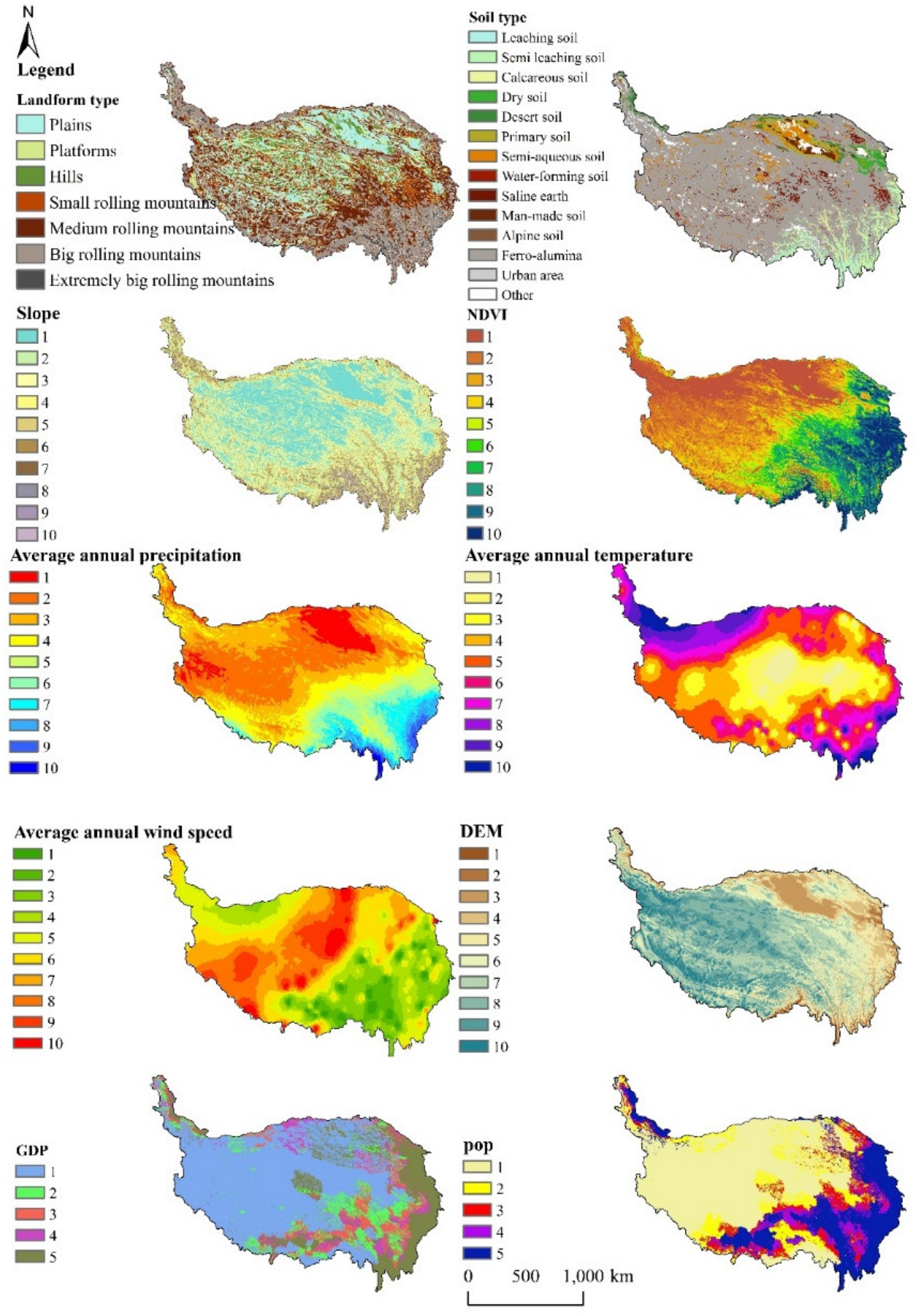
This study set the grade of the average annual WEPS per unit area from 2000 to 2015 as the Y factor, and 23,853 samples were generated using geographic detectors to match and extract attribute values with other raster data layers (Figure 7). The landform type, soil type, slope, average annual NDVI, average annual precipitation, average annual temperature, average annual wind speed, DEM, average annual gross domestic product (GDP), and average annual population density were set as factors X1–X10 (Figure 8). The results show that the detected q values were as follows: slope (0.440) > landform type (0.275) > average annual precipitation (0.223) > average annual wind speed (0.186) > average annual NDVI (0.142) > average annual population density (0.124) > average annual GDP (0.076) > DEM (0.071) > average annual temperature (0.057) > soil type (0.053) (Table 2). Slope was found to be the most important factor controlling the spatial differentiation of the WEPS, followed by landform type, average annual precipitation, and average annual wind speed. The WEPS grade was not significantly affected by the average annual temperature or soil type. The influences of human factors, such as the average annual population density and average annual GDP, on the grade of the average annual WEPS tended to be less than the influences of most natural factors, which indicates that natural factors have dominated the formation of wind erosion in the area, but human activities have still had an impact on the WEPS in the QTP.
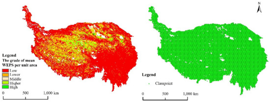
Figure 7.
The grade of the average annual WEPS per unit from 2000 to 2015 and samples.

Figure 8.
WEPS factors detected in the QTP.
Table 2.
Result of factor detection.
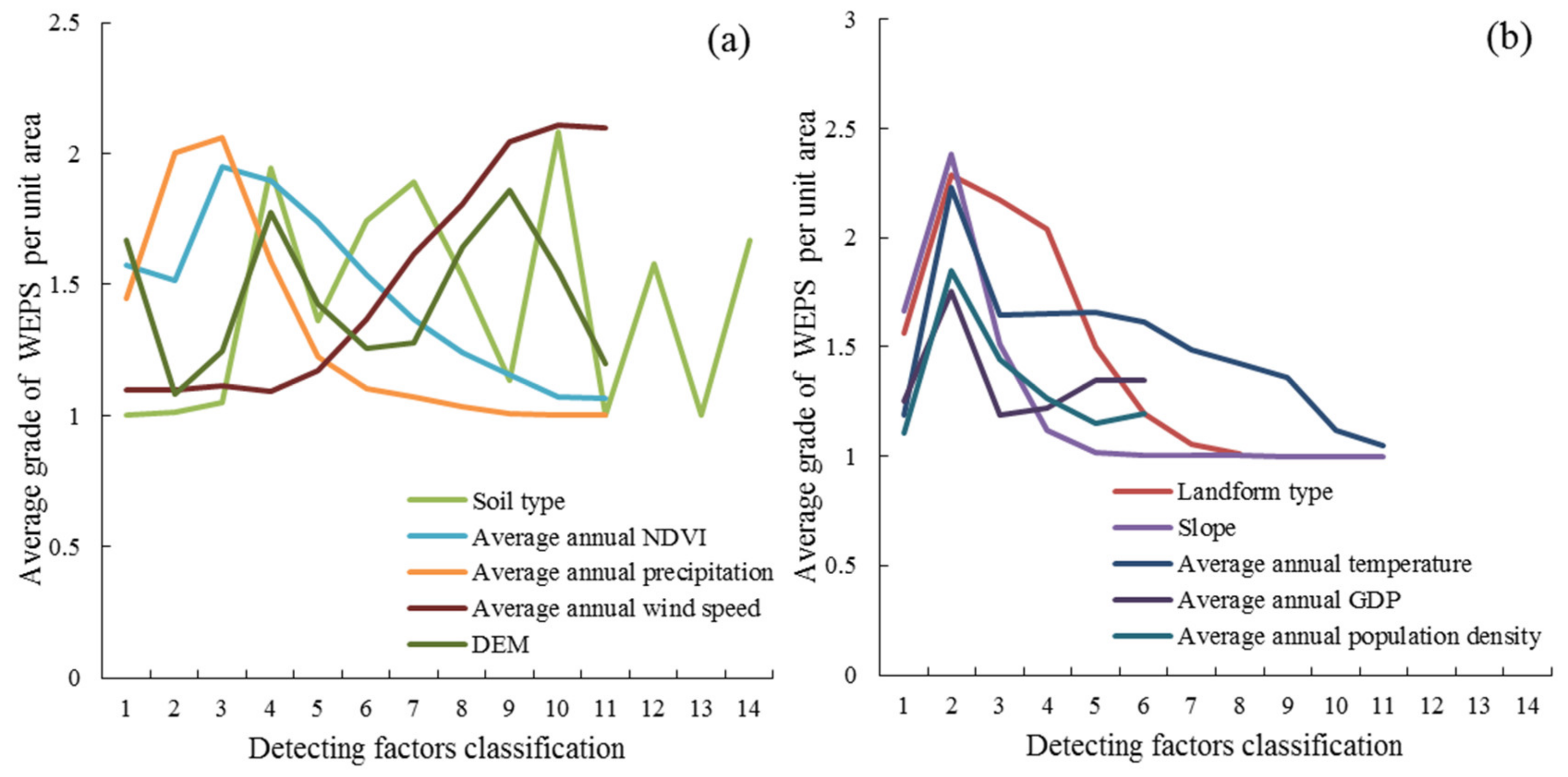
The risk detector was used to detect the areas with the highest WEPS grade for each factor partition to reveal the internal mechanism responsible for the spatial pattern of the WEPS. The risk detection results show that, as the average annual wind increased, the average WEPS grade per unit area gradually increased. As the slope, average annual precipitation, average annual precipitation temperature, average annual GDP, and average annual population density increased, the average WEPS grade per unit area showed a trend of increasing and then decreasing. The highest WEPS grade occurred when the DEM ranged from 5074 m to 5458 m (Table 1, Figure 9). The average annual GDP and average annual population density trends show that appropriate levels of human activity can help to improve the WEPS grade, but excessive human disturbance in areas with moderate economic development and population density can lead to lower WEPS levels. However, the WEPS grade in the most economically developed areas was higher than that in the moderately developed areas, which could be due to the greater investment in, and influence of, environmental protection measures.
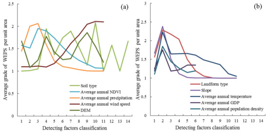
Figure 9.
Average WEPS grade per unit area in relation to the classification of different detected factors. Note: (a) present the average WEPS grade per unit area in the classification of soil type, average annual NDVI, average annual precipitation, average annual wind speed, and DEM; (b) present the average WEPS grade per unit area in the classification of landform type, slope, average annual temperature, average annual GDP, and average annual population density.
The results for the detected factors (Table 3) show that the average annual precipitation, average annual GDP, and average annual population density were significantly different from all the other influencing factors. Landform type, slope, average annual NDVI, average annual wind speed, and average annual temperature showed significant differences with most of the other influencing factors, whereas the DEM showed no significant differences with most of the influencing factors.
Table 3.
Statistical significance between detecting factors.
The multi-year average interaction detector results (Table 4) showed that each factor had an enhanced interaction effect on the WEPS of the QTP. Landform type, soil type, average annual NDVI, and average annual precipitation showed nonlinear enhancement relationships with other factors. Slope, average annual temperature, average annual wind speed, DEM, average annual GDP, and average annual population density showed nonlinear enhancement relationships with other factors. The two-factor enhancement between the slope and other factors was found to have a greater impact on the spatial variation of the WEPS grade, and the degree of influence (q value) on the WEPS grade exceeded 44%, which showed that the slope also strengthened the influences of other factors on the spatial distribution of the WEPS.
Table 4.
Interaction type and q value between different detecting factors.
However, the nonlinear enhancement relationship between the annual average temperature and other factors was found to have a high degree of influence on the spatial variation of the WEPS with a nonlinear enhancement for all factors. It can be concluded that although the single-factor effect of the annual mean temperature and the soil type on the spatial variation of the WEPS were weak, the interaction between the two factors had a higher level of influence on the WEPS than the two factors alone by changing the regional natural environment or human activities. This suggests that the sum of the individual effects of two factors indirectly affects the spatial variation of the WEPS.
4. Discussion
The change pattern of the WEPS was similar to that of the SLR (Figure 6), mainly because the WEPS is more dependent on natural factors, such as the slope, precipitation, and wind. As shown in previous studies, soil type played an important role in the spatial distribution pattern of the sand-stabilization service function [40], soil wind erosion rate was intensified significantly with increasing wind velocities by a power function [46], and the increase in rainfall reduced wind erosion [10]. It seems to be proven that climate changes are the leading factors that affect the soil wind erosion in a region overall, which is consistent with the finding of Li et al. [47].
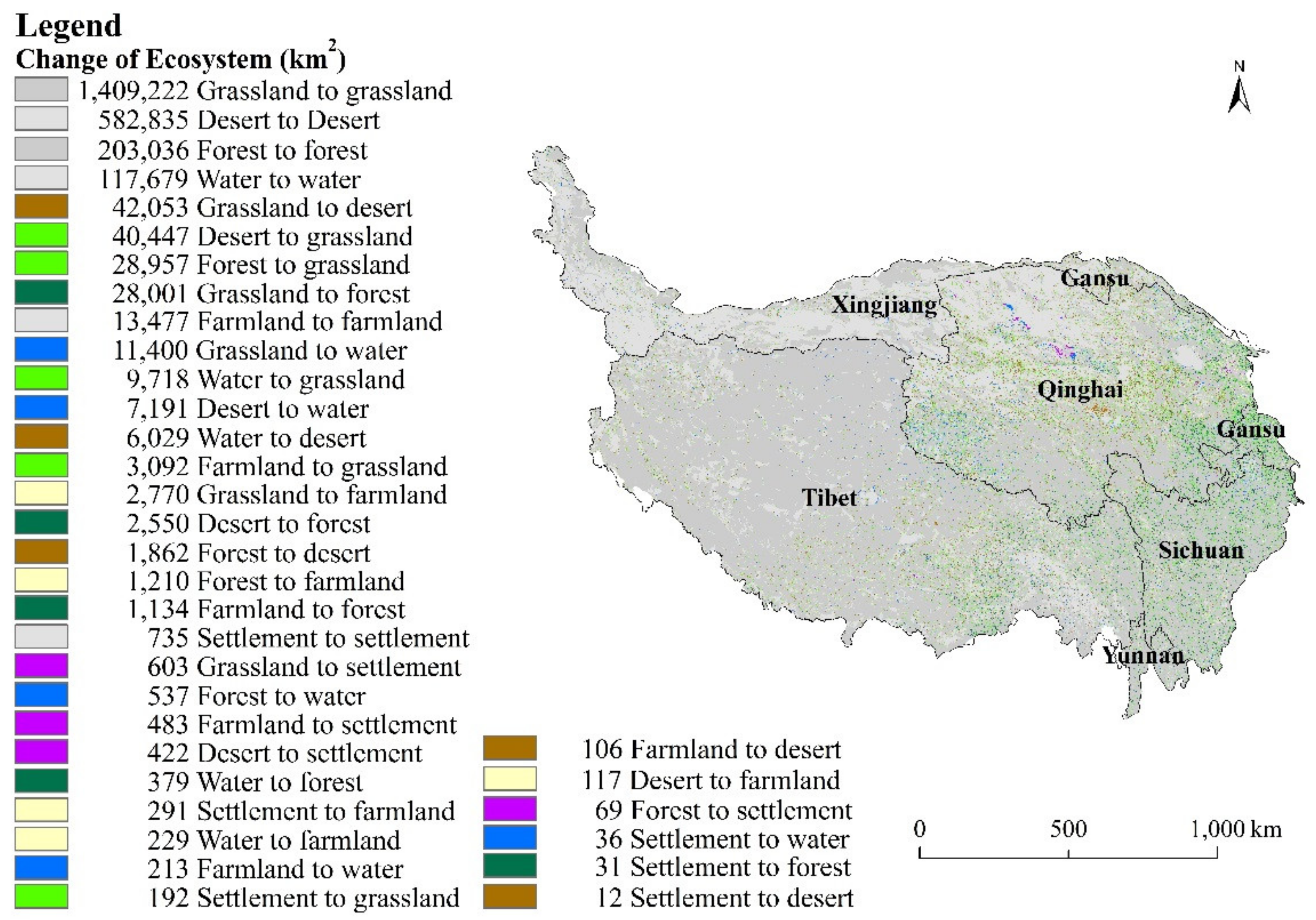
Increasing fractional vegetation cover can effectively reduce the amount of soil erosion. People can change factors such as the NDVI by improving vegetation coverage and reducing the SL. From 2000 to 2015, a series of ecological conservation and restoration programmes and policies such as Grazing Forbidden Policy and the Grassland Ecological Protection Subsidies and Rewards Program have been implemented in the QTP, which have proven to be effective in reducing soil wind erosion [10]. In terms of changes in land use from 2000 to 2015, the amount of area translated from grassland ecosystem to desert ecosystem was the highest, followed by that from desert to grassland. The increase in the forest ecosystem area was mainly due to conversion from grassland and settlement areas (Figure 10). The change area mainly occurred in eastern part and southern edge of the QTP, where human activities are concentrated [48,49].

Figure 10.
The area changes in ecosystems in the QTP from 2000 to 2015 (km2).
Among the different types of land use change, the increase in the forest ecosystem area caused an increase in the WEPS, whereas the increase in the desert ecosystem area caused a decrease in the average WEPS in the QTP. The average WEPS per unit area only decreased in the area that was transformed from a water ecosystem to a settlement ecosystem (Figure 11). As same as the result shown in Chi’s study [4], the land use/cover change (such as returning farmland to forest, shrub, and grassland) played a key role in reducing the soil wind erosion modulus and enhancing regional WEPS. It was found that the increase in grassland area played a certain role in improving the WEPS due to the control of desertification and the implementation of the returning farmland to grassland project. However, due to unsuitable land use, the resulting significant increase in the desert area is the main reason for the decrease in the total WEPS.
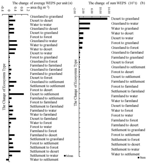
Figure 11.
The change of mean and sum WEPS in different ecosystem in the QTP from 2000 to 2015.
Because land use change played an important role in WEPS change in QTP, reasonable land use management will help to promote regional ecological environment protection and sustainable development. In this study, grassland and desert changed significantly, over-grazing, logging, and crop planting have resulted in significant vegetation degradation and desertification, but the implementation of ecological protection projects has promoted the area of grassland and forest [50,51]. For further management, the grassland and desert in the eastern and south-eastern parts of the QTP could be restored to forests engineering practices, plantations, enclosures to limit human disturbances, etc., and the most widely adopted practice in the north and western part of the QTP should be natural restoration. In addition, water shortages in arid and semiarid regions were neglected and the conservation of water bodies should receive more attention.
5. Conclusions
This current study assessed spatial–temporal changes of the WEPS in the QTP from 2000 to 2015. The spatial dynamics of the WEPS were analyzed from the perspectives of various leagues and cities and ecosystems, and its driving forces such as contributions of influential factors to the WEPS and their interactions using geo-detector. The results indicate the following conclusions.
Areas with moderate and high soil erosion intensities were mainly distributed in the western and northern QTP, which contain distributed massive desert and sparse grassland. The annual mean WEPS showed an increasing trend from 2000 to 2015. Slope and weather factors, such as precipitation and wind speed, played leading roles in determining the spatial pattern and grade of the WEPS, and human activities showed an important factor in the variation of WEPS.
In addition, the implementation of projects, such as returning farmland to grassland and desertification control, increased the WEPS by increasing the grassland area. The increase in the desert ecosystem area due to unsuitable land use resulted in a significant reduction in the WEPS in the QTP.
However, there were still some limitations in our study. First, due to the lack of field observation data, this study did not consider the seasonal variation in the wind velocity threshold, thus the seasonal difference in the WEPS could not be analyzed. Second, further parameter localization in the determination of the erodibility boundary of the RWEQ model should be executed in the future to improve the accuracy of the simulation results. Finally, the study of the factors driving the WEPS using the geographic detector model showed the relationships among different factors, whereas the coupling effects of natural factors and human factors need to be studied further.
Author Contributions
Conceptualization, G.X. and Y.X.; methodology, J.X.; software, M.H.; validation, Y.W.; formal analysis, Y.W.; investigation, Y.W.; resources, S.G. and Y.N.; data curation, Y.W.; writing—original draft preparation, Y.W.; writing—review and editing, Y.X. and K.Q.; visualization, Y.X.; supervision, G.X., J.L. and L.Z.; project administration, Y.X.; funding acquisition, G.X. All authors have read and agreed to the published version of the manuscript.
Funding
This work was funded by the Strategic Priority Research Program of Chinese Academy of Sciences (XDA20020402), the National Natural Science Foundation of China (41971272), the Guangxi Science and Technology Major Project (AA20161002-3) and the Zhejiang Provincial Natural Science Foundation of China under Grant (LY18D010001).
Data Availability Statement
All data in this study were correctly referenced. Meteorological datasets, including data on the daily temperature, precipitation, wind speed, and solar radiation data from 2000 to 2015, were acquired from meteorological stations. Snow cover data with a 25-km resolution were obtained from a long-term snow depth dataset [45], which was accessed from the Cold and Arid Region Science Data Center (http://westdc.westgis.ac.cn, accessed on 15 January 2022). NDVI values (spatial resolution 500 m) were derived from the international scientific data mirror website of the computer network information center of the Chinese Academy of Sciences (http://www.gscloud.cn, accessed on 15 January 2022). The DEM data (spatial resolution 30 m), GDP data (spatial resolution 1 km), 1:1,000,000 landform data, and land cover data (spatial resolution 1 km) were derived from the Resource and Environment Data Cloud Platform of the Chinese Academy of Sciences (CAS) (http://www.resdc.cn, accessed on 15 January 2022). Achievement of the geographic detector was operated with geo-detector software [44] (http://geo-detector.cn/, accessed on 15 January 2022).
Conflicts of Interest
The authors declare no conflict of interest.
References
- Xie, G.D.; Lu, C.X.; Leng, Y.F.; Zheng, D.; Li, S.C. Ecological assets valuation of the Tibetan Plateau. J. Nat. Resour. 2003, 18, 189–196. (In Chinese) [Google Scholar]
- Li, X.W.; Li, M.D.; Dong, S.K.; Shi, J.B. Temporal-spatial changes in ecosystem services and implications for the conservation of alpine rangelands on the Qinghai-Tibetan Plateau. Rangel. J. 2015, 37, 31–43. [Google Scholar] [CrossRef]
- Yang, C.; Geng, Y.; Fu, X.Z.; Coulter, J.A.; Chai, Q. The effects of wind erosion depending on cropping system and tillage method in a semi-arid region. Agronomy 2020, 10, 732. [Google Scholar] [CrossRef]
- Chi, W.; Zhao, Y.; Kuang, W.; He, H. Impacts of anthropogenic land use/cover changes on soil wind erosion in China. Sci. Total Environ. 2019, 668, 204–215. [Google Scholar] [CrossRef] [PubMed]
- Meng, N.; Yang, Y.-Z.; Zheng, H.; Li, R.-N. Climate change indirectly enhances sandstorm prevention services by altering ecosystem patterns on the Qinghai-Tibet Plateau. J. Mt. Sci. 2021, 18, 1711–1724. [Google Scholar] [CrossRef]
- Wang, X.; Lang, L.; Yan, P.; Wang, G.; Li, H.; Ma, W.; Hua, T. Aeolian processes and their effect on sandy desertification of the Qinghai-Tibet Plateau: A wind tunnel experiment. Soil Tillage Res. 2016, 158, 67–75. [Google Scholar] [CrossRef]
- Huang, K.; Zhang, Y.; Zhu, J.; Liu, Y.; Zu, J.; Zhang, J. The influences of climate change and human activities on vegetation dynamics in the Qinghai-Tibet Plateau. Remote Sens. 2016, 8, 876. [Google Scholar] [CrossRef] [Green Version]
- Ping, Y.; Zhibao, D.; Guangrong, D.; Zhang, X.; Yiyun, Z. Preliminary results of using 137 Cs to study wind erosion in the Qinghai-Tibet Plateau. J. Arid Environ. 2001, 47, 443–452. [Google Scholar] [CrossRef]
- Li, Q.; Zhang, C.; Zhou, N.; Shen, Y.; Wu, Y.; Zou, X.; Li, J.; Jia, W.; Wang, X. Spatial distribution of Aeolian desertification on the Qinghai-Tibet Plateau. J. Desert Res. 2018, 38, 690–700. [Google Scholar] [CrossRef]
- Teng, Y.M.; Zhan, J.Y.; Liu, W.; Sun, Y.; Boappeah Agyemang, F.; Zhihui, L. Spatiotemporal dynamics and drivers of wind erosion on the Qinghai-Tibet Plateau, China. Ecol. Indicators 2021, 123, 107340. [Google Scholar] [CrossRef]
- Bagnold, R.A.; Sandford, K.S.; Shaw, W.B.K. A further journey through the Libyan Desert (continued). Geogr. J. 1933, 82, 211–235. [Google Scholar] [CrossRef]
- Woodruff, N.P.; Siddoway, F.H. A Wind Erosion Equation. Proc. Soil Sci. Soc. Am. 1965, 29, 602–608. [Google Scholar] [CrossRef]
- Gregory, J.M.; Wilson, G.R.; Singh, U.B.; Darwish, M. TEAM: Integrated, process-based wind-erosion model. Environ. Model. Soft. 2004, 19, 205–215. [Google Scholar] [CrossRef]
- Lindstrom Usda-Ars, M.J. A description of devices used in the study of wind erosion of soils. Soil Sci. 1985, 140, 313. [Google Scholar] [CrossRef]
- Fryrear, D.W.; Bilbro, J.D.; Saleh, A. RWEQ: Improved wind erosion technology. J. Soil Water Conserv. 2000, 55, 183–189. [Google Scholar]
- Hagen, L.J. Evaluation of the Wind Erosion Prediction System (WEPS) erosion submodel on cropland fields. Environ. Model. Soft. 2004, 19, 171–176. [Google Scholar] [CrossRef]
- Van Pelt, R.S.; Zobeck, T.M.; Potter, K.N.; Stout, J.E.; Popham, T.W. Validation of the wind erosion stochastic simulator (WESS) and the revised wind erosion equation (RWEQ) for single events. Environ. Model. Soft. 2004, 19, 191–198. [Google Scholar] [CrossRef]
- Jiang, L.; Xiao, Y.; Ouyang, Z.; Xu, W.; Zheng, H. Estimate of the wind erosion modules in Qinghai Province based on RWEQ model. Res. Soil Water Conserv. 2015, 22, 21–25. (In Chinese) [Google Scholar] [CrossRef]
- Huang, L.; Cao, W.; Wu, D.; Gong, G. The temporal and spatial variations of ecological services in the Tibet Plateau. J. Nat. Resour. 2016, 31, 543–555. [Google Scholar]
- Jiang, C.; Li, D.; Wang, D.; Zhang, L. Quantification and assessment of changes in ecosystem service in the Three-River Headwaters Region, China as a result of climate variability and land cover change. Ecol. Ind. 2016, 66, 199–211. (In Chinese) [Google Scholar] [CrossRef]
- Zhang, C.; Gong, J.; Zou, X.; Dong, G.; Li, X.; Dong, Z.; Qing, Z. Estimates of soil movement in a study area in Gonghe Basin, north-east of Qinghai-Tibet Plateau. J. Arid Environ. 2003, 53, 285–295. (In Chinese) [Google Scholar] [CrossRef]
- Zhang, H.B.; Peng, J.; Zhao, C.N.; Xu, Z.H.; Dong, J.Q.; Gao, Y. Wind speed in spring dominated the decrease in wind erosion across the Horqin Sandy Land in northern China. Ecol. Indic. 2021, 127, 107599. [Google Scholar] [CrossRef]
- Jiang, C.; Yang, Z.; Wang, X.; Dong, X.; Li, Z.; Li, C. Examining the reversal of soil erosion decline in the hotspots of sandstorms: A non-linear ecosystem dynamic perspective. J. Arid Environ. 2021, 186, 104421. [Google Scholar] [CrossRef]
- Jiang, C.; Liu, J.G.; Zhang, H.Y.; Zhang, Z.D.; Wang, D.W. China’s progress towards sustainable land degradation control: Insights from the northwest arid regions. Ecol. Eng. 2019, 127, 75–87. [Google Scholar] [CrossRef]
- Lyu, X.; Li, X.B.; Wang, H.; Gong, J.R.; Li, S.K.; Dou, H.S.; Dang, D.L. Soil wind erosion evaluation and sustainable management of typical steppe in Inner Mongolia, China. J. Environ. Manag. 2021, 277, 111488. [Google Scholar] [CrossRef] [PubMed]
- Aubault, H.; Webb, N.P.; Strong, C.L.; Mc Tainsh, G.H.; Leys, J.F.; Scanlan, J.C. Grazing impacts on the susceptibility of rangelands to wind erosion: The effects of stocking rate, stocking strategy and land condition. Aeolian Res. 2015, 17, 89–99. [Google Scholar] [CrossRef]
- Zhang, H.Y.; Fan, J.W.; Cao, W.; Harris, W.; Li, Y.Z.; Chi, W.F.; Wang, S.Z. Response of wind erosion dynamics to climate change and human activity in Inner Mongolia, China during 1990 to 2015. Sci. Total Environ. 2018, 639, 1038–1050. [Google Scholar] [CrossRef]
- Latocha, A.; Szymanowski, M.; Jeziorska, J.; Stec, M.; Roszczewska, M. Effects of land abandonment and climate change on soil erosion—An example from depopulated agricultural lands in the Sudetes Mts., SW Poland. CATENA 2016, 145, 128–141. [Google Scholar] [CrossRef]
- Garbrecht, J.D.; Nearing, M.A.; Steiner, J.L.; Zhang, X.J.; Nichols, M.H. Can conservation trump impacts of climate change on soil erosion? Anassessment from winter wheat cropland in the Southern Great Plains of the United States. Weather Clim. Extrem. 2015, 10, 32–39. [Google Scholar] [CrossRef] [Green Version]
- Li, D.J.; Xu, D.Y.; Wang, Z.Y.; You, X.G.; Zhang, X.Y.; Song, A.L. The dynamics of sand—Stabilization services in Inner Mongolia, China from 1981 to 2010 and its relationship with climate change and human activities. Ecol. Indicators 2018, 88, 351–360. [Google Scholar] [CrossRef]
- Sharratt, B.S.; Tatarko, J.; Abatzoglou, J.T.; Fox, F.A.; Huggins, D. Implications of climate change on wind erosion of agricultural lands in the Columbia plateau. Weather Clim. Extrem. 2015, 10, 20–31. [Google Scholar] [CrossRef] [Green Version]
- Wang, J.F.; Xu, C.D. Geo-detector: Principle and prospective. Acta Geogr. Sinica 2017, 72, 116–134. [Google Scholar]
- Polykretis, C.; Alexakis, D.D. Spatial stratified heterogeneity of fertility and its association with socio-economic determinants using Geographical Detector: The case study of Crete Island, Greece. Appl. Geogr. 2021, 127, 102384. [Google Scholar] [CrossRef]
- Huang, J.X.; Wang, J.F.; Bo, Y.C.; Xu, C.D.; Hu, M.G.; Huang, D.C. Identification of health risks of hand, foot and mouth disease in China using the geographical detector technique. Int. J. Environ. Res. Public Health 2014, 11, 3407–3423. [Google Scholar] [CrossRef]
- Shen, J.; Zhang, N.; Gexigeduren, H.B.; Liu, C.Y.; Li, Y.; Zhang, H.Y.; Chen, X.Y.; Lin, H. Construction of a GeogDetector-based model system toindicate the potential occurrence of grasshoppers in Inner Mongolia steppe habitats. Bull. Entomol. Res. 2015, 105, 335–346. [Google Scholar] [CrossRef] [Green Version]
- Ren, Y.; Deng, L.Y.; Zuo, S.D.; Song, X.D.; Liao, Y.L.; Xu, C.D.; Chen, Q.; Hua, L.Z.; Li, Z.W. Quantifying the influences of various ecological factors on land surface temperature of urban forests. Environ. Pollut. 2016, 216, 519–529. [Google Scholar] [CrossRef] [Green Version]
- Liang, P.; Yang, X.P. Landscape spatial patterns in the Maowusu (Mu Us) Sandy Land, northern China and their impact factors. CATENA 2016, 145, 321–333. [Google Scholar] [CrossRef]
- Tian, F.; Liu, L.Z.; Yang, J.H.; Wu, J.J. Vegetation greening in more than 94% of the Yellow River Basin (YRB) region in China during the 21st century caused jointly by warming and anthropogenic activities. Ecol. Indicators. 2021, 125, 107479. [Google Scholar] [CrossRef]
- Li, J.; Wang, J.; Zhang, J.; Liu, C.; He, S.; Liu, L. Growing-season vegetation coverage patterns and driving factors in the China-Myanmar Economic Corridor based on Google Earth Engine and geographic detector. Ecol. Indic. 2022, 136, 108620. [Google Scholar] [CrossRef]
- Zhang, Y.; Xu, D.Y.; Wang, Z.Y.; Zhang, X.Y. The interaction of driving factors for the change of windbreak and sand-fixing service function in Xilingol League between 2000 and 2015. Acta Ecol. Sinica 2021, 41, 603–614. [Google Scholar]
- Du, H.Q.; Dou, S.T.; Deng, X.H.; Xue, X.; Wang, T. Assessment of wind and water erosion risk in the watershed of the Qinghai-Qinghai-Tibet Plateau Reach of the Yellow River, China. Ecol. Indicators 2016, 67, 117–131. [Google Scholar] [CrossRef]
- Skaggs, T.H.; Arya, L.M.; Shouse, P.J.; Mohanty, B.P. Estimating particle-size distribution from limited soil texture data. Soil Sci. Soc. Am. J. 2001, 65, 1038–1044. [Google Scholar] [CrossRef]
- Lv, C.Q. Study on Soil Carbon Stock and Its Spatial Distribution, Influence Factors in Tibetan Plateau. Master’s Thesis, Nanjing University, Nanjing, China, 2006. [Google Scholar]
- Wang, J.F.; Li, X.H.; Christakos, G.; Liao, Y.-L.; Zhang, T.; Gu, X.; Zheng, X.Y. Geographical detectors-based health risk assessment and its application in the neural tube defects study of the Heshun region, China. Int. J. Geograph. Inform. Sci. 2010, 24, 107–127. [Google Scholar] [CrossRef]
- Che, T.; Li, X.; Jin, R.; Armstrong, R.; Zhang, T. Snow depth derived from passive microwave remote-sensing data in China. Ann. Glaciol. 2008, 49, 145–154. [Google Scholar] [CrossRef] [Green Version]
- Xie, S.B.; Qu, J.J.; Wang, T. Wind tunnel simulation of the effects of freeze-thaw cycles on soil erosion in the Qinghai-Tibet Plateau. Sci. Cold Arid Reg. 2016, 8, 187–195. [Google Scholar]
- Li, J.; Ma, X.; Zhang, C. Predicting the spatiotemporal variation in soil wind erosion across Central Asia in response to climate change in the 21st century. Sci. Total Environ. 2020, 709, 136060. [Google Scholar] [CrossRef]
- Sun, Y.; Liu, S.; Shi, F.; An, Y.; Li, M.; Liu, Y. Spatio-temporal variations and coupling of human activity intensity and ecosystem services based on the four-quadrant model on the Qinghai-Tibet Plateau. Sci. Total Environ. 2020, 743, 140721. [Google Scholar]
- Wang, C.; Zhan, J.; Xin, Z. Comparative analysis of urban ecological management models incorporating low-carbon transformation. Technol. Forecast. Soc. Chang. 2020, 159, 120190. [Google Scholar] [CrossRef]
- Li, Y.; Li, J.; Are, K.; Huang, Z.; Yu, H.; Zhang, Q. Livestock grazing significantly accelerates soil erosion more than climate change in Qinghai-Tibet Plateau: Evidenced from 137Cs and 210Pbex measurements. Agric. Ecosyst. Environ. 2019, 285, 106643. [Google Scholar] [CrossRef]
- Pan, T.; Zou, X.; Liu, Y.; Wu, S.; He, G. Contributions of climatic and non-climatic drivers to grassland variations on the Tibetan Plateau. Ecol. Eng. 2017, 108, 307–317. [Google Scholar] [CrossRef]


Publisher’s Note: MDPI stays neutral with regard to jurisdictional claims in published maps and institutional affiliations. |
© 2022 by the authors. Licensee MDPI, Basel, Switzerland. This article is an open access article distributed under the terms and conditions of the Creative Commons Attribution (CC BY) license (https://creativecommons.org/licenses/by/4.0/).