
An Estimation of the Anthropogenic Heat Emissions in Darwin City Using Urban Microclimate Simulations

 ,
,  ,
,  ,
,  ,
,  ,
, 
Abstract
:1. Introduction
2. Methodology
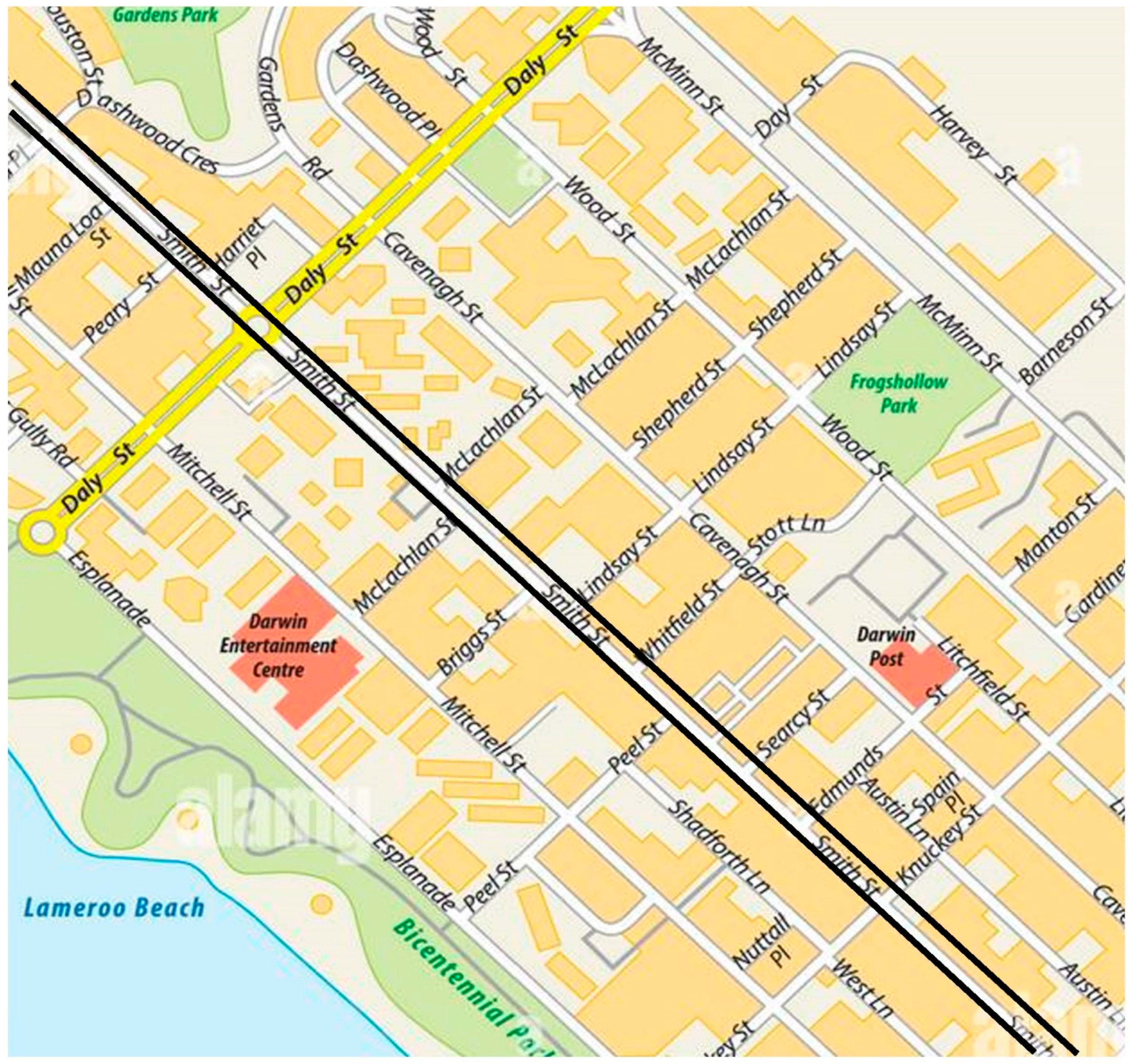
2.1. Area of Study
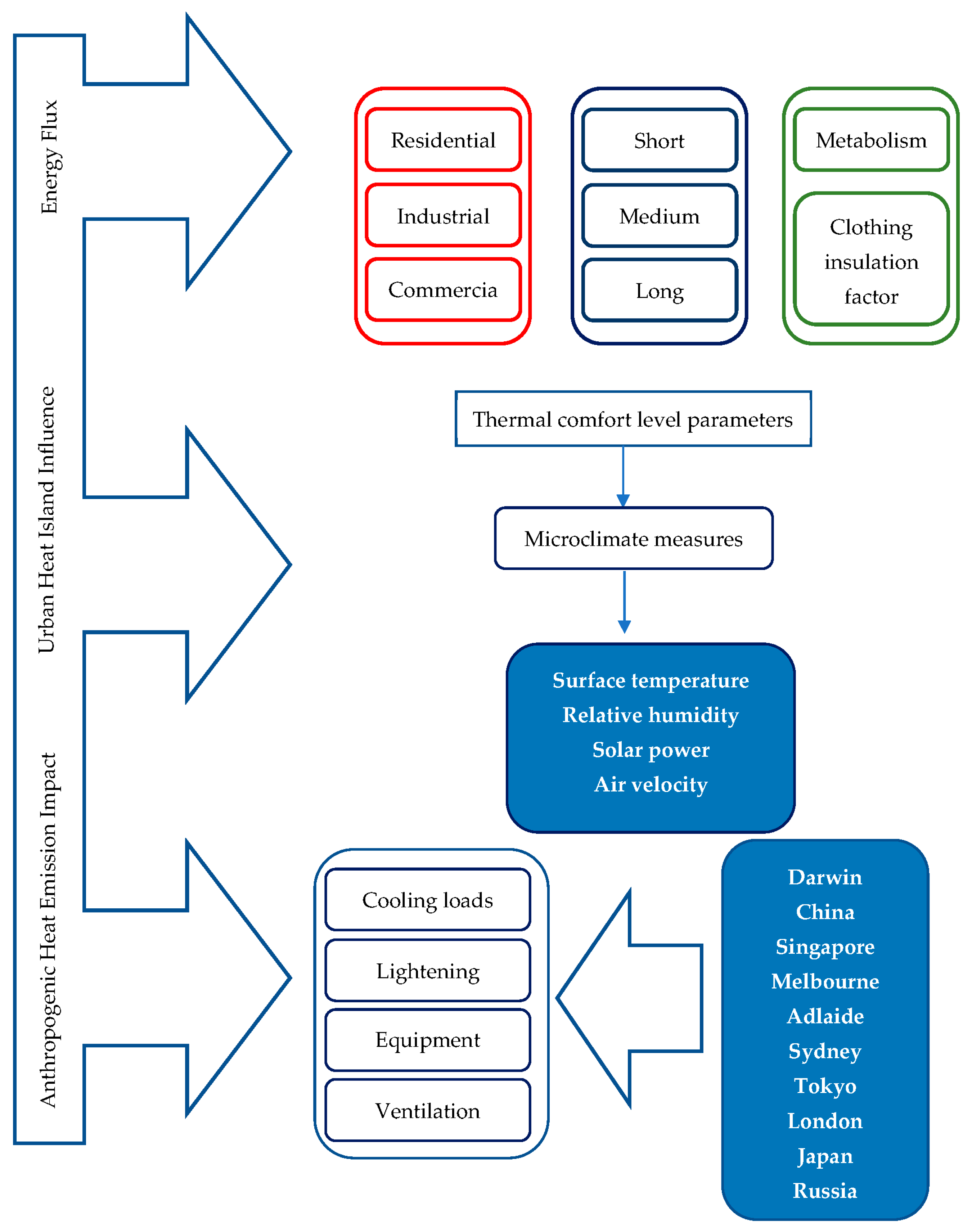
2.2. Adopted Study Approach
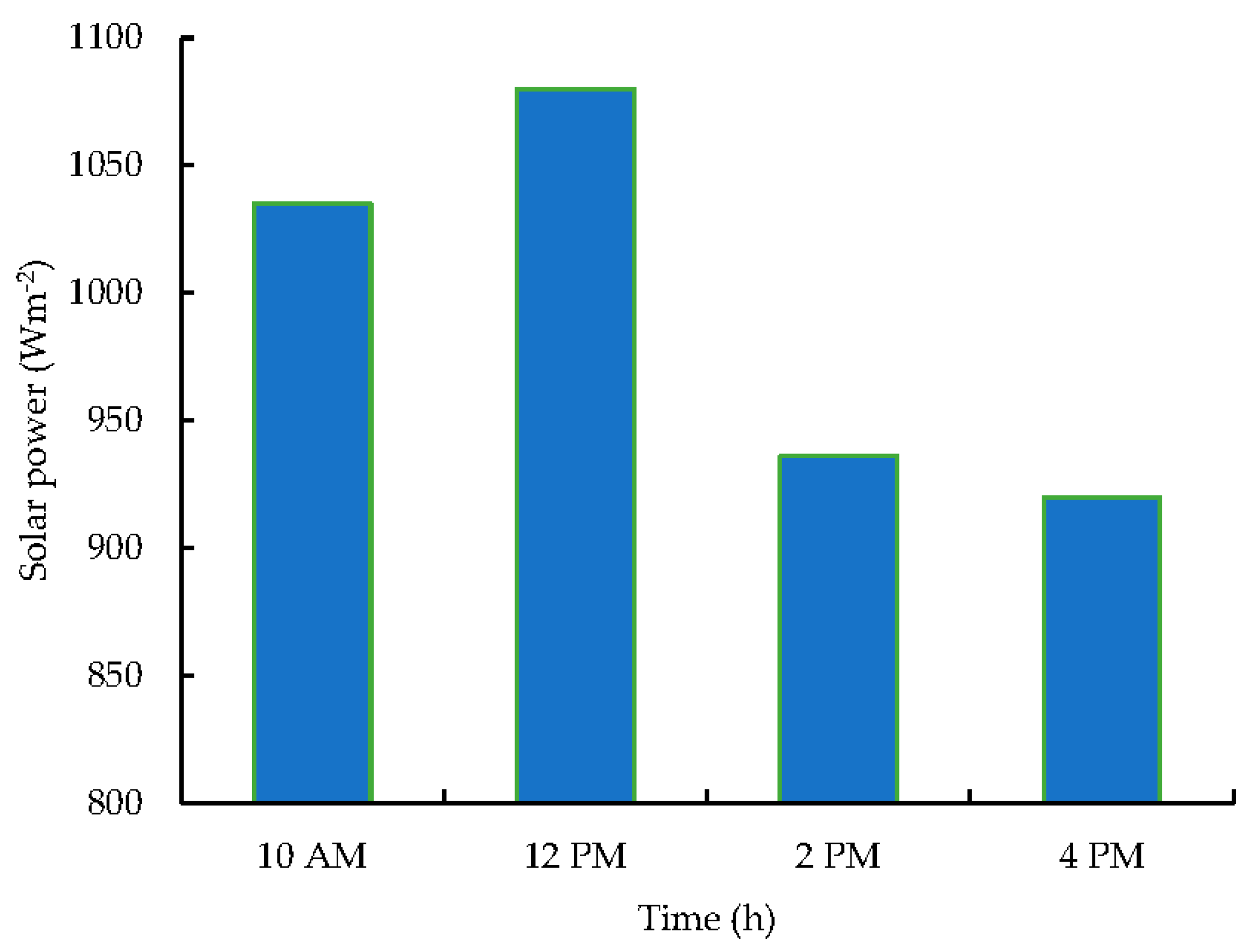
2.3. Microclimate (Temperature and Humidity Variation) Measurements
2.4. Estimation of Anthropogenic Heat Emission Factors
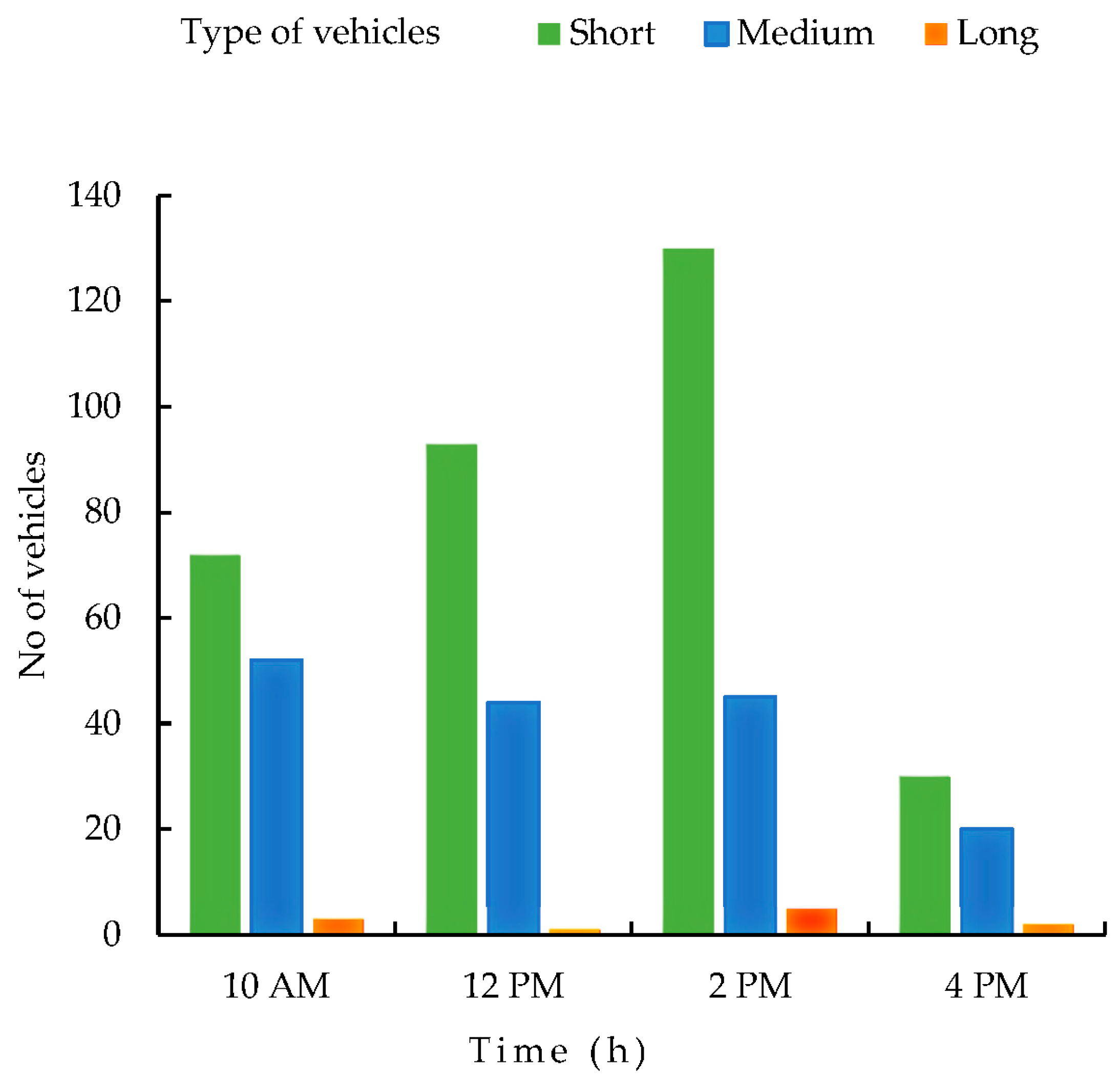
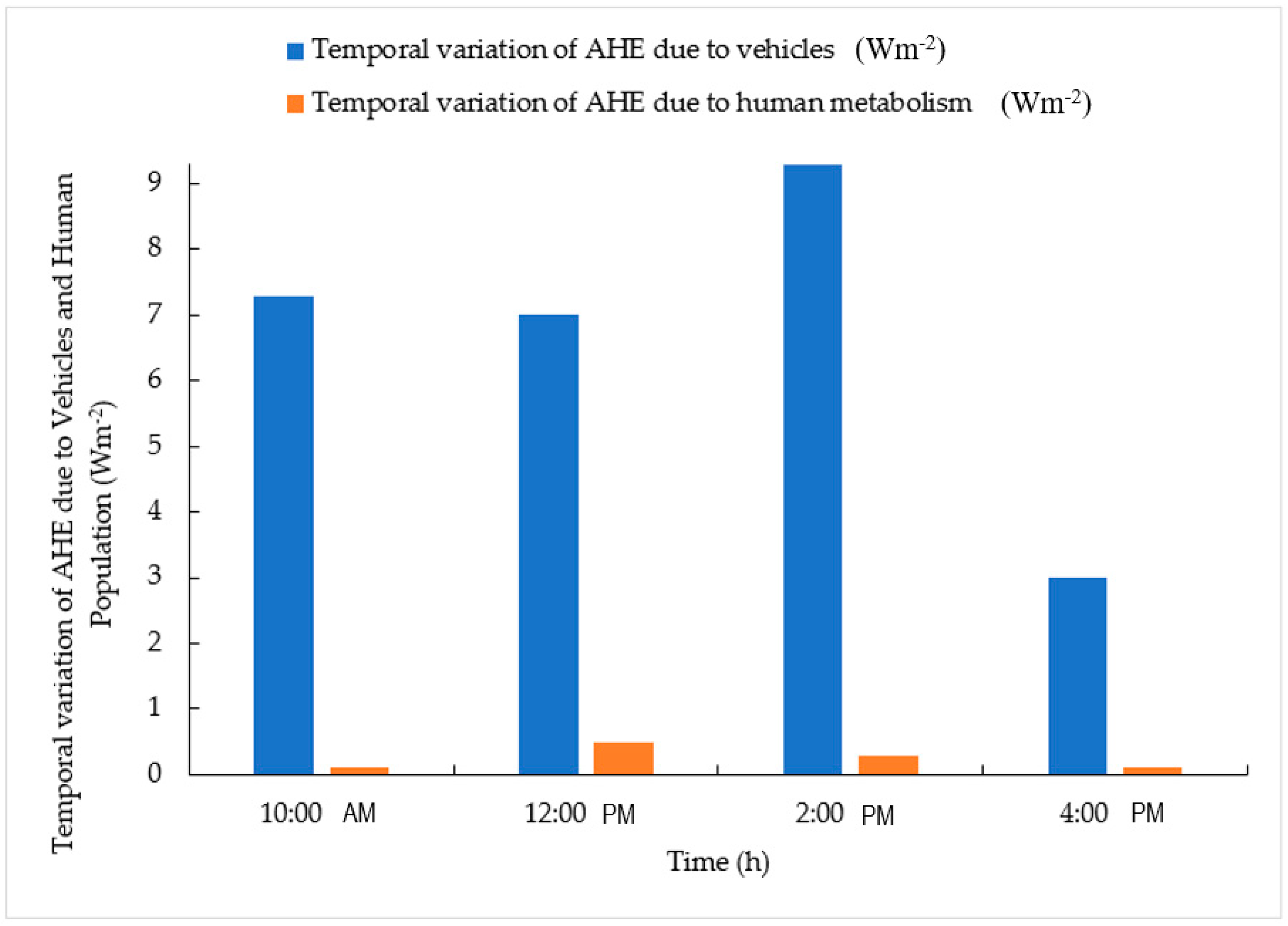
2.4.1. Estimation of Anthropogenic Heat Emission from Vehicle Traffic
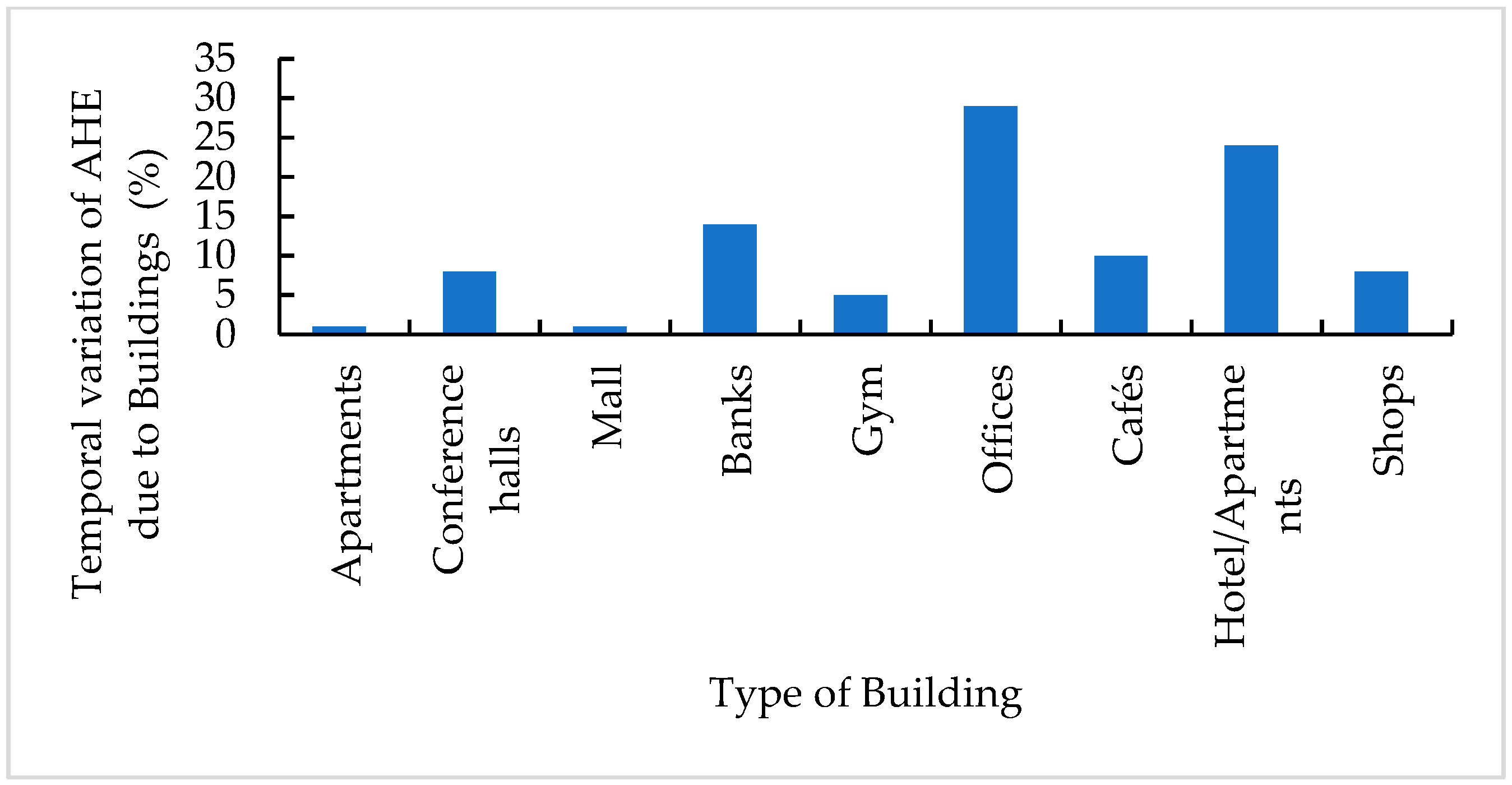
2.4.2. Estimation of Anthropogenic Heat Emission from Buildings
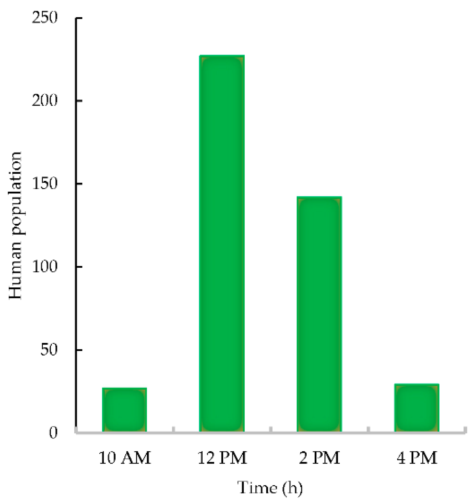
2.4.3. Estimation of Anthropogenic Heat Emission from Human Population (Metabolism)
3. Results and Discussion
3.1. Microclimate (Temperature and Humidity) Variations
3.2. Anthropogenic Heat Emission Effects
3.3. Temporal Variation of Anthropogenic Heat Emission and Its Influence on Urban Heat Island Effects
3.4. Comparison between the Impacts of Anthropogenic Heat Emission in Darwin with Some Major Cities
4. Conclusions
Author Contributions
Funding
Institutional Review Board Statement
Informed Consent Statement
Conflicts of Interest
References
- United Nations. World Urbanization Prospects, Demographic Research. 2018. Available online: https://population.un.org/wup/publications/Files/WUP2018-Report.pdf (accessed on 4 April 2022).
- Stewart, D.P. The United Nations and Human Rights. A Critical Appraisal. Edited by Philip Alston. New York, Oxford: Oxford University Press, 1992. Pp. xiii, 748. Index. $145. Am. J. Int. Law 1994, 88, 386–388. [Google Scholar] [CrossRef]
- Mishra, J.; Mishra, P.; Arora, N.K. Linkages between environmental issues and zoonotic diseases: With reference to COVID-19 pandemic. Environ. Sustain. 2021, 4, 455–467. [Google Scholar] [CrossRef]
- Li, G.; Zhang, X.; Mirzaei, P.A.; Zhang, J.; Zhao, Z. Urban heat island effect of a typical valley city in China: Responds to the global warming and rapid urbanization. Sustain. Cities Soc. 2018, 38, 736–745. [Google Scholar] [CrossRef]
- Nath, B.; Ni-Meister, W.; Choudhury, R. Impact of urbanization on land use and land cover change in Guwahati city, India and its implication on declining groundwater level. Groundw. Sustain. Dev. 2021, 12, 100500. [Google Scholar] [CrossRef]
- Huang, L.; Zhai, J.; Sun, C.Y.; Liu, J.Y.; Ning, J.; Zhao, G.S. Biogeophysical Forcing of Land-Use Changes on Local Temperatures across Different Climate Regimes in China. J. Clim. 2018, 31, 7053–7068. [Google Scholar] [CrossRef]
- Luo, X.; Vahmani, P.; Hong, T.; Jones, A. City-Scale Building Anthropogenic Heating during Heat Waves. Atmosphere 2020, 11, 1206. [Google Scholar] [CrossRef]
- Mirzaei, P.A.; Haghighat, F. Approaches to study Urban Heat Island–Abilities and limitations. Build. Environ. 2010, 45, 2192–2201. [Google Scholar] [CrossRef]
- Mazzone, A. Thermal comfort and cooling strategies in the Brazilian Amazon. An assessment of the concept of fuel poverty in tropical climates. Energy Policy 2020, 139, 111256. [Google Scholar] [CrossRef]
- FAN, H.; SAILOR, D. Modeling the impacts of anthropogenic heating on the urban climate of Philadelphia: A comparison of implementations in two PBL schemes. Atmos. Environ. 2005, 39, 73–84. [Google Scholar] [CrossRef]
- Lu, Y.; Yue, W.; Huang, Y. Effects of Land Use on Land Surface Temperature: A Case Study of Wuhan, China. Int. J. Environ. Res. Public Health 2021, 18, 9987. [Google Scholar] [CrossRef]
- Lung, S.-C.C.; Thi Hien, T.; Cambaliza, M.O.L.; Hlaing, O.M.T.; Oanh, N.T.K.; Latif, M.T.; Lestari, P.; Salam, A.; Lee, S.-Y.; Wang, W.-C.V.; et al. Research Priorities of Applying Low-Cost PM2.5 Sensors in Southeast Asian Countries. Int. J. Environ. Res. Public Health 2022, 19, 1522. [Google Scholar] [CrossRef] [PubMed]
- Doan, V.Q.; Kusaka, H.; Nguyen, T.M. Roles of past, present, and future land use and anthropogenic heat release changes on urban heat island effects in Hanoi, Vietnam: Numerical experiments with a regional climate model. Sustain. Cities Soc. 2019, 47, 101479. [Google Scholar] [CrossRef]
- Chen, B.; Wu, C.; Liu, X.; Chen, L.; Wu, J.; Yang, H.; Luo, T.; Wu, X.; Jiang, Y.; Jiang, L.; et al. Seasonal climatic effects and feedbacks of anthropogenic heat release due to global energy consumption with CAM5. Clim. Dyn. 2019, 52, 6377–6390. [Google Scholar] [CrossRef]
- Yang, Y.; Ren, L.; Li, H.; Wang, H.; Wang, P.; Chen, L.; Yue, X.; Liao, H. Fast Climate Responses to Aerosol Emission Reductions During the COVID-19 Pandemic. Geophys. Res. Lett. 2020, 47, e2020GL089788. [Google Scholar] [CrossRef]
- Chapman, S.; Watson, J.; McAlpine, C. Large seasonal and diurnal anthropogenic heat flux across four Australian cities. J. South. Hemisph. Earth Syst. Sci. 2016, 66, 342–360. [Google Scholar] [CrossRef]
- Azizalrahman, H.; Hasyimi, V. A model for urban sector drivers of carbon emissions. Sustain. Cities Soc. 2019, 44, 46–55. [Google Scholar] [CrossRef]
- de Almeida, C.R.; Teodoro, A.C.; Gonçalves, A. Study of the Urban Heat Island (UHI) Using Remote Sensing Data/Techniques: A Systematic Review. Environments 2021, 8, 105. [Google Scholar] [CrossRef]
- Chen, S.; Hu, D. Parameterizing anthropogenic heat flux with an energy-consumption inventory and multi-source remote sensing data. Remote Sens. 2017, 9, 1165. [Google Scholar] [CrossRef] [Green Version]
- Zheng, Y.; Weng, Q. High spatial- and temporal-resolution anthropogenic heat discharge estimation in Los Angeles County, California. J. Environ. Manag. 2018, 206, 1274–1286. [Google Scholar] [CrossRef]
- Lu, Y.; Wang, Q.; Zhang, Y.; Sun, P.; Qian, Y. An estimate of anthropogenic heat emissions in China. Int. J. Climatol. 2016, 36, 1134–1142. [Google Scholar] [CrossRef] [Green Version]
- Sun, R.; Wang, Y.; Chen, L. A distributed model for quantifying temporal-spatial patterns of anthropogenic heat based on energy consumption. J. Clean. Prod. 2018, 170, 601–609. [Google Scholar] [CrossRef]
- Ross, J.; Cunningham, C.O.; Hanna, D.B. HIV outcomes among migrants from low-income and middle-income countries living in high-income countries. Curr. Opin. Infect. Dis. 2018, 31, 25–32. [Google Scholar] [CrossRef] [PubMed]
- Bohnenstengel, S.I.; Hamilton, I.; Davies, M.; Belcher, S.E. Impact of anthropogenic heat emissions on London’s temperatures. Q. J. R. Meteorol. Soc. 2014, 140, 687–698. [Google Scholar] [CrossRef]
- World Bank Country and Lending Groups. Available online: https://datahelpdesk.worldbank.org/knowledgebase/articles/906519 (accessed on 11 February 2022).
- Australian Government Bureau of Meteorology. Climate Statistics for Australian Locations. Available online: http://www.bom.gov.au/climate/averages/tables/cw_014015.shtml (accessed on 11 February 2022).
- Yang, W.; Chen, B.; Cui, X. High-Resolution Mapping of Anthropogenic Heat in China from 1992 to 2010. Int. J. Environ. Res. Public Health 2014, 11, 4066–4077. [Google Scholar] [CrossRef] [PubMed] [Green Version]
- Australian Institute of Refrigeration Air Conditioning and Heating (AIRAH). Thought Leadership Policy and Advocacy Positions 2017–2020; Australian Institute of Refrigeration Air Conditioning and Heating (AIRAH): Melbourne, Australia, 2020. [Google Scholar]
- Northern Territory Planning Commission; Central Darwin Area Plan. Central Darwin Area Plan in NT Planning Scheme. 2021. Available online: https://planningcommission.nt.gov.au/projects/central-darwin-area-plan (accessed on 11 February 2022).
- Afshari, A.; Schuch, F.; Marpu, P. Estimation of the traffic related anthropogenic heat release using BTEX measurements—A case study in Abu Dhabi. Urban Clim. 2018, 24, 311–325. [Google Scholar] [CrossRef]
- Wang, S.; Hu, D.; Yu, C.; Chen, S.; Di, Y. Mapping China’s time-series anthropogenic heat flux with inventory method and multi-source remotely sensed data. Sci. Total. Environ. 2020, 734, 139457. [Google Scholar] [CrossRef]
- Wang, K.; Aktas, Y.D.; Malki-Epshtein, L.; Wu, D.; Ammar Bin Abdullah, M.F. Mapping the city scale anthropogenic heat emissions from buildings in Kuala Lumpur through a top-down and a bottom-up approach. Sustain. Cities Soc. 2022, 76, 103443. [Google Scholar] [CrossRef]
- Smith, C.; Lindley, S.; Levermore, G. Estimating spatial and temporal patterns of urban anthropogenic heat fluxes for UK cities: The case of Manchester. Theor. Appl. Climatol. 2009, 98, 19–35. [Google Scholar] [CrossRef]
- Karim, M.A.; Hasan, M.M.; Khan, M.I.H. A simplistic and efficient method of estimating air-conditioning load of commercial buildings in the sub-tropical climate. Energy Build. 2019, 203, 109396. [Google Scholar] [CrossRef]
- Daniel, L. ‘We like to live in the weather’: Cooling practices in naturally ventilated dwellings in Darwin, Australia. Energy Build. 2018, 158, 549–557. [Google Scholar] [CrossRef]
- Yang, W.; Wong, N.H.; Jusuf, S.K. Thermal comfort in outdoor urban spaces in Singapore. Build. Environ. 2013, 59, 426–435. [Google Scholar] [CrossRef]
- Mohammad Harmay, N.S.; Kim, D.; Choi, M. Urban Heat Island associated with Land Use/Land Cover and climate variations in Melbourne, Australia. Sustain. Cities Soc. 2021, 69, 102861. [Google Scholar] [CrossRef]
- Moriwaki, R.; Kanda, M.; Senoo, H.; Hagishima, A.; Kinouchi, T. Anthropogenic water vapor emissions in Tokyo. Water Resour. Res. 2008, 44, 11. [Google Scholar] [CrossRef]
- Adelia, A.S.; Yuan, C.; Liu, L.; Shan, R.Q. Effects of urban morphology on anthropogenic heat dispersion in tropical high-density residential areas. Energy Build. 2019, 186, 368–383. [Google Scholar] [CrossRef]
- Pigeon, G.; Legain, D.; Durand, P.; Masson, V. Anthropogenic heat release in an old European agglomeration (Toulouse, France). Int. J. Climatol. 2007, 27, 1969–1981. [Google Scholar] [CrossRef]
- Mostafavi, F.; Tahsildoost, M.; Zomorodian, Z. Energy efficiency and carbon emission in high-rise buildings: A review (2005-2020). Build. Environ. 2021, 206, 108329. [Google Scholar] [CrossRef]
- SMIC. Climate, Inadvertent Climate Modification: Report of the Study of Man’s Impact on Climate (SMIC); Study of Man’s Impact on Climate (SMIC); MIT Press: Cambridge, MA, USA, 1971. [Google Scholar]
- Hulley, G.C.; Dousset, B.; Kahn, B.H. Rising Trends in Heatwave Metrics Across Southern California. Earth’s Futur. 2020, 8, 7. [Google Scholar] [CrossRef]
- Dey, R.; Lewis, S.C.; Arblaster, J.M.; Abram, N.J. A review of past and projected changes in Australia’s rainfall. WIREs Clim. Chang. 2019, 10, 3. [Google Scholar] [CrossRef]
- Australian Building Codes Board. Climate Zone Map: Australia Wide. Aust. Build. Codes Board 2019, 1. Available online: https://www.abcb.gov.au/Resources/Tools-Calculators/Climate-Zone-Map-Australia-Wide# (accessed on 12 February 2022).
- de Jesus, A.L.; Thompson, H.; Knibbs, L.D.; Hanigan, I.; De Torres, L.; Fisher, G.; Berko, H.; Morawska, L. Two decades of trends in urban particulate matter concentrations across Australia. Environ. Res. 2020, 190, 110021. [Google Scholar] [CrossRef]
- Block, A.H.; Livesley, S.J.; Williams, N.S.G. Responding to the Urban Heat Island: A Review of the Potential of Green Infrastructure. Vic. Cent. Clim. Chang. Adapt. 2012, 1–62. Available online: http://staging.202020vision.com.au/media/1026/responding-to-the-urban-heat-island-a-review-of-the-potential-of-green-infrastructure.pdf (accessed on 12 February 2022).
- Ali, M.M.; Al-Kodmany, K. Tall Buildings and Urban Habitat of the 21st Century: A Global Perspective. Buildings 2012, 2, 384–423. [Google Scholar] [CrossRef] [Green Version]
- Douglas, A.N.J.; Morgan, A.L.; Rogers, E.I.E.; Irga, P.J.; Torpy, F.R. Evaluating and comparing the green wall retrofit suitability across major Australian cities. J. Environ. Manag. 2021, 298, 113417. [Google Scholar] [CrossRef] [PubMed]
- Slavko, B.; Glavatskiy, K.; Prokopenko, M. City structure shapes directional resettlement flows in Australia. Sci. Rep. 2020, 10, 8235. [Google Scholar] [CrossRef] [PubMed]
- Newcombe, K. Energy use in Hong Kong: Part III, spatial and temporal patterns. Urban Ecol. 1976, 2, 139–172. [Google Scholar] [CrossRef]


| Year | City | QAHE (Wm−2) | Reference | ||||
|---|---|---|---|---|---|---|---|
| Annual | Winter | Autumn | Summer | Spring | |||
| 1970 | Moscow, Russia | 127 | |||||
| 1971 | Hong Kong, China | 33 | 41 | 32 | [42] | ||
| 1986–1994 | Ginza, Tokyo | 86 a | [51] | ||||
| 1986–1994 | Shinjuku, Tokyo | 136 a | [38] | ||||
| 2005 | Toulouse, France | 100 | 25 | [38] | |||
| 2008 | Manchester, England | 23 | [40] | ||||
| 2011 | Singapore | 113 a | [33] | ||||
| 2016 | Melbourne, Australia | 376 | [51] | ||||
| 2016 | Brisbane, Australia | 261 | [16] | ||||
| 2016 | Sydney, Australia | 256 | [16] | ||||
| 2016 | Adelaide, Australia | 39 | [16] | ||||
| 2017 | Los Angeles, USA | 100 | [16] | ||||
| 2017 | Beijing, China | 135 | 84 | 82 | 77 | [20] | |
| 2021 | Darwin | 121 a | Present study | ||||
Publisher’s Note: MDPI stays neutral with regard to jurisdictional claims in published maps and institutional affiliations. |
© 2022 by the authors. Licensee MDPI, Basel, Switzerland. This article is an open access article distributed under the terms and conditions of the Creative Commons Attribution (CC BY) license (https://creativecommons.org/licenses/by/4.0/).
Share and Cite
Rajapaksha, S.; Nnachi, R.C.; Tariq, M.A.U.R.; Ng, A.W.M.; Abid, M.M.; Sidiqui, P.; Rais, M.F.; Aamir, E.; Herrera Diaz, L.; Kimiaei, S.; et al. An Estimation of the Anthropogenic Heat Emissions in Darwin City Using Urban Microclimate Simulations. Sustainability 2022, 14, 5218. https://doi.org/10.3390/su14095218
Rajapaksha S, Nnachi RC, Tariq MAUR, Ng AWM, Abid MM, Sidiqui P, Rais MF, Aamir E, Herrera Diaz L, Kimiaei S, et al. An Estimation of the Anthropogenic Heat Emissions in Darwin City Using Urban Microclimate Simulations. Sustainability. 2022; 14(9):5218. https://doi.org/10.3390/su14095218
Chicago/Turabian StyleRajapaksha, Shehani, Raphael Chukwuka Nnachi, Muhammad Atiq Ur Rehman Tariq, Anne W. M. Ng, Malik Muneeb Abid, Paras Sidiqui, Muhammad Farooq Rais, Erum Aamir, Luis Herrera Diaz, Saeed Kimiaei, and et al. 2022. "An Estimation of the Anthropogenic Heat Emissions in Darwin City Using Urban Microclimate Simulations" Sustainability 14, no. 9: 5218. https://doi.org/10.3390/su14095218