Analysis of Landscape Change and Its Driving Mechanism in Chagan Lake National Nature Reserve

Abstract

Lake ecosystems play an important role in regional ecological security and the sustainable development of the economy and society. In order to study the evolution of landscape patterns and the main driving forces in the Chagan Lake Nature Reserve in recent years, we used landscape type data from 2005, 2010, 2015, and 2019 to study the characteristics of the regional landscape’s structural changes. At the same time, the spatial heterogeneity of the driving factors of landscape change was analyzed using the spatial analysis method, and the driving mechanism of landscape change was quantitatively analyzed. The results showed that: (1) from 2005 to 2019, the area of cultivated land, marshland, and water bodies increased, while the area of grassland and the area of bare land decreased. (2) The dominant patch types in the study area formed good connectivity, and the degree of landscape fragmentation increased. (3) In the past 15 years, there has been spatial heterogeneity in the regression coefficients of different driving factors of landscape change: the area with a greater influence of the elevation factor was in the south; the regression coefficient of precipitation showed the spatial distribution characteristics of highs in the west and lows in the east; the gross domestic product had a greater impact on the east and the south; the spatial variation of grain yield was mainly reflected in the southeast and northwest regions; the fishery yield gradually changed from high in the southeast and low in the northwest to the distribution characteristic of decreasing from the east to the southwest; the lake fluorine content showed a distribution pattern that gradually changed from high in the southeast and low in the northwest to high in the middle and low in the north and south; the distribution pattern of the distance to oil production changed from north to southeast to south to north; the distance to the road changed from high in the east and low in the west to the opposite spatial distribution pattern. (4) The interaction of precipitation and lake fluoride content with other factors showed a strong driving effect, which had a significant impact on the landscape change of Chagan Lake Nature Reserve. Since the study area is located in a typical fluorine-rich geochemical environment, human activities, such as the expansion of irrigation areas around Chagan Lake and groundwater exploitation, have accelerated the dissolution of fluorine-containing minerals, promoted the enrichment process of fluorine in Chagan Lake, and enhanced the explanatory power of lake fluorine content in terms of landscape changes. At the same time, the increase in precipitation during the study period is beneficial to the growth of vegetation and the storage of water in lakes, which promotes changes in landscape types such as grasslands and areas of water.

1. Introduction

As an important part of global water resources, lakes play a key role in water conservation, water quality purification, flood storage, drought prevention, climate regulation, biodiversity maintenance, and providing production and living water resources [1]; they become more and more critical in supporting the sustainable economic development of a region, a country, and even the world. Unfortunately, in recent years, many lakes and reservoirs have shown a trend of serious deterioration. Human activities, in addition to the overall climate changes, are causing more threats to the balance of the water cycle, such as landscape fragmentation, urbanization, industry, aquaculture, biological invasion, and water resource depletion, which have seriously affected the sustainable development of lakes and the surrounding areas. Studies have shown that pollutants in the Great Lakes of the United States are related to the impact of urban land cover and wastewater discharge [2], while land-cover change is mainly influenced by current land use, human habitation, industry, and demographic change [3]. Eutrophication in Taihu Lake in China is mainly caused by agricultural non-point source pollution, domestic sewage discharge, industrial wastewater discharge, and atmospheric deposition [4]; the area of algal blooms caused by eutrophication has notable correlations with the sunshine duration, wind speed and direction, precipitation, and air pressure [5]. An in-depth understanding of the impact of different factors on the lake environment will help policymakers to adopt targeted sustainable development management and policies to maintain the long-term beneficial properties of lakes.

Remote sensing and geographic information systems (GIS) are useful tools for monitoring and understanding the changing trends of lakes and their surrounding ecosystems. Multispectral satellite imagery is an important source of landscape information [6]. In recent years, many scholars have conducted research on lakes, such as the dynamic change characteristics of landscape patterns [7,8,9], ecosystem service value [10,11], the driving factors of landscape change [12,13], and dynamic landscape simulation and prediction [14,15].

Previous studies on the driving factors of ecosystem changes mostly used models to quantitatively analyze the driving strength of single factors according to their dependent variables, such as: gray correlation [16,17], principal component analysis [18,19,20], and Pearson correlation analysis [21]. Traditional statistical analytical models have a guiding role in quantitatively explaining the factors of landscape changes, but they cannot reflect the unique spatial heterogeneity of the geographic phenomena. Therefore, it is necessary to eliminate the effects of the correlation among the independent variables (multicollinearity) and to identify the relationship between multiple factors, such as whether there is an interaction between the two factors, and the strength and direction, either linear or nonlinear, of the interaction. This paper proposes a method to analyze the driving mechanism of landscape change, which can not only eliminate the multicollinearity between factors and reflect the spatial heterogeneity of each driving factor [22,23] but also better realize the detection of driving factors and evaluate whether the driving force of landscape change will be increased or weakened when the driving factors work together, as well as whether the effects of these factors are independent of each other [24,25,26,27], so as to better reveal the driving mechanisms of the landscape pattern changes.

Chagan Lake, located in the middle of northeast China, is an important breeding and resting place for migratory birds along the East Asia–Australia migratory bird migration route. It plays an important role in the protection of global and national biodiversity, especially in terms of the conservation of rare and endangered birds. Chagan Lake is an important part of the North China Nature Reserve Group and an important ecological barrier in the western region of Jilin Province. Approved as a national nature reserve in 2007, Chagan Lake has a unique ecosystem structure of prairie lakes, surrounded by scattered rivers, smaller lakes, marshes, and wetlands. The ecosystem types are diverse. They play an important role in regulating and storing river runoff, providing water sources, flood control, and aquaculture, maintaining biodiversity and basin ecological environment security. The Songnen Plain, where Chagan Lake is located, is surrounded by volcanic rocks, secondary volcanic rocks, and fluorite veins, constituting a typical fluorine-rich geochemical environment zone [28]. In recent years, due to the development of tourism in the reserve, agricultural production has shifted from animal husbandry to planting, and with interference from human activities such as oil exploitation, the landscape pattern of Chagan Lake Nature Reserve is constantly changing. At the same time, human activities such as the expansion of the irrigation area around Chagan Lake, the construction of the river–lake connection project in western Jilin, and the exploitation of groundwater have changed the original hydrological and water-quality environment, resulting in the increase of fluoride content in the lake and hidden dangers in terms of regional water environment safety. Understanding the characteristics and main driving forces of the landscape changes in Chagan Lake can help to carry out better protection and management of the lake, which has an important guiding role in improving the regional ecological environment and economic development. Our predecessors have conducted much research on the Chagan Lake area, but this has mostly focused on the water quality characteristics of Chagan Lake [29,30], water environment change [31,32], the groundwater environment [33,34], and pollutant distribution [35]; for example, Wang Fengyan [36] determined and compared the surface deformation of three typical land cover types in Chagan Lake, and analyzed the influencing factors of the lakeside areas. However, more of the driving factors for landscape change in the Chagan Lake Nature Reserve need to be studied.

This study takes Chagan Lake National Nature Reserve as the research area and explores the degree of change of different landscape types under natural and human disturbances, based on the changes in landscape types and landscape patterns in the past 15 years. We aim to answer the following questions. How has the landscape type of Chagan Lake Nature Reserve changed during the study period? What are the factors driving the change and how do they drive that change? What does this teach us about the lake’s landscape changes, generally? The results of this paper show that: the area with the greatest influence from the elevation factor was in the south, where the terrain is higher; the annual precipitation in the west was higher, and the precipitation had a greater impact on the landscape changes in the west; the growth of the gross domestic product(GDP) promotes the transformation of bare land into cultivated land; the reduction of food production will prompt people to expand cultivated land area, compete for the lake’s water supply, and accelerate the changes of landscape types; the development of aquaculture will lead to the shrinking of lakes; the expansion of irrigation areas around Chagan Lake will promote the enrichment of fluoride in Chagan Lake and enhance the explanatory power of lake fluorine content in terms of landscape change; the development of oil fields occupies much space and destroys the original landform, leading to changes in landscape types; the expansion of road networks is often accompanied by economic development, which has an impact on the surrounding landscape types. In addition, we found that precipitation and the lake fluoride content have a greater impact on landscape changes in the study area. This is because the annual precipitation increases year by year during the study period, which is conducive to the growth of vegetation and lake water storage. At the same time, the study area is located in a typical fluorine-rich geochemical environment. Human activities, such as the expansion of irrigation areas around Chagan Lake, have changed the original hydrological and water-quality environment and promoted the enrichment process of fluorine in Chagan Lake, increasing the explanatory power of lake fluorine content. Before proposing lake protection policies, it is necessary to conduct a comprehensive investigation of its resources, improve the level of modern management, and realize scientific decision-making on the management and protection of Chagan Lake. In addition, the restoration and protection of the lake require continued attention from the government and the public.

This paper is composed of five sections. Section 1 comprises the introduction, followed by an explanation of the materials and methods in Section 2. Section 3 introduces the results of changes in landscape patterns and analyzes the spatial heterogeneity of each factor’s impact on landscape change. Section 4 discusses the driving mechanisms of these factors and the implications for lake conservation and management. Section 5 offers our conclusions in the final section.

2. Materials and Methods

2.1. Study Area

The study area of Chagan Lake is located at 45°05′42″–45°25′50″ N and 124°03′28″–124°30′59″ E, situated in the northwest of Jilin Province in northeast China and at the junction of the Huolin River and the Nen River. The main body of the study area is in the Qianguoerluosi Mongolian Autonomous County of Songyuan City, partly located in the Da’an City of Baicheng and Qian’an County of Songyuan, with a total area of 647 km². The main bottom landform features of the lake are low and flat with slight ups and downs, higher in the southeast, slightly higher in the southwest, and lower in the middle and northeast. The terrain in Dongchuantou, Xichuantou, and Qingshantou of the lake is relatively higher, with an elevation of 140–160 m above sea level. The terrain immediately surrounding the lake is low-lying, with secondary river terraces remaining beside the lake. Chagan Lake has several larger marshes with different water levels, and there are some sand dunes with a relative height of no more than 5 m. According to the area’s genesis and morphological characteristics, the landform of this area can be divided into an alluvial lake plain and a valley alluvial plain. The alluvial lake plain is located in the low-lying areas of the lake region, and the valley alluvial plain is distributed in the Huolin River valley and the ancient Nenjiang river channel (Figure 1).

The study area is located at the eastern edge of the mid-latitude Eurasian continent, belonging to a continental monsoon semi-arid area of the northern temperate zone. Affected by atmospheric circulation and under the control of cold and warm air masses, the annual climate changes in the four seasons are relatively obvious. Spring is dry and windy, summer is warm and less rainy, autumn is clear and refreshing, and winter is severely cold and very long. There is a substantial temperature difference between cold periods and heat in a year, and the spring and autumn seasons are relatively short. The multi-year average temperature of the region is 4.5 °C, the average annual precipitation is 379 mm, and the annual average evaporation is 948 mm. Winter is from 30 September to 3 May of the following year, accounting for 60% of the whole year. The annual freezing period of the lake surface is 130 days, the annual frost-free period is about 160 days, and the maximum frozen soil depth is 2.04 m.

The production in the reserve is mainly from fishing, and the tourism industry has developed rapidly. The farmers in the surrounding villages are mainly engaged in planting and food production, mainly of corn, rice, and other food crops.

According to the Chinese Program for Natural Protection, the core area is the well-preserved natural ecosystem and the concentrated distribution at the center is of rare and endangered animals and plants. Mass passage through the area and tourism activities are prohibited, and scientific research is generally not allowed. The buffer zone allows non-destructive scientific research and specimen collection activities, teaching activities, but, generally, no tourism activities. The scope of each protected area is shown in Figure 1c.

2.2. Data Sources

The remote sensing images used in this article are obtained from the website of the United States Geological Survey (http://www.usgs.gov/, accessed on 30 August 2020). The 2005, 2010, and 2015 datasets are of Landsat ETM images, and the 2019 set is of Landsat OLI images, with a spatial resolution of 30 m × 30 m; meteorological data, such as precipitation and evaporation, are obtained from the China Meteorological Data Network (http://data.cma.cn, accessed on 30 August 2020); socio-economic data, such as GDP, grain output, and the tourism comprehensive income are derived from the “Songyuan Statistical Yearbook” (https://navi.cnki.net, accessed on 30 August 2020); the monitoring data of fluorine content in Chagan Lake are from the Chagan Lake Governance and Protection Plan (2018–2030).

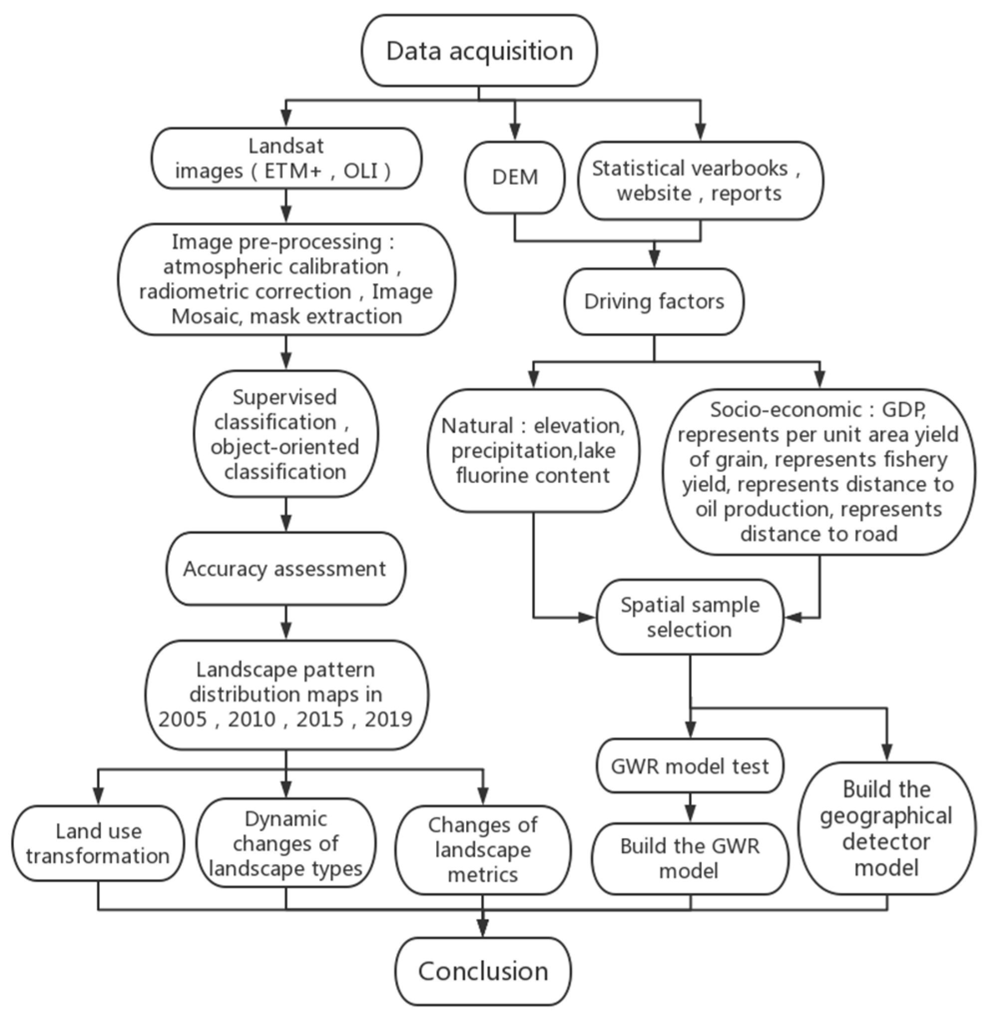
2.3. Process and Methods

The research process is shown in Figure 2.

2.3.1. Landscape Classification

Remote sensing images were preprocessed by atmospheric correction, geometric correction, Mosaic, and mask extraction, and were then interpreted on the Environment for Visualizing Images (ENVI) remote sensing image-processing platform. According to the land use of Chagan Lake, the landscape types of the study area were divided into five groups: cultivated land, grassland, water bodies, marshland, and bare land. The Landsat ETM images from 2005, 2010, and 2015 were classified using supervised classification [37], while the Landsat OLI images of 2019 were classified using an object-oriented classification method [38]. The landscape pattern distribution maps of the study area in four periods were obtained. The accuracy of the classification results was verified by a confusion matrix with uniformly selected test samples of Google Earth images. The kappa coefficients of 2005, 2010, 2015 and 2019 were 89.4%, 90.8%, 90.2% and 92.7%, respectively, meeting accuracy requirements.

2.3.2. Selection of Landscape Metrics

The landscape pattern index is a quantitative index employed to analyze heterogeneity at the landscape level using FRAGSTATS 4.0 [39]. In order to understand the characteristic changes to the landscape pattern in the study area, based on the ecological significance of each type of landscape index [40], this paper selected four indexes at both type level and landscape level; namely, patch density (PD), landscape shape index (LSI), Shannon diversity index (SHDI), and contagion index (CONTAG). On the basis of the landscape classification results, FRAGSTATS 4.2 was used to calculate on both the type and landscape scales, and the landscape pattern index for 4 years is obtained.

2.3.3. Land-Use Transfer Matrix

The land-use transfer matrix is the application of the Markov model to land-use change, which can quantitatively explain the mutual conversion between different land-use types, as well as the characteristics of the transfer ratio and the rate between different land types [41,42,43]. The calculation formula for the Markov transition matrix model is as follows:

$$\mathrm{S}=\left[\begin{array}{ccc}{\mathrm{S}}_{11}& \cdots & {\mathrm{S}}_{1\mathrm{n}}\\ ⋮& \ddots & ⋮\\ {\mathrm{S}}_{\mathrm{m}1}& \cdots & {\mathrm{S}}_{\mathrm{mn}}\end{array}\right]$$

(1)

where S_mn is the area transferred from land use type m to land-use type n during the study period; m represents the land use type code before transfer, n represents the land use type code after transfer, and m and n are equal to 5 as we only have five types of land use in the Chagan Lake land-use classification system. Based on the above calculation, we generated three transition matrixes and calculated the reduced and increased amount of each land-use type.

2.3.4. Selection of Driving Forces

According to the characteristics of the natural environment and development and construction of the Chagan Lake Nature Reserve, and considering the availability of data, 10 factors (natural factors: precipitation, elevation, evaporation, lake fluorine content; social factors: per unit-area yield of grain, GDP, comprehensive tourism income per area, fishery yield, distance to oil production, distance to the road) were selected for driving force analysis, and the multi-year average values of the corresponding driving factor data in the three time periods of 2005–2010, 2010–2015 and 2015–2019 were calculated. By using the interpolation analysis tool in ArcGIS 10.7, the corresponding indicators in the three time periods were assigned to the sample points of the study area as attribute data, to realize the spatialization of driving factors.

2.3.5. Analysis of Driving Factors, Based on Geographically Weighted Regression (GWR)

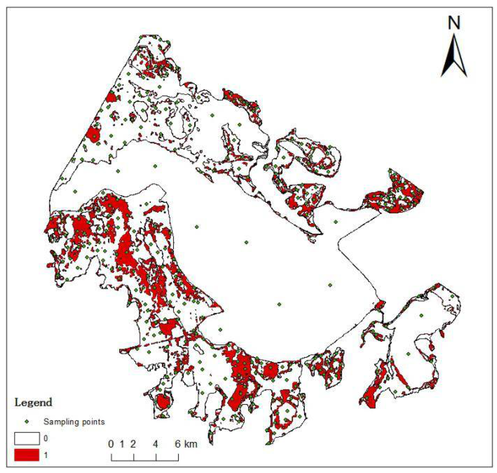
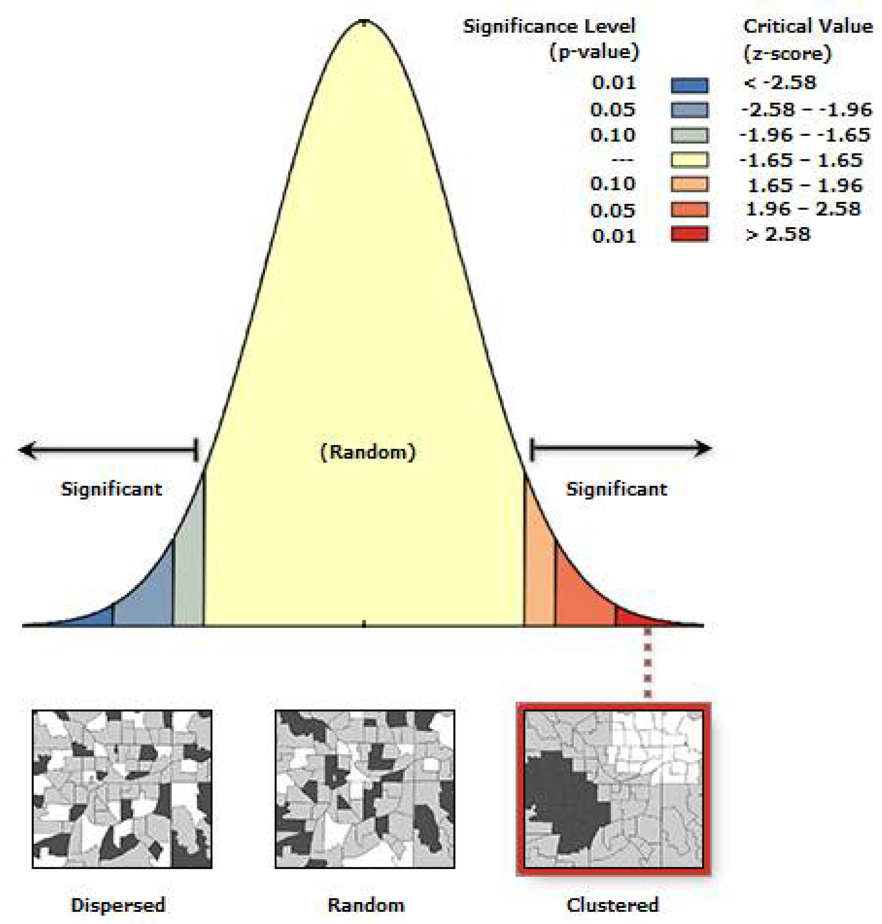
• Spatial sample selection

In order to realize the spatial modeling and analysis of driving factors, it was necessary to randomly select sample points within the study area and extract data. Based on the ArcGIS 10.7, the land-use maps of Chagan Lake Nature Reserve in 2005, 2010, 2015, and 2019 were spatially superimposed to obtain the three phases of the study area for the 2005–2010, 2010–2015, and 2015–2019 land-use change vector diagram; finally, the vector diagram was converted into raster images. Based on the raster images of land-use change, this paper used the ArcGIS “Create random points” tool to conduct random stratified sampling of areas with land use change (1) and unchanged (0) during the periods 2005–2010, 2010–2015, and 2015–2019. A total of 309 sample points took the vector; the number of points that were 0 and 1 was roughly the same, and the unequal sampling ratio would not affect the coefficient estimation of the explanatory variable in the model but would affect the constant term of the model. Using the ArcGIS “Extract multi values to points” function, the corresponding position information and driving force factor attribute value of 309 samples were extracted from the driving factor raster map. We took the vector map of land-use change from 2015 to 2019 as an example, and the sampling points are shown in Figure 3.

• GWR model test—ordinary least squares (OLS) regression

The prerequisite for applying the geographically weighted regression (GWR) model for analysis is that the variables have the characteristics of spatial autocorrelation. Therefore, before constructing the GWR model, the Moran I module in the ArcGIS software is used to test the spatial correlation of the dependent variables. The Moran I indices of the changes in landscape types from 2005 to 2010, 2010 to 2015, and 2015 to 2019 are calculated to be 0.132, 0.117, and 0.075, respectively. The Z values of the state statistics are 6.507, 5.762, and 3.749, and the p-values are all 0.000, respectively, indicating that the spatial distribution of landscape change in the study area has significant clustering characteristics and that there is a positive correlation (Figure 4). Therefore, it is necessary and feasible to use the GWR model to analyze the influencing factors of cultivated land area per capita.

In order to verify the applicability of the GWR model, OLS regression is used to test multicollinearity before the GWR, to ensure the accuracy of the model. The formula is:

$${\mathrm{y}}_{\mathrm{i}}={\beta }_0+{\displaystyle \sum _{\mathrm{j}=1}^{\mathrm{k}}{\beta }_{\mathrm{j}}{x}_{\mathrm{ij}}+{\epsilon }_{\mathrm{i}}}$$

(2)

$${\mathrm{y}}_{\mathrm{i}}={\beta }_0\left({\mathrm{u}}_{\mathrm{i}},{\mathrm{v}}_{\mathrm{i}}\right)+{\displaystyle \sum _{\mathrm{j}=1}^{\mathrm{k}}{\beta }_{\mathrm{j}}}\left({\mathrm{u}}_{\mathrm{i}},{\mathrm{v}}_{\mathrm{i}}\right)x_{\mathrm{ij}}+{\epsilon }_{\mathrm{i}}$$

(3)

where x_i and y_i refer to the regression independent variable and dependent variable, respectively; ${\beta }_0$ and ${\beta }_0$(u_i,v_i) are the global and the i-th sample constant items, respectively; ${\beta }_{\mathrm{j}}$(u_i,v_i) refers to the regression coefficient of the j-th parameter of the i-th sample, which reflects the spatial differentiation of the influence of different parameters on the sample. The positive and negative signs of the coefficient indicate the positive and negative correlation properties between the parameter and the spatial position, and the magnitude indicates the strength of the correlation degree. (u_i,v_i) refers to the i-th sample space coordinates; x_ij refers to the j-th parameter value of the i-th sample; ε_i represents the random error term; k represents the number of independent variables.

The results show the variance inflation factor (VIF) value of the four driving factors: GDP, comprehensive tourism income per area, evaporation, and the distance to an oil production point. All values are greater than 7.5, indicating that the explanatory variables are redundant and the influencing factors have multicollinearity. Through principal component analysis, after removing the two redundant variables of evaporation and tourism comprehensive income per area, the least-squares method was employed. The results are shown in

Table 1. The regression results of the OLS model for the driving forces of land-use change (2005–2010).

Driving Forces	Coefficient	Standard Deviation	t	Robust_Pr	VIF
Elevation (EL)	0.001727	0.013251	0.130354	0.898822	1.291934
Precipitation (P)	3.649503	1.44684	2.522396	0.017974 *	6.575416
Gross Domestic Product (GDP)	−0.000011	0.000004	−2.690913	0.000011 *	5.239569
Grain yield (GY)	−0.010697	0.004044	−2.645524	0.000000 *	1.119108
Fishery yield (FY)	0.000281	0.000162	1.735454	0.013825 *	7.478522
Lake fluorine content (LFC)	−0.279368	0.184039	−1.517983	0.088338	4.040279
Distance to oil production (DOP)	0.000012	0.00008	−1.660495	0.102692	1.204025
Distance to road (DR)	−0.000028	0.000017	−1.660495	0.102692 *	1.204025
	Joint F-Statistic	Jarque-Bera	Koenker (BP)	Joint Wald Statistic
	6.152154	34.837705	65.896048	254.815411	0.000000 *

* next to a number indicates a statistically significant p-value (p < 0.01).

.

From Table 1, it can be seen that the variance inflation factor (VIF) values of the 8 explanatory variables are all less than 7.5, and there is no multicollinearity among the driving factors. The significance level of the overall parameters of each factor shows that each factor presents strong statistical significance, so the model is statistically significant. The Jarque–Bera value shows that the test is significant, the residuals do not obey the normal distribution, and the model fits one-sidedly. In order to improve the fitting degree, the GWR model is needed.

• GWR model formulation

The GWR model is a geographically oriented spatial modeling method, based on the principle of ordinary least squares [44]. It is a localized linear regression model that considers the spatial heterogeneity of variables. The sample location information is added to the regression parameters. The relationship between variables can vary with the change of spatial position, and the spatial non-stationarity is handled well [45,46]. The key to GWR regression lies in the spatial weight matrix, generally calculated by a Gaussian function. The expression is as follows:

$${\mathrm{w}}_{\mathrm{ij}}=\exp (-{(d_{\mathit{ij}}/b)}^2)$$

(4)

where w_ij is the observation weight at position i; d_ij is the distance between the regression point i and the data point j; b is the bandwidth, which represents the functional relationship between the weight and the distance.

2.3.6. Geographical Detector Model Formulation

The geographic detector is a statistical analysis method with geographic characteristics that can detect spatial differentiation and reveal the driving forces behind it [25]. In this paper, the driving force of land-use change in Chagan Lake Nature Reserve is quantitatively explained by using a geographic detector, while the factor detector and the interactive detector are used for analysis.

• The factor detector detects the spatial divergence of Y and the degree of explanation of factor X to the spatial divergence of attribute Y. Measured by the value q, the expression is as follows:

$$q=1-\frac{{\displaystyle \sum _{h-1}^L{N}_h{\sigma }_h{}^2}}{N{\sigma }^2}$$

(5)

where h = 1, …, L is the stratification of variable Y or factor X (that is, classification or partition); N_h and N are the number of samples in layer h and the whole area, respectively; σ_h² and σ² are the total variance of layer h and regional total variance, respectively.

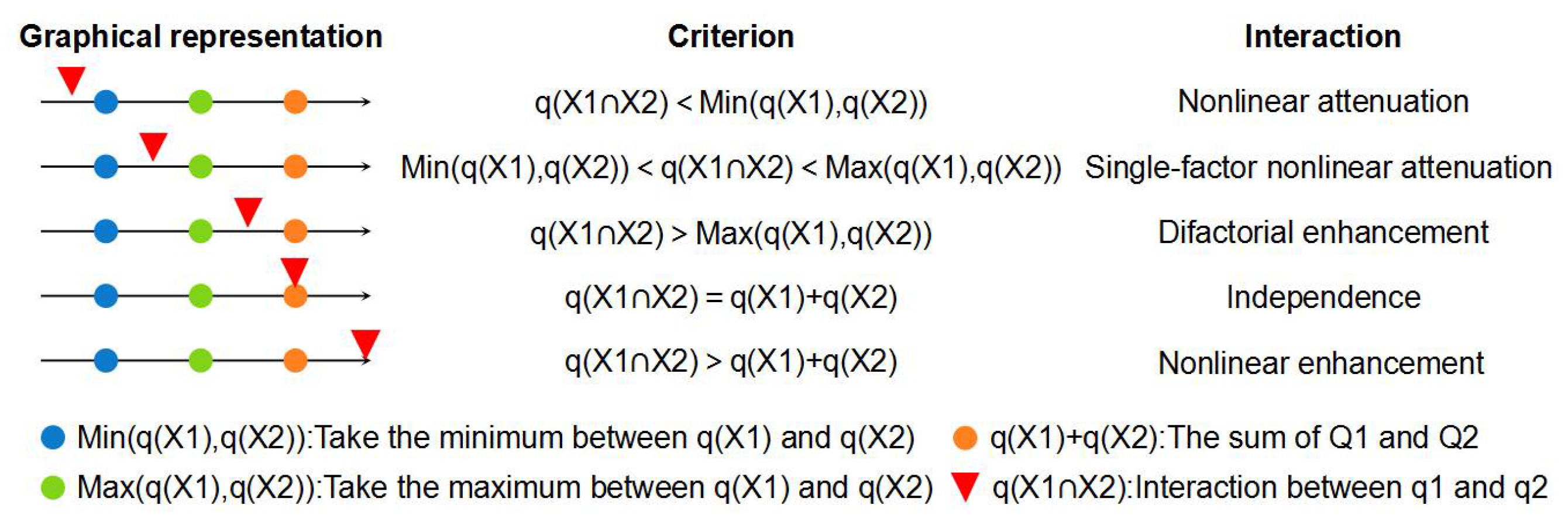
• The interactive detector evaluates the changes in the degree of interpretation of the combined effect of factors X1 and X2 relative to the single-factor effect. First, we calculate the interpretation degrees of two factors X1 and X2 for Y: q(X1) and q(X2), then we calculate the interpretation degrees q(X1∩X2) when they interact, and finally, q(X1), q(X2) and q(X1∩X2) are compared. The types of interaction between the two factors are as follows (see Figure 5).

3. Results

3.1. Changes in Landscape Pattern

3.1.1. Dynamic Changes of Landscape Types

Through the interpretation and classification of the remote-sensing images of Chagan Lake Nature Reserve in 2005, 2010, 2015, and 2019, the dynamic changes of landscape types in the four periods of the study area were finally obtained (Figure 6). Using ArcGIS 10.7 to calculate the area of each landscape type in the four periods, the results are shown in Figure 6.

Combining Figure 6 and Figure 7, it can be seen that Chagan Lake Nature Reserve has the largest surface area, followed by grassland, which was distributed throughout the entire area. The distribution of cultivated land was relatively scattered, while bare land was concentrated in the southwest and south. From 2005 to 2019, the water bodies in the study area was recovering, but it was still less than that in 2005. Most of the water bodies that decreased was located in the north; the area of cultivated land and marshland increased by 42.8 km² and 39.3 km²; the area of bare land and grassland decreased by 41.2 km² and 13.8 m², respectively; the total area of water bodies and marshland increased, and the area of bare land decreased greatly.

3.1.2. Land-Use Transfer Matrix

The land-use type transfer matrix was calculated using ArcGIS 10.7, and the dynamic changes in land-use types from 2005 to 2019 were obtained via a statistical summary (

Table 2. Conversion matrix of land use from 2005 to 2019.

Period	Land Use Type	Unit	Grassland	Cultivated Land	Water Bodies	Bare Land	Marshland	Total
2005–2010	Grassland	km2	48.71	5.48	0.68	4.46	0.79	60.12
	Cultivated land	km2	4.02	20.26	0.11	0.97	0.06	25.42
	Water bodies	km2	1.56	0.00	304.67	0.28	0.67	307.18
	Bare land	km2	74.92	6.94	26.44	47.85	5.90	162.05
	Marshland	km2	2.27	0.06	34.61	0.01	55.35	92.30
	Total	km2	131.48	32.74	366.51	53.57	62.77	647.07
2010–2015	Grassland	km2	47.08	3.83	1.05	72.97	1.02	125.95
	Cultivated land	km2	6.63	21.43	0.33	22.36	0.65	51.40
	Water bodies	km2	0.04	0.02	298.70	8.97	28.52	336.25
	Bare land	km2	0.39	0.03	1.68	14.58	0.00	16.68
	Marshland	km2	5.98	0.11	5.42	43.17	62.11	116.79
	Total	km2	60.12	25.42	307.18	162.05	92.30	647.07
2015–2019	Grassland	km2	94.33	7.20	0.67	7.15	7.39	117.08
	Cultivated land	km2	23.93	39.53	1.00	1.27	9.87	75.93
	Water bodies	km2	1.02	0.53	325.64	1.65	10.76	340.07
	Bare land	km2	4.48	0.11	0.78	6.27	0.63	12.71
	Marshland	km2	1.74	3.32	7.70	0.26	87.71	101.28
	Total	km2	125.95	51.40	336.25	16.68	116.79	647.07

). The results showed that from 2005 to 2010, 16.6% of the water bodies was transferred to bare land and marshland. From 2010 to 2015, the landscape of bare land changed greatly. A large amount of bare land was converted into grassland (44.9%), 26.6% into marshland, and some into cultivated land (13.8%) and water bodies (5.5%). From 2015 to 2019, grassland was mainly transferred to cultivated land (19%), 60.3% of bare land was restored to grassland, cultivated land, and water bodies, while 23.97% of marshland was converted to cultivated land, water bodies, and grassland.

3.1.3. Changes in Landscape Metrics

According to

Table 3. Changes of landscape type indexes in Chagan Lake Nature Reserve from 2005 to 2019.

Year	PD (#·100 ha−1)	LSI	CONTAG (%)	SHDI
2005	1.5674	14.6818	61.0976	1.2754
2010	1.1142	13.1761	60.1488	1.3212
2015	1.787	13.8539	60.7797	1.2914
2019	0.7636	11.4509	99.8536	1.2902

, in the past 15 years, the PD of Chagan Lake Nature Reserve showed a trend of first decreasing, then increasing, then decreasing again. The LSI reflects the complexity of the patch shape in the landscape. The LSI in the study area decreased from 14.6818 in 2005 to 11.4509 in 2019, and the landscape patches showed a relatively regular trend. The CONTAG increased from 61.0976% to 99.8536%, indicating that the patch fragmentation of the Chagan Lake Nature Reserve decreased, and the connectivity increased. The SHDI showed a trend of increasing first, then decreasing, then generally increasing, with 2010 as the turning point, indicating that the land-use types and landscape heterogeneity increased, but the dominant landscape types were not significant.

3.2. Analysis of the Driving Factors of Landscape Change

The sample-point parameters calculated by the GWR model were spatially interpolated in ArcGIS, and the spatial autocorrelation test was performed. The result was random and passed the statistical test. The interpolation results are shown in Figure 8 and Figure 9. The positive and negative of the regression coefficient indicates the positive and negative impact of each factor on landscape change, and the absolute value of the regression coefficient indicates the degree of impact on landscape change. The regression coefficient from the local GWR clearly reveals the relationship between landscape change and driving factors in the study area. The positive and negative regression coefficients indicate the spatial non-stationary of the driving factors of landscape change.

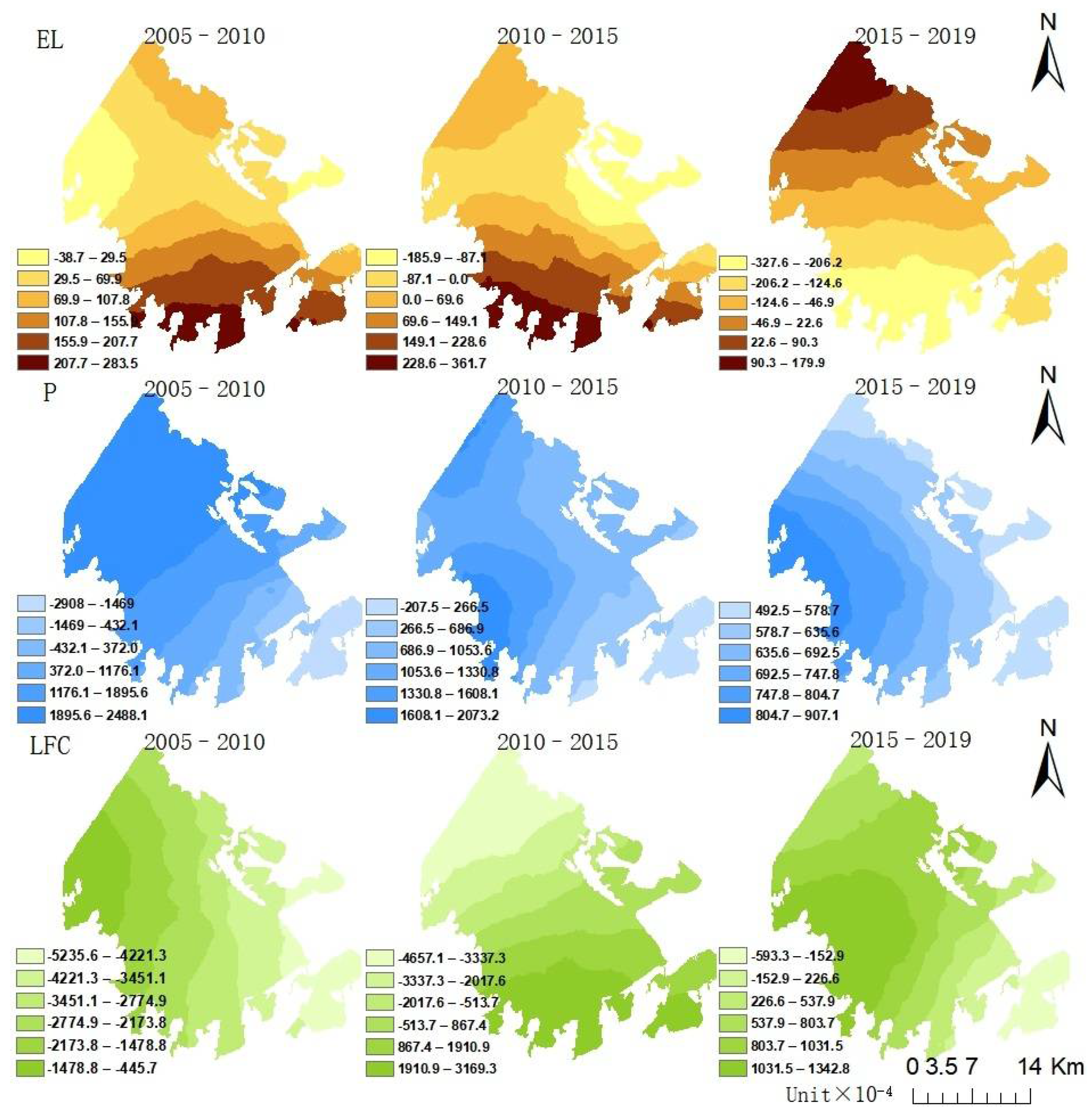
3.2.1. Spatial Heterogeneity Analysis of the Impact of Natural Factors on Landscape Change

Figure 8 showed the spatial distribution of the regression coefficients of natural factors in the GWR model. Different elevations have different temperatures, humidity, solar radiation, wind speed, and human activity intensity, which have an impact on the vegetation growth in the region. The spatial distribution of elevation (EL) did not change significantly from 2005 to 2015, and the spatial-temporal difference was not apparent. The highest coefficient of EL was located in the south, showing a stronger influence of the natural environment there, which was related to the higher terrain in the southeast and southwest of the region. From 2015 to 2019, the regression coefficient of EL decreased and the influence intensity also decreased.

The annual precipitation in the study area increased year by year during the study period, which was beneficial to the growth of vegetation and lake-water storage. As can be seen from Figure 8, the regression coefficient of precipitation (P) was large, indicating that P had a strong impact on landscape changes, showing a spatial distribution pattern of high in the west and low in the east, which was related to the distribution trend of precipitation, decreasing from west to east. From 2005 to 2019, the coefficient of P slightly decreased, but it was still much higher than the other factors except for lake fluorine content. From 2005 to 2015, the impact of P on landscape change showed a difference between east and west, with a negative influence for the eastern region and a positive influence for the western region. From 2015 to 2019, it only showed a positive influence. From 2010 to 2019, the positive-value area increased, indicating that the influence of P on landscape change was enhanced.

The distribution of fluoride content in Chagan Lake is lower at the entrance of the lake and higher at the center of the lake than at the exit. During the study period, the concentration of fluorine content in the lake showed an upward trend. From 2005 to 2019, the lake fluorine content (LFC) in Chagan Lake showed a spatial distribution pattern that gradually changed from high in the southeast and low in the northwest to high in the middle and low in the north and south, while the positive value area of landscape change showed an expanding trend, indicating that the impact of LFC on landscape change was enhanced. From 2005 to 2019, the coefficient of LFC gradually decreased, which indicated that the impact of this factor on landscape change was weakened.

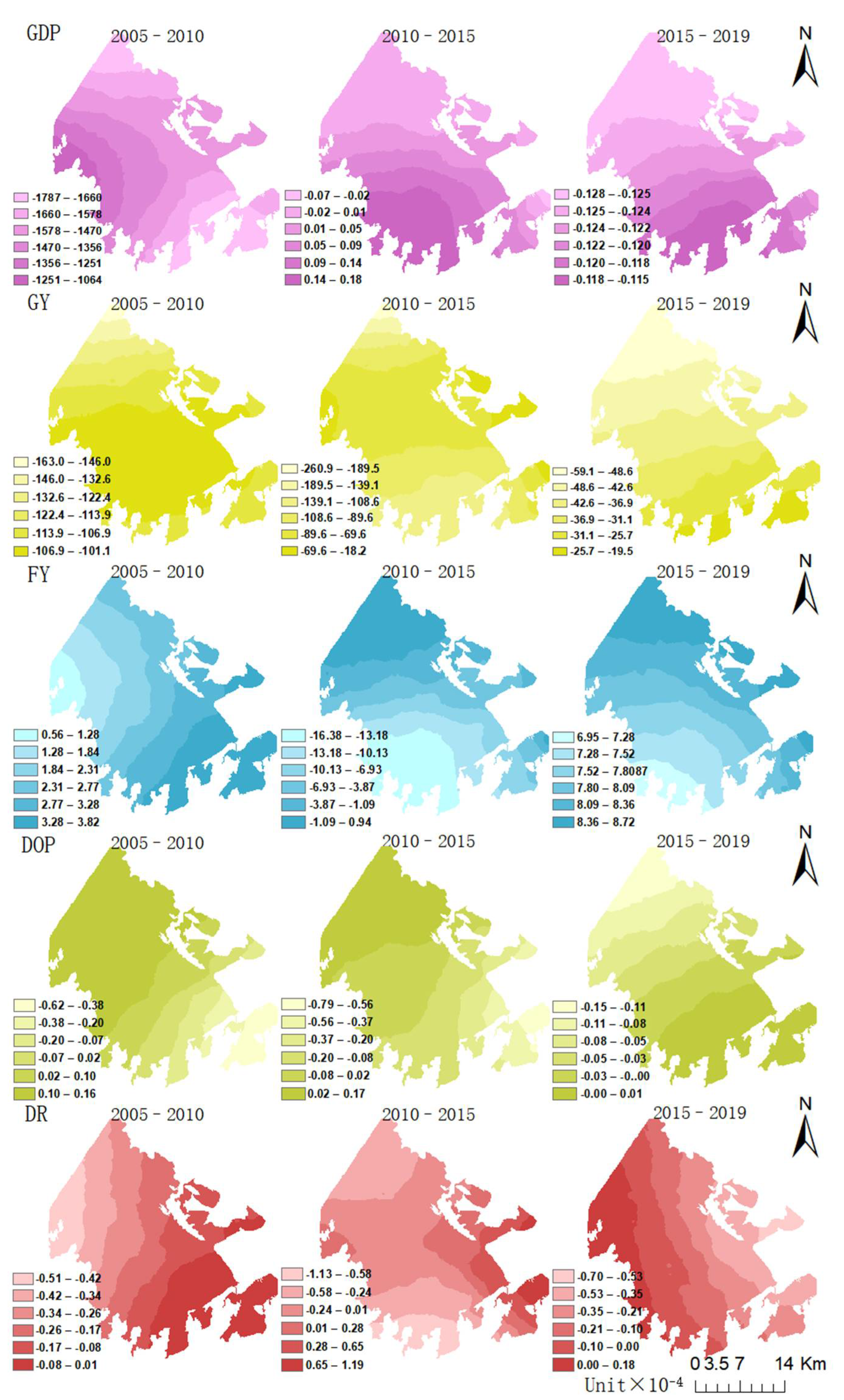
3.2.2. Spatial Heterogeneity Analysis of the Impact of Socio-Economic Factors on Landscape Change

Economic growth allows more bare land or water area to be occupied and reclaimed for specific land uses, to meet basic human needs [47]. As shown in Figure 9, the regression coefficient of gross domestic product (GDP) in the past 15 years was mainly negative in the overall situation. The changes in spatial distribution patterns were mainly reflected in the eastern area, and the areas experiencing greater influence were mainly concentrated in the eastern and southern parts of the study area. From 2005 to 2010, the GDP growth in the study area was negative; the regression coefficient was negative globally, with the minimum peak value located in the southeast; from 2010 to 2015, due to the growth in GDP, part of the unused land in the south was converted into cultivated land, and the coefficient in this region was positive, while the negative value was in the north; the elasticity of the coefficient decreased, and the degree of influence weakened; furthermore, from 2015 to 2019, the elasticity of GDP decreased again, and the impact of this factor on landscape change gradually weakened.

There is a negative correlation between grain yield (GY) and landscape change. Although it is China’s commercial grain base, Jilin Province has a predominance of land reclamation, and the grain output in the study period gradually decreased. Therefore, in order to obtain greater output, local people expanded the cultivated land, competing for the lake water supply, which accelerated the change in landscape type. The regression coefficient of GY was negative, which was negatively correlated with the landscape change. The spatial change of the coefficient value was mainly reflected in the southeastern and northwestern regions, showing a spatial distribution pattern that was high in the south and low in the north. From the perspective of the elasticity coefficient, the elasticity coefficient of GY from 2005 to 2019 first increased and then decreased; that is to say, the impact of GY on landscape change first increased and then decreased. From 2010 to 2015, the southern region changed from a negative peak value to a smaller negative value, indicating that the negative effect of GY on landscape change was enhanced. From 2015 to 2019, the minimum value of the coefficient in northwest China expanded, while the maximum value was in the southeast, where the area of cultivated land had changed significantly.

Research shows that the development of aquaculture leads to the shrinkage of lakes [48]. From 2005 to 2010, the fishery yield (FY) in the study area increased, while the lake area shrank, and the FY was negatively correlated with the landscape change. From 2010 to 2015, it had a negative correlation with landscape change, which was reflected in the reduction of FY and the expansion of the lake area. From 2015 to 2019, the change in FY was small, which had a positive correlation with landscape change; the spatial distribution gradually changed from high in the southeast and low in the northwest to a decreasing trend from the east to the southwest. From 2005 to 2019, the FY first increased and then decreased, indicating that the impact of this factor on landscape change first increased and then decreased. From 2005 to 2010, the coefficient values in the southeastern and northern regions were relatively large, the period when the FY had the strongest positive effect on landscape change. From 2010 to 2015, the negative effect of the FY on landscape change gradually weakened from south to north, indicating that the FY increased, while the landscape change was not obvious. From 2015 to 2019, the spatial distribution of the FY regression coefficient remained basically unchanged, showing its positive effect on landscape change.

The oil wells that have opened in and around the study area are mainly located in the southwestern and eastern regions. From 2010 to 2015, a large number of oil-well points were added within the reserve. After 2017, in order to implement the requirements of national environmental protection policies, the oil wells in the buffer area of the reserve were closed and the landform has been restored. However, there are still oil wells in the study area. From 2005 to 2019, the regression coefficient of the distance to oil production (DOP) showed a spatial distribution pattern that changed from north to southeast, to south to north, and the positive area for landscape changes gradually shrank, while the elasticity coefficient did not change greatly. From 2005 to 2010, the southeastern area was far from the oil wells, and the degree of landscape change was low, indicating that the DOP had a negative effect on landscape change. From southeast to northwest, the DOP had a gradually positive effect on landscape change. From 2010 to 2015, the positive area shrank and was concentrated in the north. From 2015 to 2019, the DOP had a negative correlation with landscape change, and the negative peak value was located in the northern region.

During the study period, the road changes in the study area were small, the regression coefficient of the distance to the road (DR) was small, the absolute value of the coefficient was low, and the change of the elasticity coefficient was small, and the impact of road construction on landscape change was low. The regression coefficient of the DR changed from high in the east and low in the west to the opposite spatial distribution pattern, which was mainly negatively correlated with the landscape change, and the elasticity coefficient changed little. From 2005 to 2010, the DR was smallest in the eastern region, while the negative effect of the landscape change was the most significant, and the landscape change was more intensive. From 2010 to 2015, the regression coefficient appeared to be positive in the east; the expansion of the road network in the east was accompanied by a change in landscape types in the region. From 2015 to 2019, the negative value area expanded, while the positive value area was located in the west, and the most influential area was located in the east.

3.3. Analysis of the Driving Mechanism of Land-Use Change

We referred to the discretization classification method of each driving factor developed by Feng Cao [49] and used the natural discontinuity method to classify the 8 driving factors that passed the least-squares test, in which EL, GDP, GY, FY, DOP, and DR were divided into 5 categories, and P and LFC were divided into 8 categories. The sampling point parameters calculated by the GWR model were classified using the natural interruption method and were then extracted to the sampling points, then calculated with a geographic detector to obtain the influence intensity and interaction mechanism of each factor on landscape change in the Chagan Lake Nature Reserve.

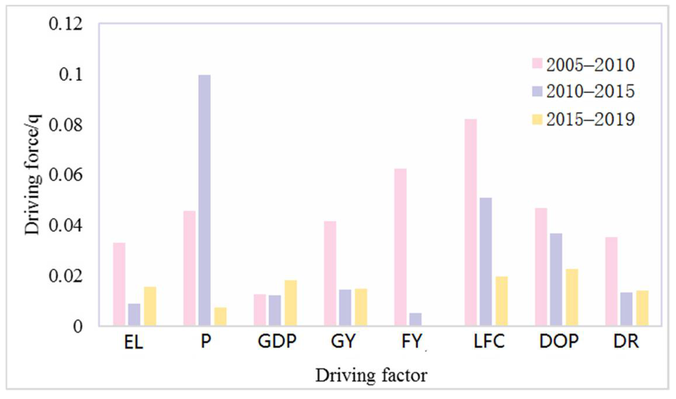
3.3.1. The Factor Detector

As shown in Figure 10, the result of factor detection reflected the driving forces of each driving factor on landscape change. The driving factors of landscape change in the study area at different periods had different intensities. However, factors such as P and LFC had strong driving power throughout the study period. The natural environment of the study area directly determined the pattern of landscape change, to a great extent.

From 2005 to 2010, the driving power of each factor in order on landscape change in Chagan Lake Nature Reserve was LFC > FY > DOP > P > GY > DR > EL > GDP, and the factors with the strongest driving power were LFC and FY. From 2010 to 2015, the driving power of each factor on landscape change in Chagan Lake Nature Reserve was P > LFC > DOP > GDP > GY > DR > FY > EL. The factor with the strongest driving power was P, followed by LFC. From 2015 to 2019, the driving power of each factor on landscape change of Chagan Lake Nature Reserve was DOP > LFC > GDP > EL > GY > DR > P > FY. The driving power q values during this period were all small, indicating that the landscape change of Chagan Lake Nature Reserve from 2015 to 2019 was not dominated by one individual factor.

3.3.2. The Interaction Detector

Interactive detection reflects the difference between the combined effect of multiple factors and the impact of a single factor on landscape change. The interactive impact of two driving factors on landscape change is usually not a simple linear sum. The results of the interactive detection in each period are shown in Figure 11. It could be seen that the interaction detection results between the driving factors in each year all showed two-factor enhancement or nonlinear enhancement, indicating that the driving power of the interaction between the factors on landscape change was enhanced to different degrees compared with single-factor interactions. For example, the q value of P from 2005 to 2010 as a single factor was 0.046, but the q value of interaction between P and other factors was greater than 0.046. Therefore, interactive detection could better explain the reasons for landscape change in the study area.

From the perspective of the whole study period, there were significant differences in the interaction of factors in different years, but the interactions of EL, P, GY, and GY with the other factors all showed strong driving power, indicating that these factors had an impact on landscape change in each period. From 2005 to 2010, the interaction between GY and LFC had the highest intensity (q = 0.226), and the q values of interaction between LFC and EL and P were 0.188 and 0.187. From 2010 to 2015, the q value of the interaction between P and LFC, GY, and DR was the largest, at 0.229, 0.204, and 0.214, respectively. From 2015 to 2019, the q value of the interaction of each factor decreased compared with the previous period, and the interaction force of P and GDP was the largest (q = 0.147), indicating that the landscape change during this period was also affected by other factors besides climate and economic factors.

4. Discussion

4.1. Characteristics of Landscape Pattern Change in the Study Area

From 2005 to 2019, ecological environment management and restoration in the Chagan Lake Nature Reserve have demonstrated remarkable achievements. The water area was increasing, although it is still less than that in 2005. Most of the reduced water area is located in the north and has turned into marshland; the area of bare land has been greatly reduced, and the trend of conversion to grassland and marshland is very obvious. Some grassland has been reclaimed into cultivated land, while the areas of marshland and cultivated land have increased slightly. At the same time, the landscape patches in the study area tended to be regular, while the fragmentation degree of the patches decreased, the connectivity increased, and the landscape heterogeneity increased.

4.2. The Driving Mechanisms

In geospatial regression analysis, if a variable has strong explanatory power in region A, but weak explanatory power in other regions, such a situation where different regions have different properties is considered to be spatial heterogeneity in terms of spatial analysis. Obviously, the regression coefficients of the different drivers of landscape change in the Chagan Lake Nature Reserve have spatial heterogeneity, and the impact of each driving factor on the changes in landscape types in different regions is diverse. For example, the distribution of P in the study area showed a decreasing trend from west to east, while P had a greater impact on the landscape changes in the west, and the spatial distribution of regression coefficients also showed a decreasing trend from west to east. The LFC had a strong impact on the central part of the study area, and its concentration in the central part was significant. The EL had a great impact in the south, which was caused by the higher terrain in the southeast and southwest of the study area.

According to the GWR model, the area where the EL factor had a greater impact is in the south; P had a negative effect on landscape changes in the southeastern and southwestern regions, and the area with the greatest positive impact was in the west; the regression coefficient of GDP was mainly negative in the whole area, and the negative effect was mainly distributed in the north; the area with the greatest negative impact on GY was concentrated in the north; the area with the greatest positive impact on FY changed, from the southeast to the north; the positive impact of LFC was concentrated in the east and south, and the maximum negative influence was located in the southeast; the positive effect of DOP was located in the northern region; the positive impact of DR shifted from the east to the west, and the region with the greatest negative impact was located in the south.

According to factor detection, from 2005 to 2010, LFC had the greatest driving power, which is because the study area is situated in the typical fluorine-rich geochemical environment zone. The dissolution of fluorine-containing minerals is an important source of fluorine in Chagan Lake. At the same time, human activities, such as the expansion of the irrigation area around Chagan Lake, the construction of the river lake connection project in western Jilin, and the exploitation of groundwater have changed the original hydrological and water-quality environment and promoted the enrichment process of fluorine in Chagan Lake, enhancing the driving power of the lake fluoride content on landscape changes. From 2010 to 2015, P had the greatest driving power. This is because the increase in precipitation during this period increased the water area, marshland, grassland, and cultivated land, so the area of bare land was greatly reduced. After 2005, with the weakening of replenishment due to the “Diverting water from Songhua River to Chagan Lake” project, natural precipitation became the main factor affecting the water area of Chagan Lake, which directly affected the marsh area of Chagan Lake Nature Reserve [50]. Therefore, the landscape change of the Chagan Lake Nature Reserve from 2005 to 2015 was mainly affected by natural factors; however, from 2015 to 2019, the landscape change was driven by multiple factors, of which the interaction force of P and GDP was the largest.

The results of interactive detection show that the interaction between various nature and social economy factors has enhanced the strength of the driving factors that affect landscape changes. Such combinations include GY and LFC, P and LFC, and P and GDP.

The results of this paper show that in the past 15 years, natural factors, especially precipitation and lake fluoride content, have had a significant impact on the landscape changes of Chagan Lake Nature Reserve. This result is consistent with most of the other published studies on lakes [51,52]. In contrast, the results show a lesser effect for the factor of the gross domestic product (GDP) compared to the findings of previous studies [53,54]. This is probably due to the economic income of the study area mainly coming from agriculture and tourism. In this study, due to the lack of relevant supporting data, we did not include the total income of tourism, thus causing an underestimation of the impact of social and economic factors.

4.3. Implications for the Lake’s Protection and Management

According to our analysis of the driving mechanisms of the landscape pattern in the Chagan Lake Nature Reserve, factors such as precipitation, lake fluoride content, fishery yield, and grain yield per unit area have a strong driving power on changes in the landscape pattern and present a trend of synergistic enhancement. On the one hand, climate warming and the drought trends in this area have caused significant changes in regional precipitation, and the lake area has shown a tendency to decrease. How to ensure the necessary volume of available water resources in Chagan Lake and the ecological water volume in the surrounding wetlands is, thus, crucial to safeguard the ecological security of the lake. On the other hand, due to the development of land resources around the lake, a large amount of irrigation water from the saline-alkaline paddy fields flowed into Chagan Lake, resulting in a decline in water environment quality and an increase in the fluorine content in the lake water [33]. The reduction and control of pollution sources flowing into the lake and the improvement of water environment quality are urgent problems to be tackled in this area. Therefore, in terms of the governance and management of the areas surrounding the Chagan Lake National Nature Reserve, several actions are urgently needed, including: firstly, the rational allocation of regional water resources, implementing ecological water replenishment, and improving wetland shrinkage and degradation; secondly, the control of regional non-point source pollution, expanding the areas of woodland, grassland and wetland, exploring new techniques suitable for paddy-field planting in saline-alkaline land, encouraging the promotion of using low pollution biotechnology to improve soil, vigorously promoting water-saving irrigation, comprehensively implementing measures to reduce the amount of return water in the irrigation area, and promoting the continuous improvement of the ecological environment of Chagan Lake; thirdly, speeding up the construction of a virtual platform and database for lake monitoring and assessment, building up a digital representation of Chagan Lake, establishing an early-warning system for water level and quality, etc., forming an emergency response mechanism, improving the level of modern management, and reinforcing the scientific decision-making on the management and protection of Chagan Lake.

4.4. Limitations of the Current Research

On the one hand, the Chagan Lake National Nature Reserve has established the Chagan Lake Tourism Economic Development Zone. The annual snow and ice fishing and hunting on the lake in the winter has brought huge economic benefits to the local area. In recent years, in order to meet the needs of tourism, a large number of tourist facilities have been developed in the New Temple area of Chagan Lake, which caused an impact on landscape changes in the study area. However, due to the lack of sufficient data support, such as the figures for the total income from the tourism industry, the number of tourists, etc., it is difficult to quantify the level of landscape change caused by the development of the tourism industry.

On the other hand, this study only sampled and tested fluoride levels in Chagan Lake, while the increase of fluoride concentration in Chagan Lake is related to the dissolution of fluorine-containing minerals and farmland irrigation, both of which require systematic tracking and monitoring, which could be addressed in future research.

5. Conclusions

In this study, remote sensing technology and the geographic information system were used to analyze the landscape types and the landscape index changes of the Chagan Lake Nature Reserve from 2005 to 2019. The main conclusions are as follows:

• In the past 15 years, the main land types in Chagan Lake Nature Reserve were lakes and grasslands, accounting for more than 66% of the total area. The area of lakes increased, while the area of bare land decreased, and the ecological environment has been gradually restored. On the other hand, due to the enhancement of landscape connectivity and the increase of the cultivated land area, a large amount of irrigation has increased the fluorine content in Chagan Lake.
• The temporal and spatial differentiation patterns of the different driving factors of landscape change in Chagan Lake Nature Reserve are diverse. The regression coefficients of P and LFC are large, showing a strong driving force on landscape change. Because the annual precipitation increased year by year during the study period, which is conducive to the growth of vegetation and lake-water storage, this promoted changes in the landscape types, such as grasslands and water areas. At the same time, the study area is located in a typical fluorine-rich geochemical environment. Human activities, such as the expansion of irrigation areas around Chagan Lake, have changed the original hydrological and water-quality environment and promoted the enrichment process of fluorine in Chagan Lake, enhancing the explanatory power of the lake’s fluorine content.
• The driving factors leading to landscape change in Chagan Lake Nature Reserve were different in each period. From 2005 to 2010, the landscape change was mainly affected by LFC, while from 2010 to 2015, it was mainly affected by P. The interaction between P and LFC and other factors showed a strong driving effect, which was an important factor affecting landscape change. From 2015 to 2019, the landscape change in Chagan Lake Nature Reserve was not dominated by individual factors; however, the interaction force of precipitation and the gross domestic product was the largest.

This research will help decision-makers and related stakeholders to make decisions regarding the sustainable development of the Chagan Lake Nature Reserve.

References

1. Kong, F.; Min, X.; Yue, L.; Kong, F.; Wan, C. Wetland landscape pattern change based on GIS and RS: A review. Chin. J. Appl. Ecol. 2013, 24, 941–946. [Google Scholar]
2. Alvarez, D.; Corsi, S.; De Cicco, L.; Villeneuve, D.; Baldwin, A. Identifying Chemicals and Mixtures of Potential Biological Concern Detected in Passive Samplers from Great Lakes Tributaries Using High-Throughput Data and Biological Pathways. Environ. Toxicol. Chem. 2021, 40, 2165–2182. [Google Scholar] [CrossRef] [PubMed]
3. Ducey, M.; Johnson, K.; Belair, E.; Cook, B. The Influence of Human Demography on Land Cover Change in the Great Lakes States, USA. Environ. Manag. 2018, 62, 1089–1107. [Google Scholar] [CrossRef] [PubMed]
4. Liu, L.; Dong, Y.; Kong, M.; Zhou, J.; Zhao, H.; Tang, Z.; Zhang, M.; Wang, Z. Insights into the long-term pollution trends and sources contributions in Lake Taihu, China using multi-statistic analyses models. Chemosphere 2020, 242, 125272. [Google Scholar] [CrossRef]
5. Zhang, T.; Hu, H.; Ma, X.; Zhang, Y. Long-Term Spatiotemporal Variation and Environmental Driving Forces Analyses of Algal Blooms in Taihu Lake Based on Multi-Source Satellite and Land Observations. Water 2020, 12, 1035. [Google Scholar] [CrossRef] [Green Version]
6. Zhang, F.; Yushanjiang, A.; Jing, Y. Assessing and predicting changes of the ecosystem service values based on land use/cover change in Ebinur Lake Wetland National Nature Reserve, Xinjiang, China. Sci. Total Environ. 2019, 656, 1133–1144. [Google Scholar] [CrossRef]
7. Liang, J.; Li, X. Characteristics of temporal-spatial differentiation in landscape pattern vulnerability in Nansihu Lake wetland, China. J. Appl. Ecol. 2018, 29, 626. [Google Scholar]
8. Liu, X.; Zhang, Y.; Dong, G.; Hou, G.; Jiang, M. Landscape pattern changes in the Xingkai Lake Area, northeast China. Int. J. Environ. Res. Public Health 2019, 16, 3820. [Google Scholar] [CrossRef] [Green Version]
9. Zhong, Y.; Lin, A.; Zhou, Z. Evolution of the pattern of spatial expansion of urban land use in the Poyang Lake ecological economic zone. Int. J. Environ. Res. Public Health 2019, 16, 117. [Google Scholar] [CrossRef] [Green Version]
10. Li, L.; Su, F.; Brown, M.; Liu, H.; Wang, T. Assessment of ecosystem service value of the Liaohe estuarine wetland. Appl. Sci. 2018, 8, 2561. [Google Scholar] [CrossRef] [Green Version]
11. Zhou, J.; Wu, J.; Gong, Y. Valuing wetland ecosystem services based on benefit transfer: A meta-analysis of China wetland studies. J. Clean. Prod. 2020, 276, 11. [Google Scholar] [CrossRef]
12. Zhang, L.; Cai, Y.; Jiang, M.; Dai, J.; Guo, X.; Li, W.; Li, Y. The levels of microbial diversity in different water layers of saline Chagan Lake, China. J. Oceanol. Limnol. 2020, 38, 395–407. [Google Scholar] [CrossRef]
13. Haliuc, A.; Buczko, K.; Hutchinson, S.; Acs, E.; Magyari, E.; Korponai, J.; Begy, R.-C.; Vasilache, D.; Zak, M.; Veres, D. Climate and land-use as the main drivers of recent environmental change in a mid altitude mountain lake, Romanian Carpathians. PLoS ONE 2020, 15, e0239209. [Google Scholar] [CrossRef]
14. Chu, L.; Sun, T.; Wang, T.; Li, Z.; Cai, C. Evolution and prediction of landscape pattern and habitat quality based on ca-markov and invest model in Hubei section of Three Gorges reservoir area (TGRA). Sustainability 2018, 10, 3854. [Google Scholar] [CrossRef] [Green Version]
15. Zhang, Y.; Qu, J.; Li, D. Evolution and prediction of coastal wetland landscape pattern: An exploratory study. J. Coastal. Res. 2020, 106, 553–556. [Google Scholar] [CrossRef]
16. Zhao, H.; Zheng, H.; Miao, C.; Shao, T.; Feng, Y. Spatial-temporal pattern and factor diagnoses of agroecosystem health in major grain producing areas of Northeast China: A case study in Jilin Province. Chin. J. Appl. Ecol. 2016, 27, 3290–3298. [Google Scholar]
17. Bie, Q.; Xie, Y. The constraints and driving forces of oasis development in arid region: A case study of the Hexi Corridor in northwest China. Sci. Rep. 2020, 10, 17708. [Google Scholar] [CrossRef]
18. Xiao, M.; Zhang, Q.; Qu, L.; Hussain, H.; Dong, Y.; Zheng, L. Spatiotemporal changes and the driving forces of sloping farmland areas in the Sichuan region. Sustainability 2019, 11, 906. [Google Scholar] [CrossRef] [Green Version]
19. Wang, B.; Li, Y.; Wang, S.; Liu, C.; Zhu, G.; Liu, L. Oasis landscape pattern dynamics in Manas River watershed based on remote sensing and spatial metrics. J. Indian Soc. Remote 2019, 47, 153–163. [Google Scholar] [CrossRef]
20. Liu, C.; Zhang, F.; Johnson, V.; Duan, P.; Kung, H. Spatio-temporal variation of oasis landscape pattern in arid area: Human or natural driving? Ecol. Indic. 2021, 125, 14. [Google Scholar] [CrossRef]
21. Shifaw, E.; Sha, J.; Li, X. Detection of spatiotemporal dynamics of land cover and its drivers using remote sensing and landscape metrics (Pingtan Island, China). Environ. Dev. Sustain. 2020, 22, 1269–1298. [Google Scholar] [CrossRef]
22. Lewandowska-Gwarda, K. Geographically Weighted Regression in the Analysis of Unemployment in Poland. ISPRS Int. J. Geo-Inf. 2018, 7, 17. [Google Scholar] [CrossRef] [Green Version]
23. Fotheringham, A.S.; Oshan, T.M. Geographically weighted regression and multicollinearity: Dispelling the myth. J. Geogr. Syst. 2016, 18, 303–329. [Google Scholar] [CrossRef]
24. Ju, H.; Zhang, Z.; Zuo, L.; Wang, J.; Zhang, S.; Wang, X.; Zhao, X. Driving forces and their interactions of built-up land expansion based on the geographical detector—A case study of Beijing, China. Int. J. Geogr. Inf. Sci. 2016, 30, 2188–2207. [Google Scholar] [CrossRef]
25. Liu, Y.; Cao, X.; Li, T. Identifying Driving Forces of Built-Up Land Expansion Based on the Geographical Detector: A Case Study of Pearl River Delta Urban Agglomeration. Int. J. Environ. Res. Public Health 2020, 17, 1759. [Google Scholar] [CrossRef] [PubMed] [Green Version]
26. Li, J.; Sun, Z. Urban function orientation based on spatiotemporal differences and driving factors of urban construction land. J. Urban Plan. Dev. 2020, 146, 05020011. [Google Scholar] [CrossRef]
27. Meng, X.; Gao, X.; Li, S.; Lei, J. Spatial and temporal characteristics of vegetation NDVI changes and the driving forces in Mongolia during 1982–2015. Remote Sens. 2020, 12, 603. [Google Scholar] [CrossRef] [Green Version]
28. Yan, J.; Chen, J.; Zhang, W.; Ma, F. Determining fluoride distribution and influencing factors in groundwater in Songyuan, Northeast China, using hydrochemical and isotopic methods. J. Geochem. Explor. 2020, 217, 106605. [Google Scholar] [CrossRef]
29. Zhao, W.; Xiao, C.; Chai, Y.; Feng, X.; Liang, X.; Fang, Z. Application of a new improved weighting method, ESO method combined with fuzzy synthetic method, in water quality evaluation of Chagan Lake. Water 2021, 13, 1424. [Google Scholar] [CrossRef]
30. Liu, X.; Zhang, G.; Sun, G.; Wu, Y.; Chen, Y. Assessment of lake water quality and eutrophication risk in an agricultural irrigation area: A case study of the Chagan Lake in northeast China. Water 2019, 11, 2380. [Google Scholar] [CrossRef] [Green Version]
31. Li, S.; Song, K.; Zhao, Y.; Mu, G.; Shao, T.; Ma, J. Absorption characteristics of particulates and CDOM in waters of Chagan Lake and Xinlicheng Reservoir in autumn. Huan Jing Ke Xue 2016, 37, 112–122. [Google Scholar] [PubMed]
32. Liu, X.; Zhang, G.; Zhang, J.; Xu, Y.; Wu, Y.; Wu, Y.; Sun, G.; Chen, Y.; Ma, H. Effects of irrigation discharge on salinity of a large freshwater lake: A case study in Chagan Lake, Northeast China. Water 2020, 12, 2112. [Google Scholar] [CrossRef]
33. Tang, J.; Dai, Y.; Wang, J.; Qu, Y.; Liu, B.; Duan, Y.; Li, Z. Study on environmental factors of fluorine in Chagan Lake catchment, Northeast China. Water 2021, 13, 629. [Google Scholar] [CrossRef]
34. Xu, P.; Bian, J.; Wu, J.; Li, Y.; Ding, F. Distribution of fluoride in groundwater around Chagan Lake and its risk assessment under the influence of human activities. Water Sci. Tech-Water Supply 2020, 20, 2441–2454. [Google Scholar] [CrossRef]
35. Liu, P.; Zheng, C.; Wen, M.; Luo, X.; Wu, Z.; Liu, Y.; Chai, S.; Huang, L. Ecological risk assessment and contamination history of heavy metals in the sediments of Chagan Lake, Northeast China. Water 2021, 13, 894. [Google Scholar] [CrossRef]
36. Wang, F.; Ding, Q.; Zhang, L.; Wang, M.; Wang, Q. Analysis of Land Surface Deformation in Chagan Lake Region Using TCPInSAR. Sustainability 2019, 11, 5090. [Google Scholar] [CrossRef] [Green Version]
37. Yaseen, S.; Shaban, A. Detection of altered water content of AlHammar marshes. In Technologies and Materials for Renewable Energy, Environment and Sustainability; Salame, C.T., Shaban, A., Jabur, A.R., Haider, A.J., Eds.; Elsevier: Amsterdam, The Netherlands, 2020; Volume 2307. [Google Scholar]
38. Hecher, J.; Filippi, A.; Guneralp, I.; Paulus, G. Extracting River Features from Remotely Sensed Data: An Evaluation of Thematic Correctness. In GI_Forum 2013, Creating the GISociety—Conference Proceedings; Wichmann: Berlin, Germany, 2013. [Google Scholar]
39. Zhou, Z.; Li, J. The correlation analysis on the landscape pattern index and hydrological processes in the Yanhe watershed, China. J. Hydrol. 2015, 524, 417–426. [Google Scholar] [CrossRef]
40. Yushanjiang, A.; Zhang, F.; Yu, H.; Kung, H. Quantifying the spatial correlations between landscape pattern and ecosystem service value: A case study in Ebinur Lake Basin, Xinjiang, China. Ecol. Eng. 2018, 113, 94–104. [Google Scholar] [CrossRef]
41. Bell, E.J. Markov analysis of land use change—Application of stochastic processes to remotely sensed data. Socio-Econ. Plan. Sci. 1974, 8, 311–316. [Google Scholar] [CrossRef]
42. Shi, G.; Ye, P.; Ding, L.; Quinones, A.; Li, Y.; Jiang, N. Spatio-temporal patterns of land use and cover change from 1990 to 2010: A case study of Jiangsu province, China. Int. J. Environ. Res. Public Health 2019, 16, 907. [Google Scholar] [CrossRef] [Green Version]
43. Yang, X.; Zheng, X.; Lv, L. A spatiotemporal model of land use change based on ant colony optimization, Markov chain and cellular automata. Ecol. Model. 2012, 233, 11–19. [Google Scholar] [CrossRef]
44. Li, C.; Li, F.; Wu, Z.; Cheng, J. Exploring spatially varying and scale-dependent relationships between soil contamination and landscape patterns using geographically weighted regression. Appl. Geogr. 2017, 82, 101–114. [Google Scholar] [CrossRef]
45. Liu, C.; Wu, X.; Wang, L. Analysis on land ecological security change and affect factors using RS and GWR in the Danjiangkou Reservoir area, China. Appl. Geogr. 2019, 105, 1–14. [Google Scholar] [CrossRef]
46. Yang, C.; Li, R.; Sha, Z. Exploring the dynamics of urban greenness space and their driving factors using geographically weighted regression: A case study in Wuhan metropolis, China. Land 2020, 9, 500. [Google Scholar] [CrossRef]
47. Taillefumier, F.; Piégay, H. Contemporary land use changes in prealpine Mediterranean mountains: A multivariate gis-based approach applied to two municipalities in the Southern French Prealps. Catena 2003, 51, 267–296. [Google Scholar] [CrossRef]
48. Wang, J.; Cai, X.; Chen, F.; Zhang, Z.; Zhang, Y.; Sun, K.; Zhang, T.; Chen, X. Hundred-year spatial trajectory of lake coverage changes in response to human activities over Wuhan. Environ. Res. Lett. 2020, 15, 094022. [Google Scholar] [CrossRef]
49. Cao, F.; Ge, Y.; Wang, J. Optimal discretization for geographical detectors-based risk assessment. Gisci. Remote Sens. 2013, 50, 78–92. [Google Scholar] [CrossRef]
50. Fang, H.; He, Z.; Chen, Q.; Xia, T. Analysis on the temporal and spatial changes of Chagan Lake and its response to precipitation changes during 1985–2018. Sci. Agric. Info. 2020, 32, 64–73. [Google Scholar]
51. Li, Y.; Shi, K.; Zhang, Y.; Zhu, G.; Li, N. Analysis of Water Clarity Decrease in Xin’anjiang Reservoir, China, from 30-Year Landsat TM, ETM+, and OLI Observations. J. Hydrol. 2020, 590, 125476. [Google Scholar] [CrossRef]
52. Karaya, R.N.; Onyango, C.A.; Ogendi, G.M. A community-GIS supported dryland use and cover change assessment: The case of the Njemps flats in Kenya. Cogent Food Agric. 2021, 7, 1872852. [Google Scholar] [CrossRef]
53. Hao, C.; Wanchang, Z.; Huiran, G.; Ning, N. Climate Change and Anthropogenic Impacts on Wetland and Agriculture in the Songnen and Sanjiang Plain, Northeast China. Remote Sens. 2018, 10, 356. [Google Scholar]
54. Balkanlou, K.; Müller, B.; Cord, A.; Panahi, F.; Egli, L. Spatiotemporal dynamics of ecosystem services provision in a degraded ecosystem: A systematic assessment in the Lake Urmia basin, Iran. Sci. Total Environ. 2020, 716, 137100. [Google Scholar] [CrossRef] [PubMed]
Figure 1. Location of the study area (a) China and its provincial borders; (b) the location of the study area in Jilin Province; (c) the image map of the study area in 2010, including the names of the lakes in the study area and the scope of each protected area.
Sustainability 14 05675 g001
Figure 2. The methodological flowchart of the study.
Sustainability 14 05675 g002
Figure 3. Random sampling points (0 means no change in landscape type, 1 means change).
Sustainability 14 05675 g003
Figure 4. Global spatial correlation test results of landscape change in the study area.
Sustainability 14 05675 g004
Figure 5. The types of interaction between the two independent variables and the dependent variable.
Sustainability 14 05675 g005
Figure 6. Landscape type maps of Chagan Lake Nature Reserve from 2005 to 2019. (The core area is the well-preserved natural ecosystem and the concentrated distribution center of rare and endangered animals and plants. Mass passage and tourism activities are prohibited, and scientific research is generally not allowed. The buffer zone allows non-destructive scientific research and specimen collection activities, teaching activities, and, generally, no tourism activities).
Sustainability 14 05675 g006
Figure 7. Changes in area of the landscape types in Chagan Lake Nature Reserve from 2005 to 2019.
Sustainability 14 05675 g007
Figure 8. Spatial distribution of the regression coefficients of natural factors in the GWR model (from top to bottom: EL represents elevation, P represents precipitation, and LFC represents lake fluorine content).
Sustainability 14 05675 g008
Figure 9. Spatial distribution of regression coefficients of the socio-economic factors in the GWR model (from top to bottom: GDP represents the gross domestic product, GY represents grain yield, FY represents fishery yield, DOP represents the distance to oil production, and DR represents the distance to the road).
Sustainability 14 05675 g009
Figure 10. Factor detector of the geographical detector (EL represents elevation, P represents precipitation, GDP represents the gross domestic product, GY represents grain yield, FY represents fishery yield, LFC represents lake fluorine content, DOP represents the distance to oil production, DR represents the distance to the road).
Sustainability 14 05675 g010
Figure 11. Interaction detector images of the geographical detector. (Each color block represents the interaction driving force of the corresponding two driving factors on landscape changes: EL represents elevation, P represents precipitation, GDP represents the gross domestic product, GY represents grain yield, FY represents fishery yield, LFC represents lake fluorine content, DOP represents the distance to oil production, and DR represents the distance to the road).
Sustainability 14 05675 g011