Article

China’s Industrial TFPs at the Prefectural Level and the Law of Their Spatial–Temporal Evolution

School of Economics, Lanzhou University, Lanzhou 730000, China
*
Author to whom correspondence should be addressed.
Sustainability 2023, 15(1), 322; https://doi.org/10.3390/su15010322
Submission received: 8 November 2022 / Revised: 16 December 2022 / Accepted: 21 December 2022 / Published: 25 December 2022

Abstract

:
Calculating China’s industrial total factor productivity (TFP) at the prefectural level comprehensively and accurately is not only an inevitable requirement for China’s industrialization to enter the new development stage of “improving quality and efficiency”, but also a practical need for TFP improvement at the industrial level. Based on the improved Solow residual method with the general nesting spatial model embedded, this paper comprehensively calculated the industrial TFPs of 280 prefectural cities in China from 2003 to 2019, and undertook a detailed analysis of the spatiotemporal evolution law of the calculation results through Dagum’s Gini coefficient and kernel density estimation. Three main conclusions have been drawn in this paper. First, there is an apparent spatial difference among the industrial TFPs of the prefectural cities in China. It is the poorest and has an evident declining trend in northeast China, and best in eastern China, while the development of central and western China is between east and northeast China. Second, the spatial difference level of industrial TFPs of the prefectural cities in China shows a general development trend of firstly falling and then rising. Comparatively speaking, the contribution of intra-group differences is low, while the contribution of inter-group and the intensity of trans-variation are high. Third, the spatiotemporal evolution of China’s industrial TFPs at the prefectural level has the following characteristics: the overall distribution curve moves firstly towards the right and then left, the kernel density at the peak point continuously declines, the distribution ranges are firstly widening and then narrowing, and the tails of the distribution curve are constantly extending. Meanwhile, the distribution figures of the kernel density estimation in different regions show apparent heterogeneity.

1. Introduction

The 20th CPC National Congress held from 16 to 22 October 2022, pointed out that China should focus on the real economy and advance new industrialization to pursue economic growth. Industry is an important part of the real economy and vital for national economic growth. However, the proportion of the added value of the industry in China’s GDP has been decreasing in recent years. In 2021, the ratio was 32.58%, 12.28% lower than in 2002. Under the declining trend of the relative scale of industrial development, it will be an eternal theme for China’s high-quality economic development to fully improve industrial TFPs. The prefectural city is one of the five major administrative levels in China and is located between provinces and counties. Calculating China’s industrial TFPs at the prefectural level accurately, and describing their laws of spatiotemporal evolution systematically, is not only an inevitable requirement for China’s new industrialization but also the practical need for formulating and implementing scientific policies to improve TFPs at the industrial level in China’s prefectural cities.
Industrial TFP is the industrial productivity emphasizing the efficiency after deducting input factors and intermediate inputs from industrial outputs. Recent studies related to the industrial TFP mainly concentrate on the calculation methods. Generally, industrial TFPs are mostly calculated through two dimensions, including frontier and non-frontier. The frontier dimension focuses on the gaps between the actual process in industrial production and the production frontiers. There are two kinds of methods in the frontier dimension, including data envelopment analysis (DEA) and stochastic frontier analysis (SFA). The DEA method is derived from Farrell’s (1957) analysis [1] and developed into a relatively mature paradigm by Charnes et al. (1978) [2] and systematically explained by Tone (2001) [3]. At present, the methods in the DEA family include DEA-CCR, DEA-BBC, DEA-SBM, super efficiency DEA, etc. [4]. The DEA method usually calculates the TFPs combined with some specific indexes, including the Malmquist index [5,6,7], the Luenberger index [8,9], and the ISP index [10]. Under the framework of DEA, the industrial TFP can be decomposed into the rate of changes in industrial resource allocation efficiency and the rate of industrial technological progress. Further, the rate of changes in industrial resource allocation efficiency can be decomposed into the rate of changes in scale efficiency and the rate of changes in factor disposability, and the rate of changes in pure technological efficiency. In contrast, the rate of industrial technological progress can be decomposed into the rate of neutral technology progress and the rate of technological progress with non-neutral inputs [11,12]. The SFA method is derived from the systematic interpretation of Kumbhakar and Lovell (2000) [13,14]. In the SFA analysis, the production function adopts the transcendental logarithmic function, the distribution of the random disturbance term is preset to be the normal distribution, and the distribution of the production inefficiency term is preset to be semi-normal distribution. Under the framework of SFA, the industrial TFP can be decomposed into four parts, including frontier technology progress, relative frontier technology efficiency, resource allocation efficiency, and economies of scale [15]. The above two methods for calculating the industrial TFPs in the frontier dimension have certain defects. The DEA method cannot consider non-input factors and cannot eliminate the correlations between multiple outputs. Meanwhile, the preset function form and distribution form in the SFA method will actually reduce the accuracy of TFP calculation because there is no scientific evidence for the production function or the distributions to be the same as the preset ones.
The non-frontier dimension focuses on calculating industrial TFP through particular algebraic expressions, statistical indexes, or production functions. Nadiri and Prucha (1990) once designed an algebraic expression for the growth rate of TFP, which included three parts: the direct impacts of technological changes, the direct effects of the profit markup of input factors, and the effects of the economies scale [16,17]. Industrial TFP can also be calculated by the difference or ratio of the comprehensive growth rates of the inputs and outputs, and these comprehensive rates are usually obtained by the statistical weighting values of the inputs and the outputs, respectively [18,19,20,21]. The advantage of the methods based on the algebraic expressions and statistical indexes is that they do not need to preset the production function form or the distributions of random variables, and directly use the equations or the indexes to calculate the TFPs. However, the biggest defect of calculating TFP based on the equations or the indexes lies in the imprecision of determining the factor input share. More precisely, there is no special discussion on the shares of capital, labor, and other input factors. Industrial TFPs can also be calculated by the Solow residual method, which is one of the most popular methods in the non-frontier dimension. The core logic for calculating the industrial TFPs by the Solow residual method lies in the ratio between the industrial outputs and the product of each input with its share as exponential. Compared with other non-frontier methods, the advantage of the Solow residual method lies in that the shares of the input factors are included in the calculation process of the TFPs. Basically, the shares of the inputs are equal to the parameters of inputs per capita, which can be estimated from the empirical production function. In the early analysis of the Solow residual method, the empirical production function is usually designed as the Cobb–Douglas production function, and the input factors only include capital and labor, and the relevant parameters are usually estimated by the ordinary least squares under the assumptions of constant returns to scale and technology neutrality [22]. There are many limitations of the Solow residual method in the early analysis. Improvement of these limitations promotes new progress in the Solow residual method and its applications in the field of industrial TFP calculation.
Historically speaking, there are four aspects of expansions in calculating industrial TFP by the Solow residual method. First, extend the Cobb–Douglas function to more general empirical production functions with different formulas of technological progress [23,24]. These more general functions considered the explanatory variables, periods, and their cross terms and usually calculated the growth rate of the TFPs by the difference between the output growth rates and the product of the inputs growth rates and their shares [25,26,27]. Second, refine the substitutional indicators of the explained variables and the explanatory variables in the production function. The refined process of the explained variables is mainly to examine whether choosing the gross values or the added values as the substitutional indicators of the industrial outputs will improve the accuracy of the calculated results of the industrial TFPs. Zhu and Chen (2020) support employing the gross values in the cost and production functions to calculate the industrial TFPs with less heterogeneity [28]. The refined process of the explanatory variables is mainly to select the scientific substitutional indicators of capital and labor and intermediate inputs, while especially some studies decomposed the capital into the investment in construction and installation works and the investment in machinery and equipment [29]. Third, deal with the individual effects differently in the production function. There are three paths for treating these individual effects. The first way is to set the individual effects as fixed and estimate them as in the general panel data modeling. The second way is to estimate the individual effects in the production function using the OP method [30], which decomposes the individual effects into investment and individual investment expectation, takes investment as the proxy variable, and considers the monotonic relationships between outputs and muti-period investment. The third way is to estimate the individual effects using the LP method. The LP method closely approximates the OP method [31]. However, the OP method takes investment as the proxy variable, while the LP method takes intermediate inputs as the proxy variable. Fourth, improve estimation methods of the parameters in the production function. The improved estimation methods mainly include the differential GMM method and consistency estimation considering the survival probability [32,33]. The differential GMM method mitigates the endogeneity of the model by taking the lag term of the explained variable as the instrument variable, while the latter avoids the “survivor bias” by adding the probabilities of the entrance and exit of the enterprises into the model.
Recently, some research pointed out that the industrial TFPs calculated by the Solow residual method and its four expansions were not scientifically accurate because the spillover effects of the explained variable, the explanatory variable, and the random disturbance term are usually ignored in the estimation of the empirical production function [34,35]. Thus, spatial econometrists began to embed spatial econometric models into the calculation methods of TFP. Tientao et al. (2016) used the spatial Durbin model to capture technology spillover and calculate the TFP [34]. Barilla et al. (2020) embedded the general nesting spatial model (GNSM) into the Solow residual method to calculate total factor logistics productivity [35]. However, this kind of embedded analysis is still in the stage of exploration and attempt, and its method logic is not entirely mature. In the analysis of Tientao et al. (2016), the embedded model was not a general formula of the spatial econometric model but the spatial Durbin model (SDM) [34]. In the analysis of Barilla et al. (2020), although the general formula of the spatial econometric model had been taken into account, only four kinds of estimated results from the models of NSM, SAR, SEM, and SAC were reported [35]. Actually, as the general formula of the spatial econometric model, the GNSM could be degraded to seven other spatial econometric models, including NSM, SXL, SAR, SEM, SDM, SDEM, and SAC [36,37]. Thus, there were still four other kinds of estimated results from the potential models that need to be reported. Meanwhile, Barilla’s analysis did not point out the scientific solutions for calculating the TFPs and the shares of the input factors based on the Solow residual method with the GNSM model embedded. After all, the marginal effects of explanatory variables are not directly expressed as their estimated parameters in the spatial econometric analysis. In this paper, GNSM will also be embedded into the Solow residual method to estimate the empirical production function and calculate China’s industrial TFP at the prefectural level. In contrast with the analysis of Barilla et al. (2020) [35], our study will provide scientific solutions for calculating industrial TFPs under the framework of both the Solow residual method and the spatial econometrics, and also choose an optimal model from all the estimated results of the potential models to determine the shares of the input factors. Moreover, the spatiotemporal difference and evolution law of the calculated industrial TFPs of China’s prefectural cities will also be analyzed using Dagum’s Gini coefficient and kernel density estimation. This paper will have three marginal contributions to related research: first, the calculation scale of China’s TFPs will be extended from the provincial level or the enterprise level to the prefectural industrial sector scale; second, the most general formula of the spatial econometric model, GNSM, will be used to improve the Solow residual method, and the scientific solutions for calculating the industrial TFPs and the shares of the input factors under the improved models will also be explained; third, spatial differences and spatiotemporal evolution law of China’s prefectural industrial TFPs are systematically analyzed by the method of Dagum’s Gini coefficient and kernel density estimation.

2. Model Settings and Methods Description

2.1. The Production Function Model for the Industrial Sectors of China’s Prefectural Cities

The GNSM is usually regarded as the most general spatial econometric model because it considers all the spillover effects from the dependent and independent variables and disturbance terms of the spatiotemporal neighbors. We employ the following production function models as shown in Equations (1) and (2) to calculate the industrial TFPs of China’s prefectural cities.
L o g ( Y I P L L I P L ) = α + ρ [ S T W × L o g ( Y I P L L I P L ) ] + β 1 L o g ( K I P L L I P L ) + β 2 L o g ( E I P L L I P L ) + θ 1 [ S T W × L o g ( K I P L L I P L ) ] + θ 2 [ S T W × L o g ( E I P L L I P L ) ] + u i + v t + μ
μ = λ ( S T W × μ ) + ε
In Equation (1), the logarithmic model with variables of inputs and outputs per capita is employed, and the GNSM is also embedded into this logarithmic model. The subscript I P L indicates that the data of the corresponding variables are dealt at the dimension of China’s prefectural industrial sectors. Y indicates the outputs of the industrial sectors of China’s prefectural cities, while K , L , and E separately indicate inputs of capital, labor, and energy of the industrial sectors of China’s prefectural cities. α , β 1 , β 2 , θ 1 , θ 2 are exogenous parameters, u i and v t separately indicate individual fixed effects and period fixed effects, i = 1 , 2 , , N , t = 1 , 2 , , T .
In Equations (1) and (2), S T W is the spatiotemporal weight matrix to reflect the spillover effects among China’s prefectural industrial sectors in the spatial and temporal dimensions. The details of the settings of S T W will be specially discussed later. ρ and λ are spatial correlation parameters. μ and ε are disturbance terms, where ε follows a normal distribution with zero mean and constant variance, and the distribution of μ is decided by Equation (2).

2.2. Settings of Spatiotemporal Weight Matrix

Correct settings of the spatiotemporal weight matrix ( S T W ) are essential for estimating Equations (1) and (2). The S T W , which can accurately reflect the spillover effects in the spatial and temporal dimensions among China’s industrial sectors at the prefectural level, is regarded as the best. However, these spillover effects are usually abstruse, vague, and insubstantial. In this paper, we set the S T W by the Kronecker multiplier of the temporal weight matrix and the spatial weight matrix, as shown in Equations (3)–(7).
S T W = k r o n ( T W , W )
W i j = W i j ( 0 ) j W i j ( 0 ) , W i j ( 0 ) = { 1 d i j 2 , i j 0 , i = j
d i j = r e × arccos [ sin ( ϕ i ξ ) sin ( ϕ j ξ ) + cos ( ϕ i ξ ) cos ( ϕ j ξ ) cos ( φ i ξ φ j ξ ) ]
T W τ υ = T W τ υ ( 0 ) υ T W τ υ ( 0 ) , T W τ υ ( 0 ) = { 0 , τ < υ M o r a n _ I τ M o r a n _ I υ , τ υ
M o r a n _ I τ = N i = 1 N j = 1 N W i j ( η i , τ η ¯ τ ) ( η j , τ η ¯ τ ) ( i = 1 N j = 1 N W i j ) i = 1 N ( η i , τ η ¯ τ ) 2 , η ¯ τ = 1 N i = 1 N η i , τ
In Equation (3), W indicates the spatial weight matrix that reflects the spillover effects among the industrial sectors of the prefectural cities in the same year. T W indicates the temporal weight matrix that reflects the changes in the spillover effects during different periods. S T W is the spatiotemporal weight matrix, and K r o n is the Kronecker multiplier.
The W is constructed as shown in Equations (4) and (5). In Equation (4), W i j ( 0 ) is the element of the W before standardization and is equal to the reciprocal of the square of longitude and latitude distance ( d i j ). The longitude and latitude distance is calculated as in Equation (5), where r e is the earth’s radius and equal to 6378.1 km; i and j are the numbers of the prefectural cities, i j ; φ , ϕ are the longitude and latitude of the prefectural cities; ξ is the empirical constant and equal to π / 180 ; sin ( · ) , cos ( · ) , and arccos ( · ) are the sine function, the cosine function, and the arccosine function. W i j is the row stochastic standardized element of the W , where the standardization method is shown as Equation (4). W i j ( 0 ) is equal to 0 when i = j ; it means the diagonal elements of the W are zeros, and there are no spillover effects when the prefectural cities are the same one.
The T W is constructed in Equations (6) and (7). In Equation (6), T W τ υ ( 0 ) and T W τ υ are the elements of the T W before and after row stochastic standardization. T W τ υ ( 0 ) is calculated by the ratios of the global Moran’s I, as shown in Equation (6). τ , υ are the numbers of periods, M o r a n _ I τ and M o r a n _ I υ are the global Moran’s I at the period of τ and υ calculated based on the W . In Equation (6), when τ is smaller than υ , T W τ υ ( 0 ) is equal to 0; when τ = υ , T W τ υ ( 0 ) is equal to 1; and when τ is bigger than υ , T W τ υ ( 0 ) is equal to the ratio of the global Moran’s I in corresponding years [38]. The global Moran’s I is calculated as shown in Equation (7). In Equation (7), i and j are also the numbers of the prefectural cities; W i j is the element of the spatial weight matrix designed as Equation (4); η i , τ , and η j , τ indicate the values of some economic index reflecting the spillover effects between the prefectural cities i and j at the period of τ ; η ¯ τ is the mean value of this economic index of all the prefectural cities at the period of τ ; N is the total number of the prefectural cities.

2.3. Method of Calculating Industrial TFP of China’s Prefectural Cities: Based on the Improved Solow Residual Method

In the normal analysis of the Solow residual method, the production function is usually preset as Y = A K α L β , where Y is the outputs, and A , K , and L are technology, capital, and labor, α and β are the input share of capital and labor, α + β = 1 , 0 < α < 1 , and 0 < β < 1 . Let y = Y / L and k = K / L , and the TFP and its growth rate will separately be A = y k α ^ , and A A = y y α ^ × k k under the framework of the Solow residual method, where α ^ is the estimated share of the capital input, and the symbol of ‘ indicates the first-order derivative of the corresponding variable. However, if the GNSM is embedded into the Solow residual method, the preset empirical production function model is changed, as in Equations (1) and (2). Thus, the calculation of TFPs and the shares of the input factors will also be changed.
Set Ω 1 = ( I N T ρ × S T W ) 1 , Ω 2 = ( I N T λ × S T W ) 1 , y I P L = Y I P L / L I P L , k I P L = K I P L / L I P L , and e I P L = E I P L / L I P L , and the data generating process (DGP) of the empirical production function model in Equations (1) and (2) can be obtained, as shown in Equation (8).
L o g ( y I P L ) = Ω 1 ( β 1 I N T + θ 1 × S T W ) L o g ( k I P L ) + Ω 1 ( β 2 I N T + θ 2 × S T W ) L o g ( e I P L ) + Ω 1 ( α + u i + v t ) + Ω 1 Ω 2 ε
In Equation (8), I N T is an identity matrix with N × T rows and N × T columns; N and T are, separately, the total number of prefectural cities and years sampled in the model. Taking the natural number as the base, we can obtain the production function under the framework of both the Solow residual method and the spatial econometrics by carrying out power operations for both sides of Equation (8), as shown in Equation (9) [39].
y I P L = A ˜ ( k I P L ) α k ( e I P L ) α e n
In Equation (9), A ˜ = exp [ Ω 1 ( α + u i + v t ) + Ω 1 Ω 2 ε ] ; α k and α e n are the shares of capital and energy, α k = Ω 1 ( β 1 I N T + θ 1 × S T W ) , α e n = Ω 1 ( β 2 I N T + θ 2 × S T W ) ; other expressions are defined the same as in Equations (1) and (2). The production function in Equation (9) is similar to that of the Solow residual method, but the empirical model in Equations (1) and (2) is more accurate because all the spillover effects in industrial production in China’s prefectural cities have been taken into account. We thus define our way to calculate the industrial TFP of China’s prefectural cities as an improved Solow residual method.
By estimating the empirical model in Equations (1) and (2) and its degradation formulas and choosing the optimal estimated model, we can calculate shares of inputs per capita in China’s prefectural industrial sectors. Thus, combined with the shares and the outputs and inputs per capita, the industrial TFPs of China’s prefectural cities can be calculated by the Solow residual method, as shown in Equation (10).
T F P I P L , * ^ = y I P L ( k I P L ) a ^ k , * ( e I P L ) a ^ e n , *
In Equation (10), the definition of y I P L , k I P L , and e I P L is the same as in Equation (9). The symbol of * indicates the optimal model selected from the estimated model of Equations (1) and (2) and its degradation models. T F P I P L , * ^ indicates the calculated industrial TFPs of China’s prefectural cities based on the selected optimal model. a ^ k , * , a ^ e n , * indicate the shares of inputs of capital and energy calculated based on the optimal model selected.
The calculation formulas of the shares of inputs of capital and energy are not the same when the optimal model has a different form, as shown in Table 1. T r a c e ( · ) is the statistic of trace; the hat ( ^ ) above the parameters means the estimated value. GNSM, SDEM, SAC, SDM, SEM, SAR, SXL, and NSM are the eight main spatial econometric models, which are, separately, the abbreviation of the general nesting spatial model, the spatial Durbin error model, the spatial autocorrelation model, the spatial Durbin model, the spatial error model, the spatial autoregressive model, the spatial X-lag model, and the non-spatial model. These eight models have been discussed and used frequently in recent studies after the systematic promotion by Elhorst (2014) [36]. It is worth noting that, because the shares of capital and energy in Equation (9) are matrices with N × T rows and columns, we define the mean value of diagonal elements of these matrices as the final shares of input factors for each optimal model. We did not consider the mean value of all the elements because the input factors in the Solow residual method are not indirect but direct.

2.4. Method of Analyzing the Spatial Differences and Spatiotemporal Evolution Law of China’s Industrial TFPs at the Prefectural Level

2.4.1. Dagum’s Gini Coefficient

Dagum’s Gini coefficient is a vital tool to analyze the spatial difference, and its principal characteristic is to divide the coefficient into three parts: intra-group difference, inter-group difference, and difference in intensity of trans-variation [40]. In this section, the spatial differences of China’s industrial TFPs at the prefectural level will be analyzed based on Dagum’s Gini coefficient, and the temporal evolution law of the spatial differences will also be interpreted through changes in the coefficients in different years, as shown in Equations (11)–(16). In Equation (11), G indicates Dagum’s Gini coefficient; G w , G n b , and G t separately indicates intra-group difference, inter-group difference, and difference in intensity of trans-variation, as shown in Equation (12).
G = G w + G n b + G t
G w = j = 1 k G j j P j S j , G n b = j = 1 k h j G j h ( P j S h + P h S j ) D j h , G t = j = 1 k h j G j h ( P j S h + P h S j ) ( 1 D j h )
G j j = i = 1 n j l = 1 n j | T F P I P L , j i ^ T F P I P L , j l ^ | 2 n j 2 T F P I P L , j ^ ¯ , G j h = i = 1 n j r = 1 n h | T F P I P L , j i ^ T F P I P L , h r ^ | n j n h ( T F P I P L , j ^ ¯ + T F P I P L , h ^ ¯ )
P j = N j N , S j = N j T F P I P L , j ^ ¯ N T F P I P L ^ ¯ , S h = N h T F P I P L , h ^ ¯ N T F P I P L ^ , D j h = d j h p j h d j h + p j h
d j h = 0 d F j ( T F P I P L , j i ^ ) 0 T F P I P L , j i ^ ( T F P I P L , j i ^ T F P I P L , h r ^ ) d F h ( T F P I P L , h r ^ )
p j h = 0 d F h ( T F P I P L , j i ^ ) 0 T F P I P L , j i ^ ( T F P I P L , j i ^ T F P I P L , h r ^ ) d F j ( T F P I P L , h r ^ )
In Equation (12), G j j is the intra-group Gini coefficient of industrial TFPs of China’s prefectural cities, while G j h is the inter-group Gini coefficient. The definition of G j j and G j h is shown as in Equation (13), where j and h are different spatial groups divided. In Equation (12), P j is the ratio of prefectural cities of the spatial group j in all the prefectural cities; S j and S h indicate the proportions of the sum of the industrial TFPs in spatial groups j and h in the sum of the industrial TFPs of all the prefectural cities; T F P I P L , j ^ ¯ and T F P I P L , h ^ ¯ indicate the mean values of industrial TFPs of prefectural cities in the spatial group j and h ; T F P I P L ^ ¯ indicates the mean value of industrial TFPs of all the prefectural cities; N j and N h are the numbers of prefectural cities in the spatial group j and h ; D j h indicates the relative influence power between spatial group j and h . The definitions P j , S j , S h , D j h are shown in Equation (14). d j h indicates the sum of influences of both spatial group j and h , as shown in Equation (15), while p j h indicates the first moment of trans-variation between spatial group j and h , as shown in Equation (16).

2.4.2. Kernel Density Estimation

Kernel density estimation (KDE) is another important method for analyzing the laws of spatiotemporal evolution [41,42]. Generally, KDE explains the characteristic of the empirical distribution of a variable by particular kernel function and bandwidth. It can describe the spatiotemporal evolution law by the changes in the empirical distributions in different periods. There are many kernel functions, such as Gaussian and bi-square functions, etc., and various bandwidth settings, such as fixed or adaptive, etc.
Suppose the industrial TFP of China’s prefectural cities is a random variable with independent and identical distribution, and the estimated industrial TFPs of China’s prefectural cities based on the selected optimal spatial model are the samples of the random variable. Moreover, suppose f ( · ) and F ( · ) are separately the probability density function and cumulative probability distribution function of the variable of the industrial TFP, where F ( T F P 0 ) = P r o b ( T F P < T F P 0 ) , and T F P 0 is the value of one of the industrial TFPs. Thus, the KDE value of the industrial TFPs of China’s prefectural cities can be defined as Equation (17).
f ( T F P τ ^ ¯ ) = 1 N × h h i = 1 N K ( T F P i , τ ^ T F P τ ^ ¯ h h )
In Equation (17), K ( · ) is the kernel function and h h is the bandwidth. T F P τ ^ ¯ is the mean value of the estimated industrial TFPs of China’s prefectural cities at the period of τ , which can be calculated by the mean value of T F P ^ i , τ in a particular year. Furthermore, we adopt the Gaussian kernel function and select the optimal bandwidth by the principle of minimum average integral error in this paper.

3. Data Processing of Related Variables and Their Description Statistics

As shown in Equations (1) and (2), the industrial growth in China’s prefectural cities is mainly decided by the inputs of factors of capital, labor, and energy of the industry sectors. We will take the gross value of industrial outputs in China’s prefectural cities as the output index in this paper, and take industrial capital stock, industrial total employed persons, and industrial electricity consumption as the inputs of factors of capital, labor, and energy of the industry sectors in China’s prefectural cities. The period adopted in our research is 2003–2019. The main reason is that China formally implemented the new industrialization strategy in 2003, which has new requirements for higher production efficiency of the industrial sectors; meanwhile, for the sake of comparative completeness of the data, we limit the deadline of our research cycle to 2019.
The prefectural cities adopted in our study include 265 prefectural cities and 15 sub-provincial cities. The 265 prefectural cities include all the prefectural cities in China excluding Danzhou and Sansha in Hainan, Chaohu in Anhui, Laiwu in Shandong, Bijie and Tongren in Guizhou, Haidong in Qinghai, Turpan and Hami in Xinjiang, and Xigaze, Changdu, Linzhi, Shannan and Naqu in Tibet, because they adjusted the administrative level from lower level during 2003–2019. The 15 sub-provincial cities include Guangzhou, Wuhan, Harbin, Shenyang, Chengdu, Nanjing, Xi’an, Changchun, Jinan, Hangzhou, Dalian, Qingdao, Shenzhen, Xiamen, and Ningbo. It is worth pointing out that the four municipalities of Beijing, Shanghai, Tianjin, and Chongqing, and the two unique administrative regions of Hong Kong and Macao, are excluded from our research because their scale of industrial growth is different from the 280 cities employed in our study.
We collected related data firstly from the EPS statistical database, China economic and social development statistical database, DRCnet statistical database, China urban statistical yearbook, China regional statistical yearbook, and China statistical yearbook, etc., and then processed the data as follows: First, the total industrial output value above designated size is used to replace the gross value of industrial outputs at the prefectural level. Second, industrial capital stock in China’s prefectural cities is calculated by the perpetual inventory method, as shown in Equation (18).
K t , I P L = K t 1 , I P L × ( 1 η I P L ) + ( I t , I P L / P t , I P L ) × 100
In Equation (18), K t , I P L indicates the actual industrial capital stock at the prefectural level in the year t , K t 1 , I P L indicates the actual industrial capital stock at the prefectural level in the previous year t 1 , η I P L is the depreciation rate, I t , I P L indicates the added fixed assets in the prefectural industrial sectors in the year t , and P t , I P L is the fixed-asset investment prices index. Third, the related data are adjusted to their actual values, taking 1990 as the base period. More details of the data processing can be found in our related study [42]. Then, the descriptive statistical properties of the relevant data can be obtained by summarizing the data of the inputs and outputs in industrial sectors in China’s 280 prefectural cities during 2003–2019 and reshaping them in the way of cities first and then period, as shown in Table 2.

4. The Calculation Results of China’s Industrial TFPs at the Prefectural Level and the Analysis of the Law of Their Spatiotemporal Evolutions

4.1. The Spatial and Temporal Weight Matrices

In the calculation process of industrial TFPs with the GNSM embedded, the spatiotemporal weight matrix needs to be exogenous. There are many types of exogenous spatiotemporal weight matrices, such as the spatiotemporal weight matrix with the elements equal to the reciprocal of Euclidean distances in three-dimensional space, the spatiotemporal weight matrix with the elements equal to ones when the distances in the spatial and temporal dimensions are less than a specific value, the Kronecker multiplier of the identity matrix and the spatial weight matrix, and the Kronecker multiplier of the lower triangular matrix with all the element equal to ones and the spatial weight matrix, etc. However, these types of exogenous spatiotemporal weight matrices cannot capture the real spillover effects and their changes among different periods accurately because of their subjective settings.
In this paper, we introduce a new spatiotemporal weight matrix to more accurately capture the real spillover effects among the prefectural cities and their changes during the sampling periods, as shown in Equations (3)–(7). According to Equations (4) and (5), the spatial weight matrix reflecting the spillover effects of China’s 280 prefecture cities can be determined as shown in Figure 1a. On this basis, we can determine the temporal weight matrix by calculating the global Moran’s I in each year and the ratios between any two years, as shown in Figure 1b. Subsequently, the spatiotemporal weight matrix can be determined by the Kronecker multiplier of the temporal weight matrix and the spatial weight matrix, as shown in Figure 1c.
It is worth noting that the global Moran’s I in the year τ ( M o r a n _ I τ ) can be calculated according to Equation (7), where we define η as the values of some economic index in the previous analysis. This economic index should reflect the real spillover effects among the prefectural cities and their changes during the sampling periods, and also be independent of the explained variable and the explanatory variables for eliminating the endogeneity. We take the estimated residuals ( ^ ) of the model of Equation (19) as the alternative value of the economic index. In Equation (19), ξ 0 , ξ 1 , ξ 2 are exogenous parameters, and ^ is the random disturbance term. Other variables and symbols are defined the same as in Equation (1).
L o g ( Y I P L / L I P L ) = ξ 0 + ξ 1 L o g ( K I P L / L I P L ) + ξ 2 L o g ( E I P L / L I P L ) +

4.2. Selection of the Optimal Estimated Model and Calculation of China’s Industrial TFPs at the Prefectural Level

The selection of the optimal model of the estimated production function is a milestone step for calculating China’s industrial TFPs at the prefectural level. Basically, in spatial econometric models, we consider first whether the model has spatial effects or not and which types of spatial effects should be considered in the model, and then investigate the individual or period fixed effects or random effects. Therefore, based on the spatiotemporal weight matrix in Figure 1c and the data of the variables of inputs and outputs, we first estimated eight spatial econometric models without individual fixed effects and period fixed effects and random effects, as shown in Table 3. The eight models include the model in Equations (1) and (2) and their seven degradation models.
In Table 3, the goodness of fit of the models of SAR, SDM, and SEM is negative, the estimated parameter of the composed variable ( S T W × L o g ( K / L ) ) is not significant in the model of SDEM, and the estimated spatial autoregressive coefficient of the model of SAC is negative and inconsistent with the calculated value of the global Moran’s I. Therefore, the optimal model cannot be these five models. Meanwhile, although the estimated parameters are significant and the statistical properties of the GNSM are also good, the GNSM cannot be the optimal model because the former five models that are less general are not the optimal model. Thereby, the optimal model will be one of the two models between SXL and NSM.
Comparing the two candidates, the goodness of fit and log-likelihood of the SXL are more significant than those of the NSM, and the estimated variance of the random disturbance term of the SXL is smaller than that of the NSM. Thus, the SXL might be the optimal model for the empirical production function of China’s industrial sectors at the prefectural level. Further investigation of the individual or period fixed effects or random effects will help to select the optimal model between the two candidates. We list the estimated results of the two candidate models with different fixed effects in Table 4 below. We do not consider the models of the SXL and NSM with random effects because almost all the spatial units at the prefectural level are included in our analysis [43]. From Table 4, the SXL is better than the NSM because of the following three points: first, the significances of the estimated parameters in the SXL of three kinds of fixed effects are better than those of the NSM; second, the goodness of fit and the log-likelihood of the SXL with three different fixed effects are more significant than those of the NSM; third, the estimated variances of the disturbance terms of the SXL model with other fixed effects are lower than those of the NSM.
We discuss the specific form of the fixed effects of the SXL further by LR tests after choosing the SXL as the potential optimal model. We compare the two models of the SXL with individual fixed effects and without any fixed effects through the LR test with the null hypothesis H 0 , 1 : μ 1 = μ 2 = = μ 280 , where the LR Statistic, equal to minus twice the differences between the log-likelihood values of the two models, obeys the chi-square distribution with 280 degrees of freedom. We also compare the two models of the SXL with period fixed effects and without any fixed effects through the LR test with the null hypothesis H 0 , 2 : ν 1 = ν 2 = = ν 17 , where the LR statistic obeys the chi-square distribution with 17 degrees of freedom. From comparing the two LR statistics above (6631.8 and 868.8, respectively) and their critical values, the SXL with individual fixed effects or period fixed effects is better than that without any fixed effects. On this basis, further discussion should be made among the models of the SXL with three different fixed effects. We also use LR tests to select the SXL with appropriate fixed effects with the null hypotheses of H 0 , 3 : ν 1 = ν 2 = = ν 17 and H 0 , 4 : μ 1 = μ 2 = = μ 280 . We can determine that the SXL with both individual and period fixed effects is better than the model with either individual or period fixed effects because the LR statistic under the null hypothesis of H 0 , 3 and H 0 , 4 (960.85 and 6723.9, respectively) are both bigger than the critical values. The estimated results of the selected optimal model are listed in the seventh column of Table 4.
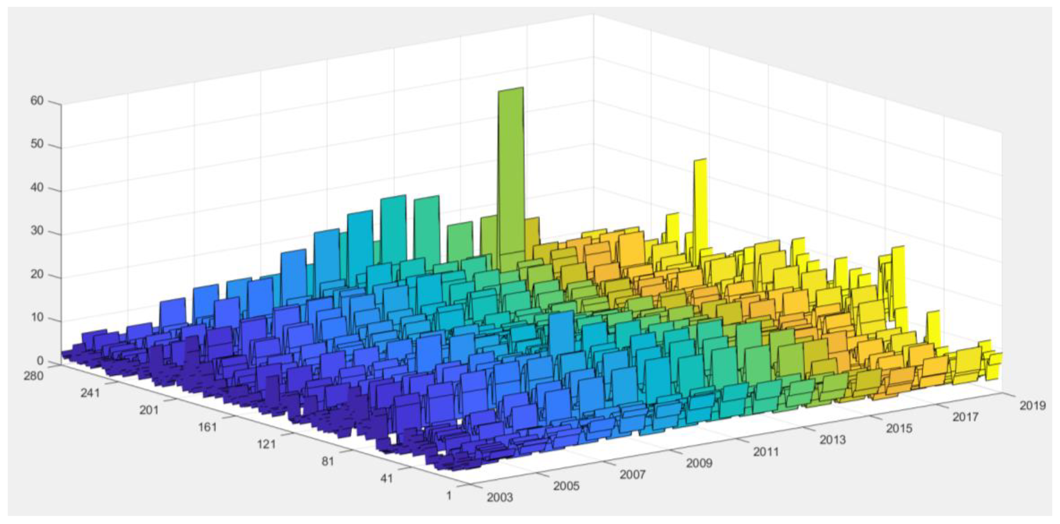
As analyzed above, the selected optimal model is the SXL with both individual and period fixed effects. It is a degradation form of Equations (1) and (2) with the conditions of ρ = 0 and λ = 0 . In the selected optimal model, the spatial spillover effects of the explained variables and random disturbance terms are not obvious in the industrial production process in China’s prefectural cities. These spatial spillover effects are mainly reflected in the explanatory variables. Specifically, the elasticity of capital per capita and energy consumption per capita in the spatial adjacent regions to the outputs per capita in prefectural industrial sectors is 0.519 and 0.4655, respectively. These results are consistent with the positive global Moran’s I. It is worth noting that, these values of elasticity have no significant economic meanings because we usually did not use them to calculate the industrial TFPs and the shares of input factors directly. Moreover, from the estimated result of the selected optimal model, the elasticity of local capital per capita and local energy consumption per capita to the outputs per capita in prefectural industrial sectors is 0.5649 and 0.1202, respectively. These two values of elasticity also have no special economic significance because we cannot treat these values as the shares of the corresponding input factors directly. Although there is no special economic significance for the above four elasticity values, we are supposed to estimate all the models listed in Table 3 and Table 4 and select the best model to calculate the shares of inputs and the industrial TFPs as stated in Table 1. Based on the estimated results of the optimal model, combined with Table 1, shares of inputs of capital and energy in China’s prefectural industrial sectors can be determined, where the share of capital is 0.5649 while the share of energy is 0.1201. Under the assumption of Hicks’ neutral technological progress and constant returns to scale, the input share of the labor factor in China’s prefectural industrial sectors will be 0.3150. Thereafter, according to Equation (10), the industrial TFPs of China’s 280 prefectural cities during 2003–2019 can be calculated, as shown in Figure 2 below.

4.3. The Spatiotemporal Evolution Law of China’s Industrial TFPs at the Prefectural Level

Based on the methods of the Dagum’s Gini coefficient and the kernel density estimation explained in Equations (11)–(17) and the basic mean value analysis, the spatiotemporal evolution characteristics of China’s industrial TFPs at the prefectural level can be analyzed as follows.
(1)
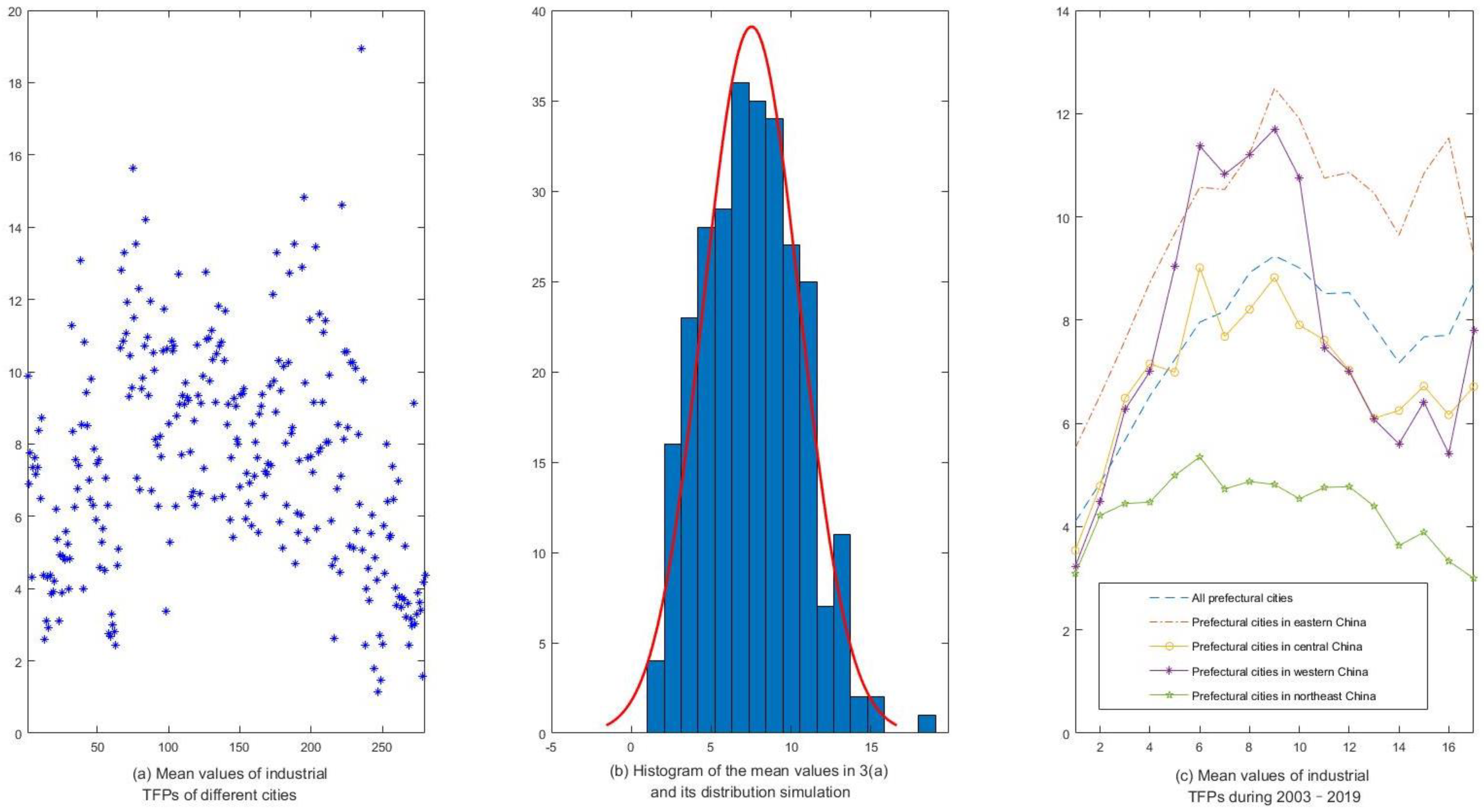
There is an apparent spatial difference among China’s industrial TFPs at the prefectural level; it is best in eastern China and poorest in northeast China. Figure 3 below shows the mean value of the industrial TFPs at the prefectural level by region or period, where subgraph (a) shows the average industrial TFPs of the 280 prefectural cities, subgraph (b) shows the histogram of the average industrial TFPs in subgraph (a) and its simulation of normal distribution, and the subgraph (c) shows the average industrial TFPs in the year from 2003 to 2019. From Figure 3a, there is a significant spatial difference in the mean value of China’s industrial TFPs at the prefectural level, and its range is about 1~19. From Figure 3b, the mean value of China’s industrial TFPs at the prefectural level has an inevitable concentration trend. There are 156 cities with an average industrial TFP between 5 and 10, accounting for 55.71% of all the prefectural cities. From Figure 3c, during 2003–2019, the mean values of industrial TFPs of the prefectural cities in eastern China are higher than the mean values of the 280 prefectural cities, the mean values of industrial TFPs of the prefectural cities in northeast China are lower than the mean values of all the prefectural cities, and the mean values of the industrial TFPs of the prefectural cities in central and western China fluctuate considerably. From the perspective of development trends, the industrial TFPs of China’s prefectural cities show a trend of first rising, then declining, and then slowly recovering, where the recovery and development trends are apparent in central and western China recently, and there is still a downward trend in eastern and northeastern China in recent years.
(2)
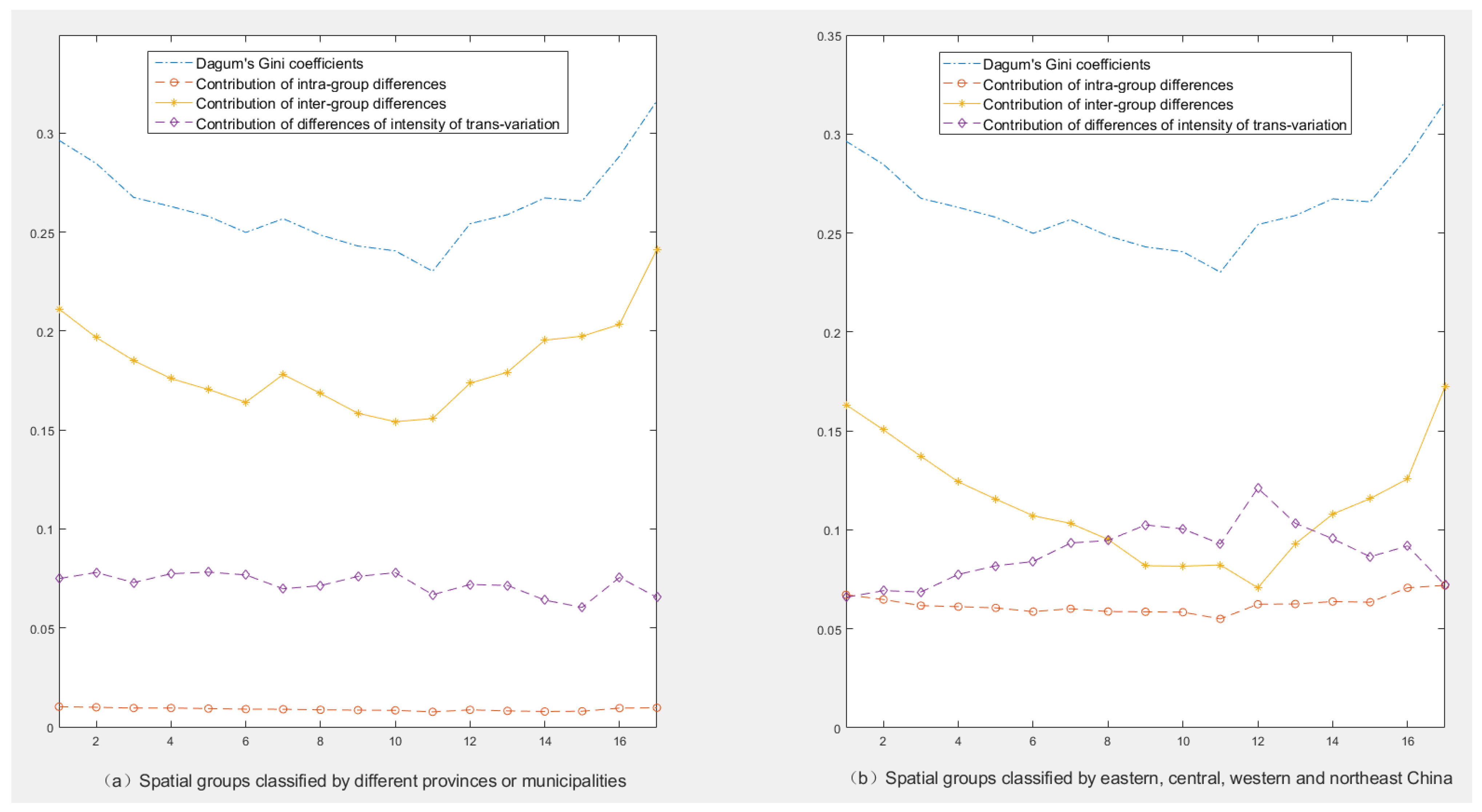
The spatial difference level of China’s industrial TFPs at the prefectural level presents a general development trend of firstly decreasing and then rising, with a relatively lower contribution of intra-group differences, while the somewhat higher contribution of both the inter-group differences and the intensity of trans-variation differences. Figure 4 shows the Dagum’s Gini coefficients of China’s industrial TFPs at the prefectural level and their contributions originating from three parts, including the intra-group difference, the inter-group difference, and the difference in intensity of trans-variation. It is worth noting that the spatial groups in Figure 4a are classified by the prefectural cities belonging to different provinces or municipalities, while the spatial groups in Figure 4b are classified by the prefectural cities belonging to eastern, central, western, or northeast China. In Figure 4a, the overall Gini coefficient and the contribution part from the inter-group difference show U-shaped trends of firstly declining and then rising. The contribution part from the inter-group difference is higher than the contribution part separately from the intra-group difference and the difference in intensity of trans-variation. Moreover, the changes in the contributions from the intra-group difference and the difference in intensity of trans-variation are relatively gentle. In Figure 4b, the overall Gini coefficient and the contribution part from the inter-group difference also show the same trends as in Figure 4a. In contrast, the contributions from the inter-group difference and the difference in intensity of trans-variation are higher and fluctuate more than the contribution from the third part. Comparing Figure 4a with Figure 4b, under the different classifications of the spatial groups, the overall Gini coefficient is the same, and the contribution of the difference in intensity of trans-variation is also almost the same. However, the contribution from the intra-group differences is higher under the spatial groups classified according to eastern, central, western, and northeast China. In comparison, the contribution from the inter-group differences is higher on the condition of the spatial groups divided by the provincial administrative regions.
(3)
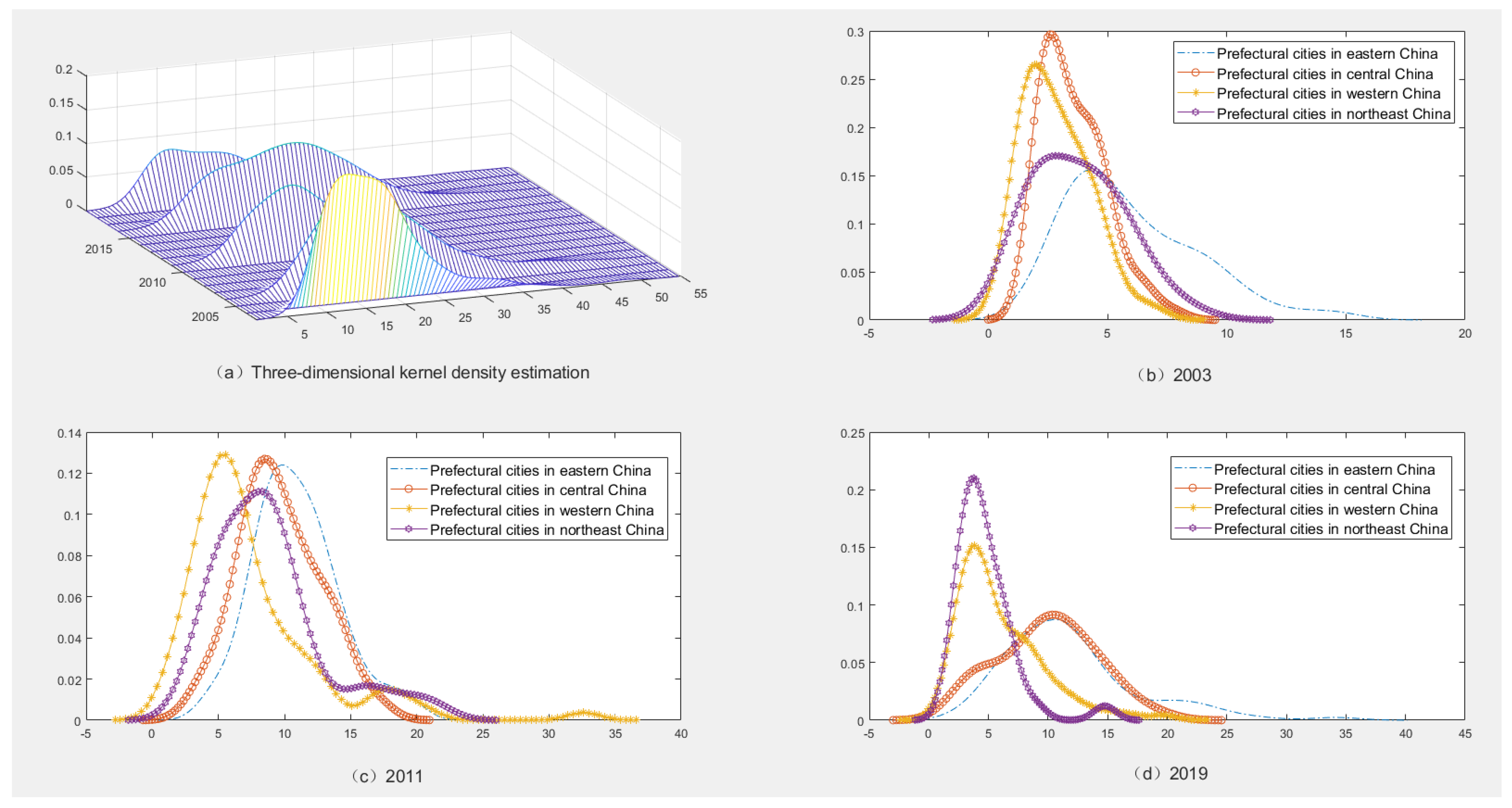
The spatiotemporal evolution of China’s industrial TFP at the prefectural level has the following characteristics: the overall distribution curve moves towards firstly right and then towards left, the kernel density at the peak point continuously declines, and the distribution ranges are first widening and then narrowing. Figure 5a below shows the three-dimensional kernel density estimation of China’s industrial TFPs at the prefectural level in 2003, 2006, 2011, 2016, and 2019. From Figure 5a, compared with 2003, the overall distribution curve of the kernel density estimation shifts to the right in 2006, while the kernel density at the peak decreases, and the distribution range widens; compared with 2006, the distribution curve continued to shift to the right in 2011, the kernel density at the peak continues to decrease, and the distribution range continues to widen; compared with 2011, the distribution curve began to shift to the left in 2016, and the kernel density at the peak increases slightly, but the distribution range narrows; compared with 2016, the distribution curve shifts to the right slightly in 2019, the kernel density at the peak flatters and decreases, the distribution range widens. The tail of the distribution curve on the right side obviously extends.
(4)
There are also obvious spatial heterogeneities in the kernel density estimation of China’s industrial TFPs at the prefectural level. Figure 5b–d below separately show the two-dimensional kernel density estimation of the industrial TFPs of the prefectural cities belonging to eastern, central, western, and northeast China in 2003, 2011, and 2019. In Figure 5b, compared with the prefectural cities in central China, the distribution curve of the kernel density estimation of the industrial TFPs of the prefectural cities in eastern China in 2003 moves towards the right, the kernel density at the peak obviously decreases, the distribution range widens, and the tail of the distribution curve on the right side obviously extends; compared with the prefectural cities in central China, the distribution curve of the western prefectural cities in 2003 moves towards the left, the kernel density at the peak is also decreasing, the distribution range almost stays the same; compared with the western prefectural cities, the distribution curve of the northeast prefectural cities in 2003 moves towards the right slightly, the kernel density at the peak decreases while the distribution range obviously widens. The spatial heterogeneities of the kernel density estimation in 2011 and 2019 can also be analyzed in the same way as in 2003. In detail, we list the relative changes in the distribution curve, the kernel density at the peak point, the distribution range, and the tails of the distribution curve in the four regions, as shown in Table 5.

5. Conclusions and Further Research Directions

In the former analysis, we calculated the industrial TFPs of China’s 280 prefectural cities during 2003–2019 using the improved Solow residual method with the GNSM embedded; we also analyzed the spatiotemporal evolution law of the industrial TFPs with the mean value analysis and the Dagum’s Gini coefficient and the kernel density estimation. Many important conclusions can be drawn as follows:
(1)
The optimal model of the estimated production functions of the industrial sectors in China’s prefectural cities is the SXL with both the individual fixed effects and the period fixed effects. From this optimal model, China’s industrial TFPs at the prefectural level can be calculated scientifically. From the calculation results, there are apparent spatial heterogeneities in these industrial TFPs, where the industrial TFPs of the prefectural cities in eastern China are higher, and those in northeast China are lower, while the industrial TFPs of the prefectural cities in central and western China fluctuate considerably.
(2)
The level of spatial differences of China’s industrial TFPs at the prefectural level shows an overall trend of first decreasing and then rising. Comparatively, the decomposed contribution of the general Gini coefficients from the intra-group differences is lower, and the contributions from the inter-group differences and the differences in the intensity of trans-variation are higher.
(3)
The spatiotemporal evolution of China’s industrial TFPs at the prefectural level has the following characteristics: first, the overall distribution curve moves firstly towards the right and then left; second, the kernel density at the peak point continuously declines; third, the distribution ranges are first widening and then narrowing; fourth, the tails of the distribution curve are constantly extending. Meanwhile, the distribution figures of the kernel density estimation in different regions show apparent heterogeneity.
In our study, three efforts have been made: first, we extend the research of Barilla et al. (2020) [35], introduce an improved Solow residual method with the GNSM embedded, and provide the general solution for calculating the industrial TFPs and the shares of inputs in industrial sectors. Second, we calculate industrial TFPs at the level of China’s prefectural cities based on the optimal production function model chosen from the eight kinds of estimated models, including the GNSM and its degradation forms. These TFPs are traditionally calculated at the macro level of provinces or the micro level of enterprises, and the empirical production function employed to calculate these TFPs is usually the C-D function without spatial spillover taken into account. Third, we use the method of Dagum’s Gini coefficient and kernel density estimation to analyze the spatial–temporal evolution law of the industrial TFPs in China’s prefectural cities. Although our efforts will contribute to the new development of related research to some extent, there are still some works that need to be conducted in the future, including embedding spatial econometrics into the TFP calculation methods in the frontier dimension, such as SFA, and comparing the calculation results from the improved methods in both the frontier and non-frontier dimensions, and decomposing the main influencing factors for the industrial TFPs in China’s prefectural cities. The above three issues need future concentration.

6. Policy Suggestions

Based on the main conclusions above, we suggest formulating and implementing the following policies to improve the industrial TFPs of China’s prefectural cities and constantly reduce the development gap of the industrial TFPs among different prefectural cities.
(1)
Further improve the resource allocation efficiency of China’s industrial sectors at the prefectural level. From Equation (10), the industrial TFPs in China’s prefectural cities are determined by three parts: the industrial outputs per capita, the inputs of capital per capita and energy per capita in the industrial sectors, and the shares of capital and energy. Moreover, higher outputs and lower inputs and their shares will lead to higher industrial TFPs. Therefore, improving the allocation efficiency of capital, labor, and energy will be a necessary means to improve the industrial TFPs in China’s prefectural cities. Here, we propose three suggestions for improving the allocation efficiency of the three main input factors. First, the capital should be guided actively to invest in regions with lower industrial TFPs with more favorable tax subsidies, land concessions, etc. Second, the establishment of colleges and vocational schools should be actively promoted in the prefectural cities to cultivate high-level skilled talents and workers needed for industrial development. Third, the construction of industrial energy storage bases and related equipment (such as photovoltaic power generation, etc.) should be further strengthened through special subsidies to reduce the cost of industrial electricity consumption.
(2)
Further promote industrial and technological innovation to improve the industrial TFPs of China’s prefectural cities comprehensively. Generally, industrial innovation and technological innovation are vital paths to the growth of industrial outputs. These two kinds of innovations can also change the structure of industrial input factors and then promote the development of the industrial sectors in China’s prefectural cities. As a matter of fact, the improvement of industrial TFPs itself is an important manifestation of industrial innovation and technological innovation, and also an inevitable result of these innovative developments. Therefore, we suggest promoting industrial innovation and technological innovation from the following three aspects: First, strengthen the supply side structural reform and find the scientific mode and path to promote the high-quality development of the industrial sectors at the prefectural level. Second, accelerate the application of new concepts, new business types, and new scenes (such as intelligent digital manufacturing, “Internet plus”, artificial intelligence, and the meta-universe, etc.) in the industrial sectors to cultivate new drivers of industrial development. Third, promote new technologies to be the inexhaustible driving force for the improvement of China’s industrial TFPs at the prefectural level by more applications of new generation technologies (such as industrial robots, cloud computing, and the internet of things) in the industrial sectors.
(3)
Promote the coordinated development of the industrial TFPs of China’s prefectural cities through effective regional coordination among industries of different cities. The biggest obstacle to the overall improvement of the industrial TFPs in China’s prefectural cities lies in their imbalance among different regions. Specifically, there are big gaps between the development levels of the industrial TFPs in the prefectural cities between eastern and northeast China. This problem requires special attention. We hope that the coordinated development of the industries among different regions will help to promote the overall improvement of the industrial TFPs in China’s prefectural cities. Thus, we provide three suggestions to improve the TFPs from the perspective of industrial-coordinated development. First, promote the efficient transfer of industries from eastern and central China to the vast western and northeast China, and enhance the environmental protection examination in the transfer of the industries comprehensively considering the resource endowment and development conditions of the cities where the industries are transferred. Second, strengthen the co-construction and sharing of industrial data and resources. Moreover, build a new integrated development pattern of industrial services by constructing regional industrial service platforms. Third, promote the development of the industrial sectors collaboratively by further strengthening the integration of resources of the industrial sectors in the prefectural cities, primarily through the integration of the platforms of the enclave industrial zones and adjacent industrial zones, etc.

Author Contributions

Conceptualization, W.W., Q.F., A.G.; methodology, Q.F.; software, Q.F.; validation, W.W., Q.F., A.G.; formal analysis, W.W., Q.F.; investigation, W.W.; resources, Q.F.; data curation, Q.F.; writing—original draft preparation, W.W., Q.F.; writing—review and editing, Q.F.; visualization, Q.F.; supervision, A.G.; project administration, W.W., Q.F., A.G.; funding acquisition, A.G. All authors have read and agreed to the published version of the manuscript.

Funding

This work was partly sponsored by the National Social Science Foundation of China (20XJL008).

Institutional Review Board Statement

Not applicable.

Informed Consent Statement

Not applicable.

Data Availability Statement

The data presented in this study are available upon request from the corresponding author.

Conflicts of Interest

The authors declare no conflict of interest.

References

  1. Farrell, M.J. The measurement of productive efficiency. J. R. Stat. Soc. A Stat. 1957, 120, 253–290. [Google Scholar] [CrossRef]
  2. Charnes, A.; Cooper, W.W.; Rhodes, E. Measuring the efficiency of decision-making units. Eur. J. Oper. Res. 1978, 2, 429–444. [Google Scholar] [CrossRef]
  3. Tone, K. A slacks-based measure of efficiency in data envelopment analysis. Eur. J. Oper. Res. 2001, 130, 498–509. [Google Scholar] [CrossRef] [Green Version]
  4. Yang, X.; Jia, Z.; Yang, Z. How does technological progress impact transportation green total factor productivity: A spatial econometric perspective. Energy Rep. 2021, 7, 3935–3950. [Google Scholar] [CrossRef]
  5. Malmquist, S. Index numbers and indifference surfaces. Trabajos de Estadistica 1953, 4, 209–242. [Google Scholar] [CrossRef]
  6. Caves, D.W.; Christensen, L.R.; Diewert, W.E. The economic theory of index numbers and the measurement of input, output, and productivity. Econometrica 1982, 50, 1393–1414. [Google Scholar] [CrossRef]
  7. Shen, N.; Liao, H.; Deng, R.; Wang, Q. Different types of environmental regulations and the heterogeneous influence on the environmental total factor productivity: Empirical analysis of China’s industry. J. Clean. Prod. 2019, 211, 171–184. [Google Scholar] [CrossRef]
  8. Chambers, R.; Fāure, R.; Grosskopf, S. Productivity growth in APEC country. Pac. Econ. Rev. 1996, 1, 181–190. [Google Scholar] [CrossRef] [Green Version]
  9. Zhao, M.; Lv, L.; Wu, J.; Wang, S.; Zhang, N.; Bai, Z.; Luo, H. Total factor productivity of high coal-consuming industries and provincial coal consumption: Based on the dynamic spatial Durbin model. Energy 2022, 251, 123917. [Google Scholar] [CrossRef]
  10. Chang, T.; Hu, J.; Chou, R.Y.; Sun, L. The sources of bank productivity growth in China during 2002–2009: A disaggregation view. J. Bank. Financ. 2012, 36, 1997–2006. [Google Scholar] [CrossRef]
  11. Fang, C.; Cheng, J.; Zhu, Y.; Chen, J.; Peng, X. Green total factor productivity of extractive industries in China: An explanation from technology heterogeneity. Resour. Policy 2021, 70, 101933. [Google Scholar] [CrossRef]
  12. Zhou, L.; Tang, L. Environmental regulation and the growth of the total-factor carbon productivity of China’s industries: Evidence from the implementation of action plan of air pollution prevention and control. J. Environ. Manag. 2021, 296, 113078. [Google Scholar] [CrossRef] [PubMed]
  13. Kumbhakar, S.C.; Lovell, C.A.K. Stochastic Frontier Analysis; Cambridge University Press: Cambridge, UK, 2000. [Google Scholar]
  14. Kumbhakar, S.; Denny, M.; Fuss, M. Estimation and decomposition of productivity change when production is not efficient: A panel data approach. Economet. Rev. 2000, 19, 312–320. [Google Scholar] [CrossRef]
  15. Zhao, X.; Liu, C.; Yang, M. The effects of environmental regulation on China’s total factor productivity: An empirical study of carbon-intensive industries. J. Clean. Prod. 2018, 179, 325–334. [Google Scholar] [CrossRef]
  16. Nadiri, M.; Prucha, I. Dynamic factor demand models, productivity measurement, and rates of return: Theory and an empirical application to the US bell system. Struct. Chang. Econ. D 1990, 1, 263–289. [Google Scholar] [CrossRef] [Green Version]
  17. Bloch, H.; Tang, S.H.K. The effects of exports, technical change and markup on total factor productivity growth: Evidence from Singapore’s electronics industry. Econ. Lett. 2007, 96, 58–63. [Google Scholar] [CrossRef]
  18. Abramovitz, M. Resource and output trends in the United States since 1870. Am. Econ. Rev. 1956, 46, 5–23. [Google Scholar]
  19. Theil, H. The information approach to demand analysis. Econometrica 1965, 33, 67–87. [Google Scholar] [CrossRef]
  20. Jorgenson, D.W.; Gollop, F.M.; Fraumeni, B.M. Productivity and U.S. Economic Growth; Harvard University Press: Cambridge, MA, USA, 1987. [Google Scholar]
  21. Georganta, Z. The effect of a free-market price mechanism on total factor productivity: The case of the agricultural crop industry in Greece. Int. J. Prod. Econ. 1997, 52, 55–71. [Google Scholar] [CrossRef]
  22. Solow, R.M. Technical change and the aggregate production function. Rev. Econ. Stat. 1957, 39, 312–320. [Google Scholar] [CrossRef] [Green Version]
  23. Chang, C.L.; Robin, S. Public policy, innovation and total factor productivity: An application to Taiwan’s manufacturing industry. Math. Comput. Simulat. 2008, 79, 352–367. [Google Scholar] [CrossRef]
  24. Wang, Z.; Zhao, X.; Zhou, Y. Biased technological progress and total factor productivity growth: From the perspective of China’s renewable energy industry. Renew. Sust. Energy Rev. 2021, 146, 111–136. [Google Scholar]
  25. Ghebremichaela, A.; Potter-Witter, K. Effects of tax incentives on long-run capital formation and total factor productivity growth in the Canadian sawmilling industry. Forest Policy Econ. 2009, 11, 85–94. [Google Scholar] [CrossRef]
  26. Scherngell, T.; Borowiecki, M.; Hu, Y. Effects of knowledge capital on total factor productivity in China: A spatial econometric perspective. China Econ. Rev. 2014, 29, 82–94. [Google Scholar] [CrossRef] [Green Version]
  27. Oh, D.; Heshmati, A.; Lööf, H. Total factor productivity of Korean manufacturing industries: Comparison of competing models with firm-level data. Jpn. World Econ. 2014, 30, 25–36. [Google Scholar] [CrossRef] [Green Version]
  28. Zhu, P.; Chen, L. Industrial added value and total factor productivity estimation—Evidence from the Quasi-Monte-Carlo experiment of China’s manufacturing industry. China Ind. Econ. 2020, 7, 24–42. [Google Scholar]
  29. Li, X.; Zhu, Z. Calculation of total factor productivity in China’s industrial sector: A study based on sub-sector panel data. J. Manag. World 2005, 4, 56–64. [Google Scholar]
  30. Olley, G.S.; Pakes, A. The dynamics of productivity in the telecommunications equipment industry. Econometrica 1996, 64, 1263–1297. [Google Scholar] [CrossRef]
  31. Levinsohn, J.; Petrin, A. Estimating production functions using inputs to control for unobservables. Rev. Econ. Stud. 2003, 70, 317–341. [Google Scholar] [CrossRef]
  32. Blundell, R.; Bond, S. Initial conditions and moment restrictions in dynamic panel data models. J. Econometr. 1998, 87, 115–143. [Google Scholar]
  33. Lu, X.; Lian, Y. Estimation of total factor productivity of industrial enterprises in China: 1999–2007. China Econ. Q. 2012, 11, 541–558. [Google Scholar]
  34. Tientao, A.; Legros, D.; Pichery, M.C. Technology spillover and TFP growth: A spatial Durbin model. Int. Econ. 2016, 145, 21–31. [Google Scholar] [CrossRef]
  35. Barilla, D.; Carlucci, F.; Cirà, A.; Loppolo, G.; Siviero, L. Total factor logistics productivity: A spatial approach to the Italian regions. Transport. Res. A-Pol. 2020, 136, 205–222. [Google Scholar] [CrossRef]
  36. Elhorst, J.P. Spatial Econometrics from Cross-Sectional Data to Spatial Panels; Springer: Berlin/Heidelberg, Germany, 2014. [Google Scholar]
  37. Zhao, Q.; Fan, Q.; Zhou, P. An integrated analysis of GWR models and spatial econometric global models to decompose the driving forces of the township consumption development in Gansu, China. Sustainability 2022, 14, 281. [Google Scholar] [CrossRef]
  38. Fan, Q.; Hudson, D. A new endogenous spatial-temporal weight matrix based on ratios of global Moran’s I. J. Quant. Tech. Econ. 2018, 35, 131–149. [Google Scholar]
  39. Fan, Q.; Guo, A. An improved Solow residual method for TFP calculating under the framework of spatial econometrical analysis. J. Quant. Tech. Econ. 2019, 36, 165–181. [Google Scholar]
  40. Dagum, C. A new approach to the decomposition of the Gini income inequality ratio. Empir. Econ. 1997, 22, 515–531. [Google Scholar] [CrossRef]
  41. Silverman B., W. Density Estimation for Statistics and Data Analysis; Chapman and Hall: London, UK, 1986. [Google Scholar]
  42. Guo, A.; Fan, Q. Calculating China’s industrial TFP at the prefectural level using spatial econometric local analysis. J. Quant. Tech. Econ. 2022, 39, 61–80. [Google Scholar]
  43. Hsiao, C. Analysis of Panel Data; Cambridge University Press: Cambridge, UK, 2003. [Google Scholar]
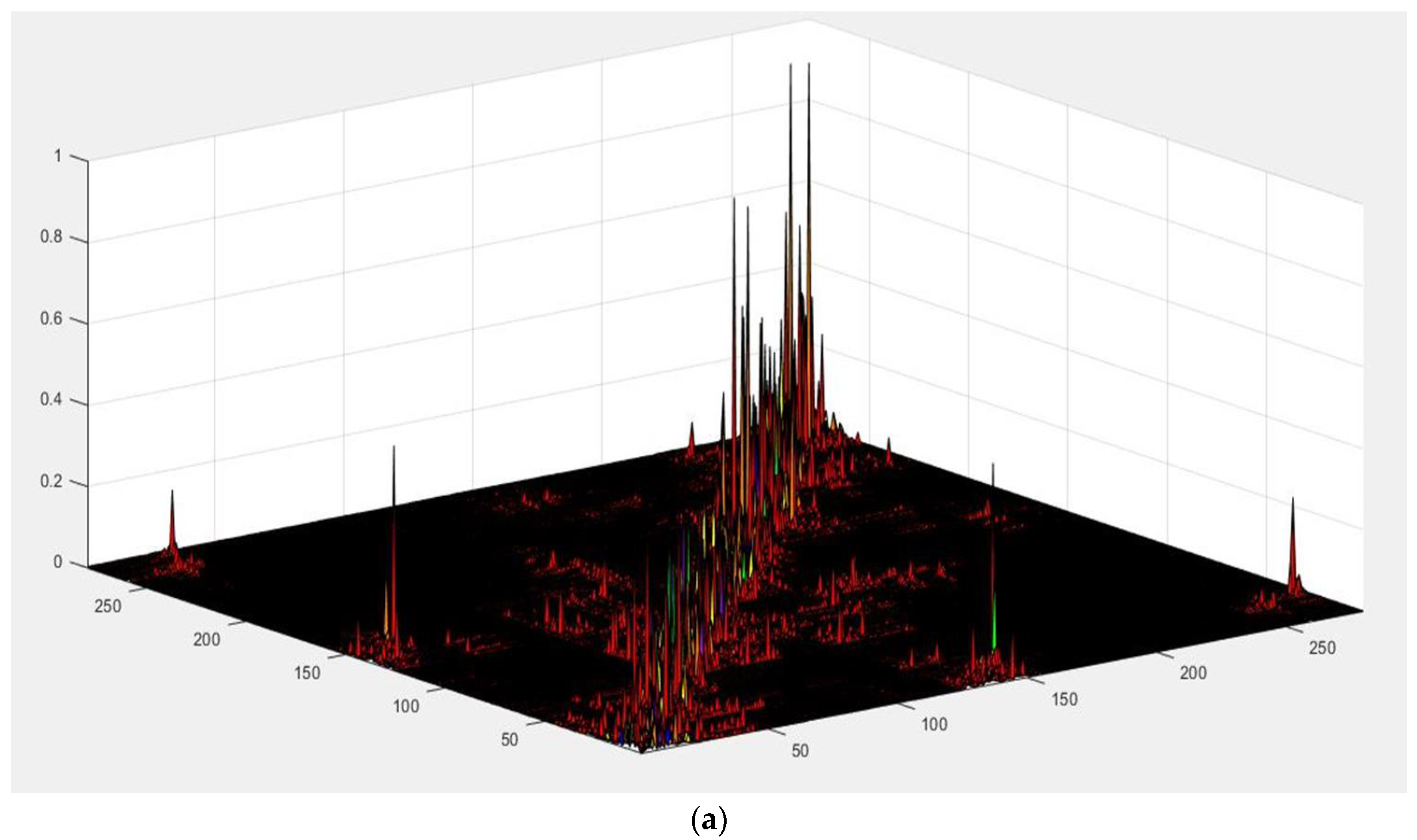
Figure 1. The weight matrices reflect spillover effects in 280 prefectural cities and their changes during 2003–2019. (a) Spatial weight matrix; (b) Changes in the spillover effects during different periods; (c) Spatiotemporal weight matrix. Note: this figure is drawn by MATLAB R2020a. In subgraph (a), the horizontal axis and the vertical axis both indicate 280 prefectural cities; in subgraph (b), the axes both indicate the years from 2003 to 2019; in subgraph (c), the axes both indicate the pooled series with 280 cities and 17 years sorted first by the cities and then the years.
Sustainability 15 00322 g001aSustainability 15 00322 g001b
Figure 2. Calculated results of China’s industrial TFPs at the prefectural level. Note: the figure is drawn by MATLAB R2020a; the horizontal axis indicates years from 2003 to 2019, and the vertical axis indicates 280 prefectural cities; the details of the order of the cities can be obtained from the author by email.
Sustainability 15 00322 g002
Figure 3. Mean values of industrial TFPs of China’s prefectural cities and their histogram fit. Note: the figure is drawn by MATLAB R2020a.
Sustainability 15 00322 g003
Figure 4. Dagum’s Gini coefficients of China’s industrial TFP at the prefectural level and their contribution decomposition with different spatial groups classified. Note: the figure is drawn by MATLAB R2020a.
Sustainability 15 00322 g004
Figure 5. Kernel density estimation of China’s industrial TFPs at the prefectural level. Note: the figure is drawn by MATLAB R2020a.
Sustainability 15 00322 g005
Table 1. Formulas of shares of capital and energy in China’s prefectural industrial sector under the different optimal models.
ModelsShare of Capital Inputs ( a ^ k , * )Share of Energy Inputs ( a ^ e n , * )
GNSM 1 N T T r a c e { [ Ω ^ 1 ( I N T β ^ 1 + S T W θ ^ 1 ) ] } 1 N T T r a c e { [ Ω ^ 1 ( I N T β ^ 2 + S T W θ ^ 2 ) ] }
SDM
SDEM 1 N T T r a c e ( I N T β ^ 1 + S T W θ ^ 1 ) 1 N T T r a c e ( I N T β ^ 2 + S T W θ ^ 2 )
SXL
SAC 1 N T T r a c e ( Ω ^ 1 β ^ 1 ) 1 N T T r a c e ( Ω ^ 1 β ^ 2 )
SAR
SEM β ^ 1 β ^ 2
NSM
Table 2. Descriptive statistics of related variables for calculating China’s industrial TFPs at the prefectural level.
Gross Value of Industrial Outputs
(100 Million Yuan)
Industrial Capital Stock
(100 Million Yuan)
Industrial Total Employed Persons
(10 Thousand)
Industrial Electricity Consumption
(100 Million kWh)
Mean200.41 239.67 15.48 107.15
Median121.62 137.56 9.43 65.66
Maximum2160.22 3984.01 260.92 1611.90
Minimum3.29 2.14 0.31 0.23
Std. Dev.235.51 291.34 20.73 133.45
Skewness2.93 3.04 5.15 4.15
Kurtosis14.66 18.42 43.34 30.69
Jarque-Bera3.38 × 1045.45 × 1043.44 × 1051.66 × 105
Probability0.0000 0.0000 0.0000 0.0000
Sum9.54 × 1051.14 × 1067.37 × 1045.10 × 105
Sum Sq. Dev.2.64 × 1084.04 × 1082.04 × 1068.48 × 107
Observations4760476047604760
Note: the results are obtained based on MATLAB R2020a and EVIEWS 11.0.
Table 3. Estimated results of eight spatial models without fixed effects and random effects.
NSMSXLSARSDMSEMSDEMSACGNSM
C o n s t . 1.8445
(66.69 ***)
1.1687
(22.76 ***)
−0.2521
(−5.62 ***)
0.2062
(43.22 ***)
20.414
(86.63 ***)
19.635
(119.43 ***)
1.3248
(9.76 ***)
2.4504
(6.14 ***)
L o g ( K / L ) 0.6128
(51.41 ***)
0.4774
(33.22 ***)
0.3498
(32.95 ***)
0.4552
(11.21 ***)
0.456
(66.62 ***)
0.4503
(43.41 ***)
0.4502
(41.21 ***)
0.4404
(40.07 ***)
L o g ( E / L ) 0.066
(6.04 ***)
0.0817
(7.26 ***)
0.0942
(10.89 ***)
0.0995
(7.95 ***)
0.0992
(11.42 ***)
0.1088
(12.07 ***)
0.1009
(11.77 ***)
0.1069
(11.86 ***)
S T W × L o g ( K / L ) 0.5161
(14.77 ***)
−0.4676
(−38.29 ***)
−0.0433
(−1.40)
−0.2676
(−4.91 ***)
S T W × L o g ( E / L ) −0.0748
(−2.40 **)
−0.0764
(−2.73 ***)
0.1013
(3.51 ***)
0.0964
(3.23 ***)
ρ 0 0.866
(53.58 ***)
0.9899
(33.58 ***)
−0.133
(−3.24 ***)
0.4004
(4.46 ***)
λ 0 0.99
(5040.3 ***)
0.99
(7078.2 ***)
1.2072
(64.20 ***)
0.9019
(43.24 ***)
R ^ 2 0.47880.5053−0.3163−520.13−0.31630.70440.71130.7032
σ 2 0.32650.30990.20370.18540.20370.18500.18070.1857
L o g ( L ) −4088.4−3963.1−1354.6−1123−1354.6−1117.7−1084.5−2771.7
Note: the above outputs were collected based on MATLAB R2020a. () represents T-statistic, ***, and ** mean having passed the hypothesis test with a significance level of 1%, and 5%.
Table 4. Estimated results of NSM and SXL models with fixed effects.
Individual Fixed Effects ModelsPeriod Fixed Effects ModelsIndividual and Period Fixed Effects Models
NSMSXLNSMSXLNSMSXL
L o g ( K / L ) 0.7186
(78.44 ***)
0.5919
(43.52 ***)
0.4581
(34.37 ***)
0.4104
(29.33 ***)
1.201
(137.28 ***)
0.5649
(44.53 ***)
L o g ( E / L ) 0.2062
(18.64 ***)
0.1417
(14.10 ***)
0.0563
(5.62 ***)
0.0792
(7.61 ***)
0.2058
(16.88 ***)
0.1202
(12.83 ***)
S T W × L o g ( K / L ) −0.8341
(−18.13 ***)
0.3987
(11.20 ***)
0.519
(9.75 ***)
S T W × L o g ( E / L ) 1.9307
(33.56 ***)
−0.1981
(−6.87 ***)
0.4655
(6.65 ***)
R ^ 2 0.73890.79270.28310.30160.0360.4504
σ 2 0.09690.07690.2650.25810.11030.0629
L o g ( L ) −1197.4−647.22−3592.1−3528.7−1505.1−166.79
Note: the above outputs were collected based on MATLAB R2020a. () represents T-statistic, *** means having passed the hypothesis test with a significance level of 1%.
Table 5. Relative changes in the kernel density estimation results.
YearAnalyzed RegionsBenchmark RegionsMovement Direction of the Distribution CurveKernel Density at the Peak PointDistribution RangeTails of the Distribution Curve
2003EasternCentralWidenExtend
WesternCentralAlmost the same-
NortheastWesternWiden-
2011EasternCentralAlmost the same-
WesternCentralAlmost the sameAlmost the sameExtend
NortheastWestern-Narrow
2019EasternCentralAlmost the same-Narrow
WesternCentral--
NortheastWesternAlmost the sameNarrowNarrow
Note: →, ←, ↓, and ↑ indicate moving rightwards, leftwards, downwards, and upwards.
Disclaimer/Publisher’s Note: The statements, opinions and data contained in all publications are solely those of the individual author(s) and contributor(s) and not of MDPI and/or the editor(s). MDPI and/or the editor(s) disclaim responsibility for any injury to people or property resulting from any ideas, methods, instructions or products referred to in the content.