
Optimal Power Flow with Stochastic Renewable Energy Using Three Mixture Component Distribution Functions

 ,
,  ,
, 
 and
and 
Abstract
:1. Introduction
- Using a novel MA method to estimate parameters of original and mixture distributions;
- Using a novel MA method to solve traditional OPF and SCOPF problems;
- Simulating stochastic behavior and renewable energy using TCMD in the SCOPF problem;
- Using the TCMD model to study the effect of changing scheduled power, renewable sources cost coefficients in the total cost of operation.
2. Renewable Energy Modeling
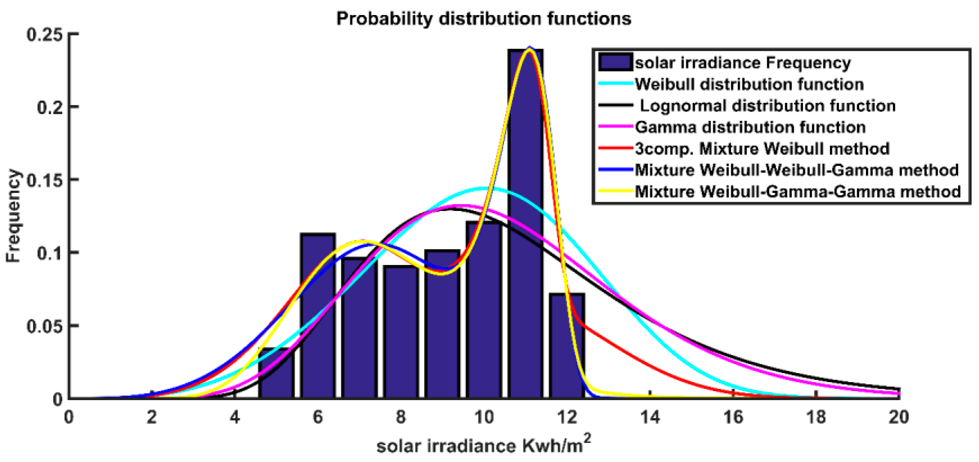
2.1. Wind Speed and Solar Irradiance Distribution Functions
2.2. Wind Power Distribution Function
2.3. Solar Power Distribution Functions
3. Optimal Power Flow
3.1. Single-Objective OPF Problem
3.2. Multi-Objective OPF Problem
3.3. Objective Functions
- (a)
- Fuel Cost
- (b)
- Wind and Solar Generation Cost
- (c)
- Active Power Losses
- (d)
- Voltage Security Index
- (e)
- Emission Function
- (f)
- Problem constraints
4. Mayfly Algorithm
4.1. MMA’ Movement
4.2. FMA’ Movement
4.3. Mating
4.4. Mutation
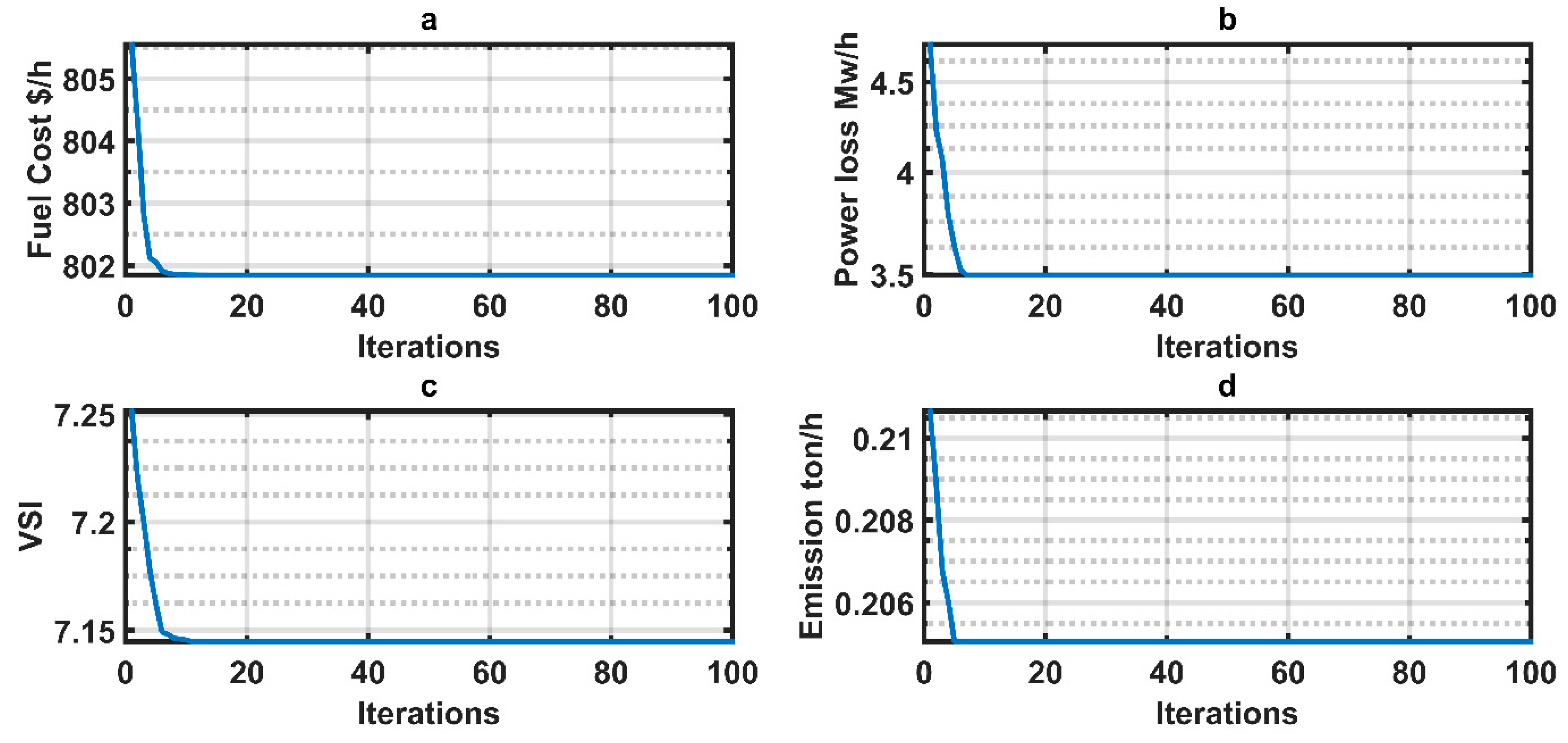
5. Results and Discussion
5.1. Case 1: Renewable Energy Modeling
5.2. Case 2: Optimal Power Flow
5.3. Case 3: Multi-Objective Optimal Power Flow
5.4. Case 4: Stochastic Optimal Power Flow
5.5. Case 5: Multi-Objective SCOPF
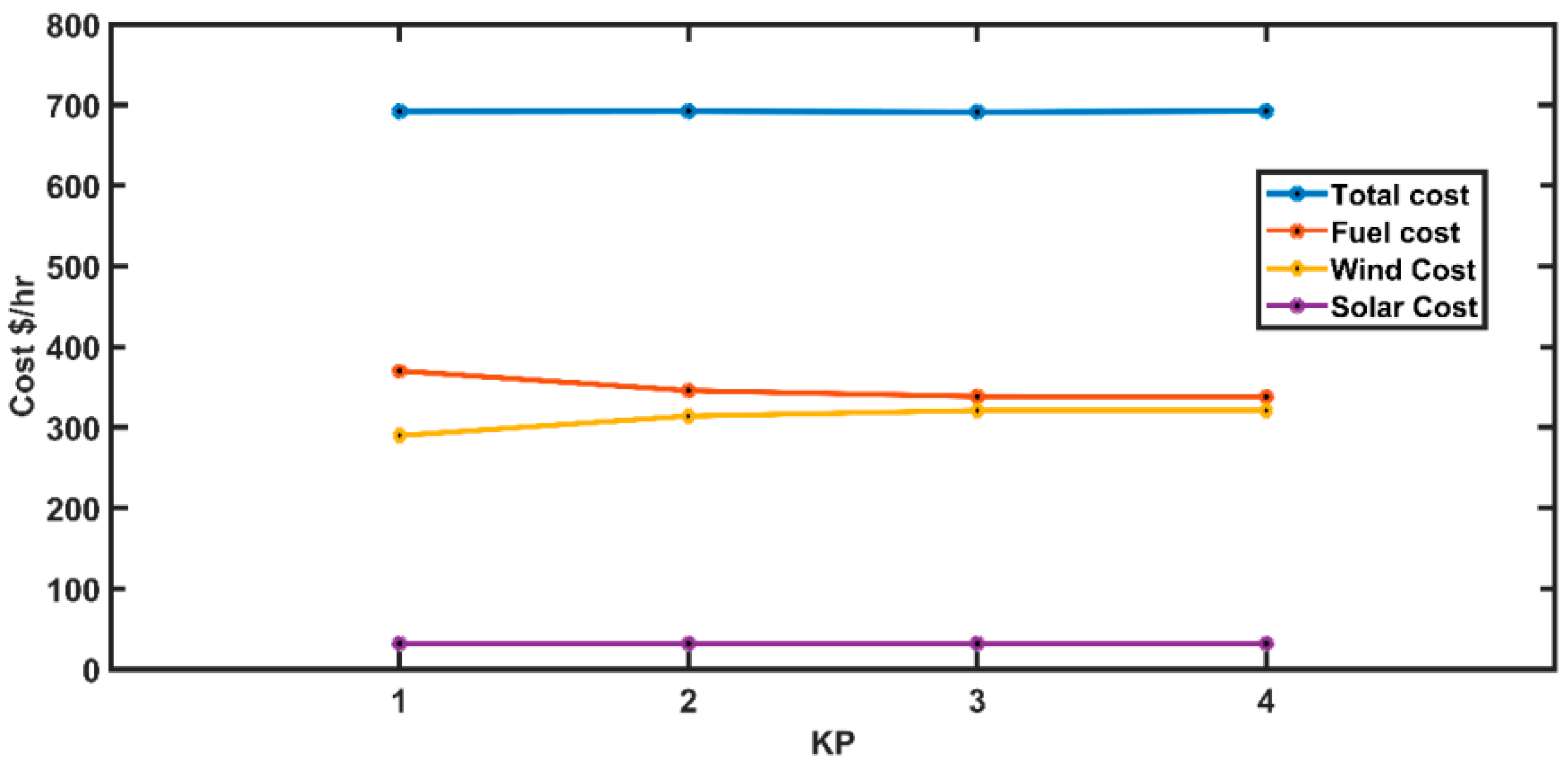
5.6. Case 6: Wind and Solar Generation Costs versus Penalty Cost Coefficient
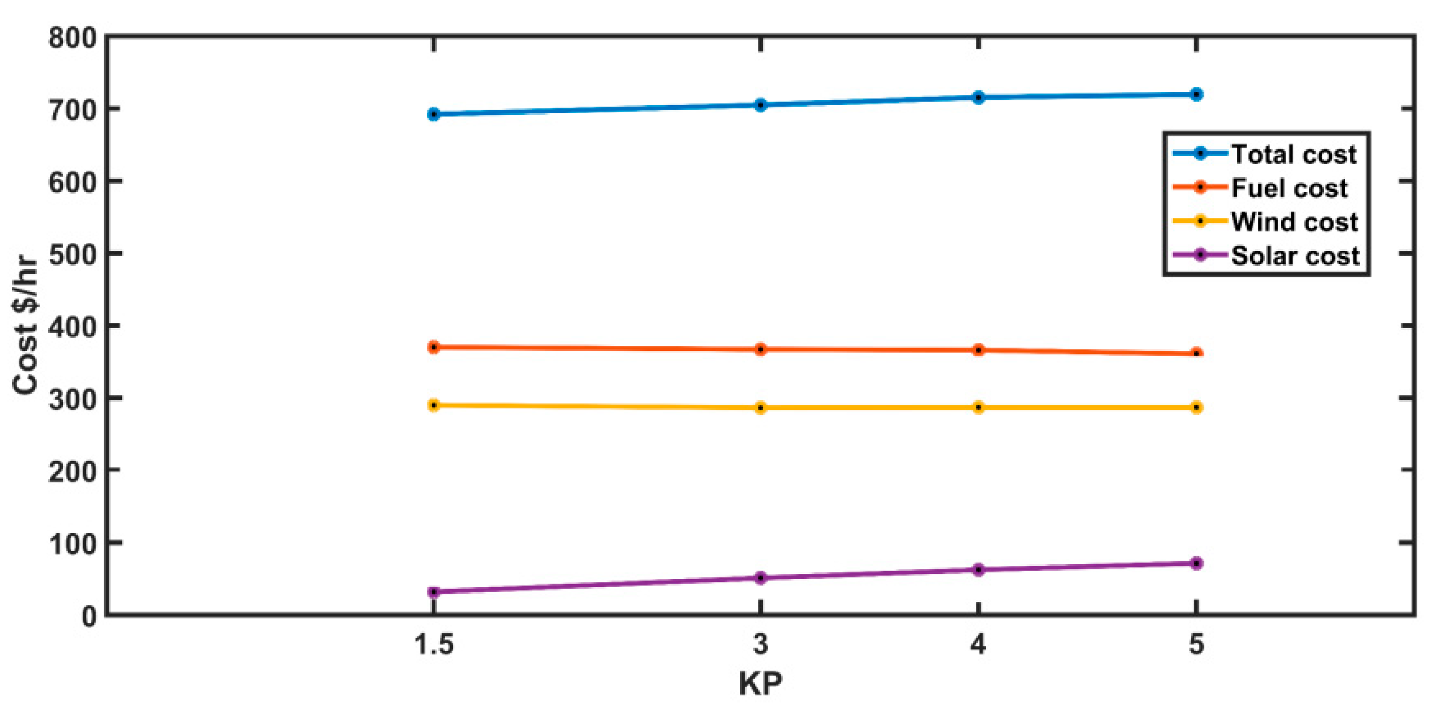
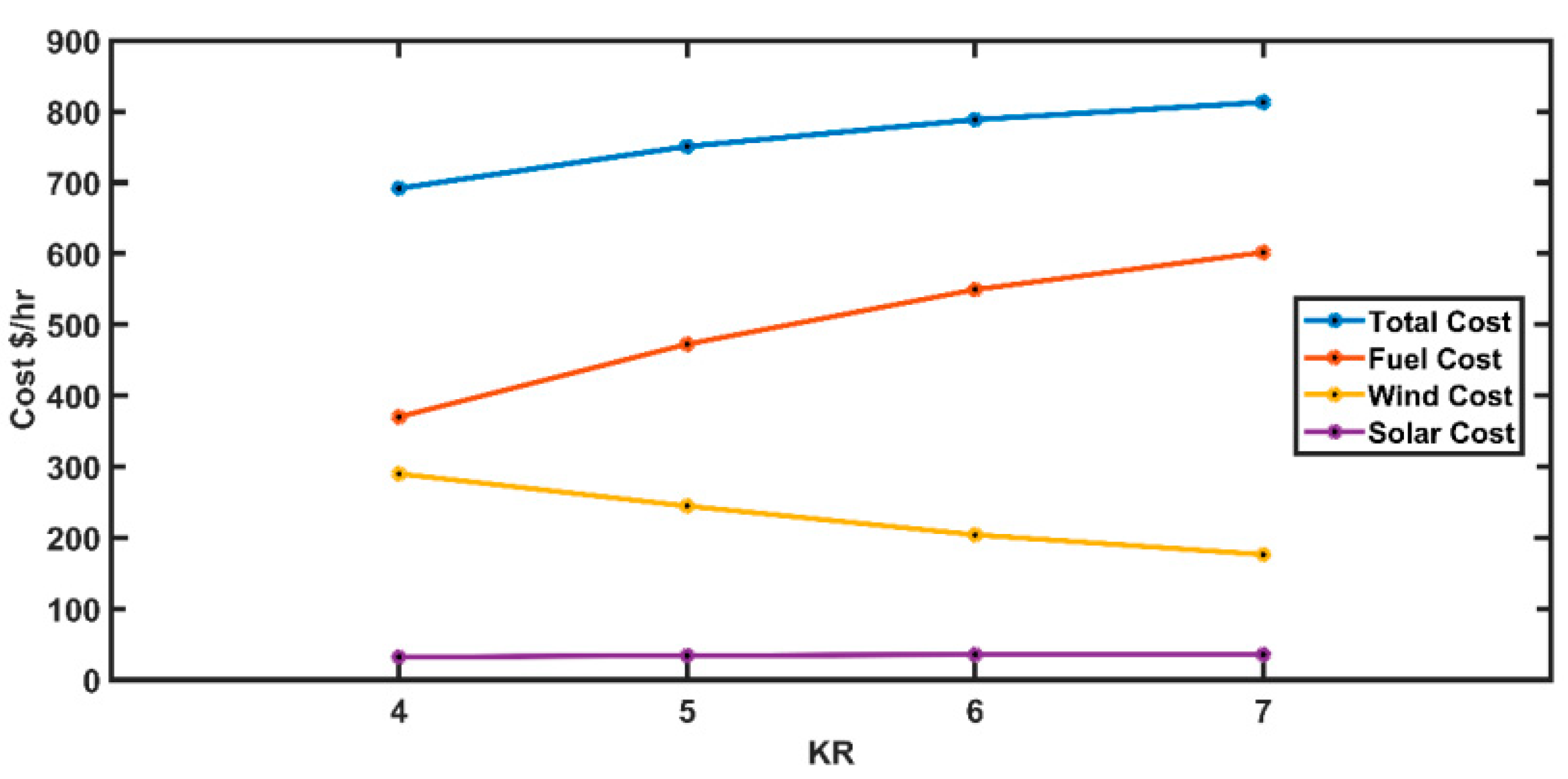
5.7. Case 7: Wind and Solar Generation Costs versus Reserve Cost Coefficient
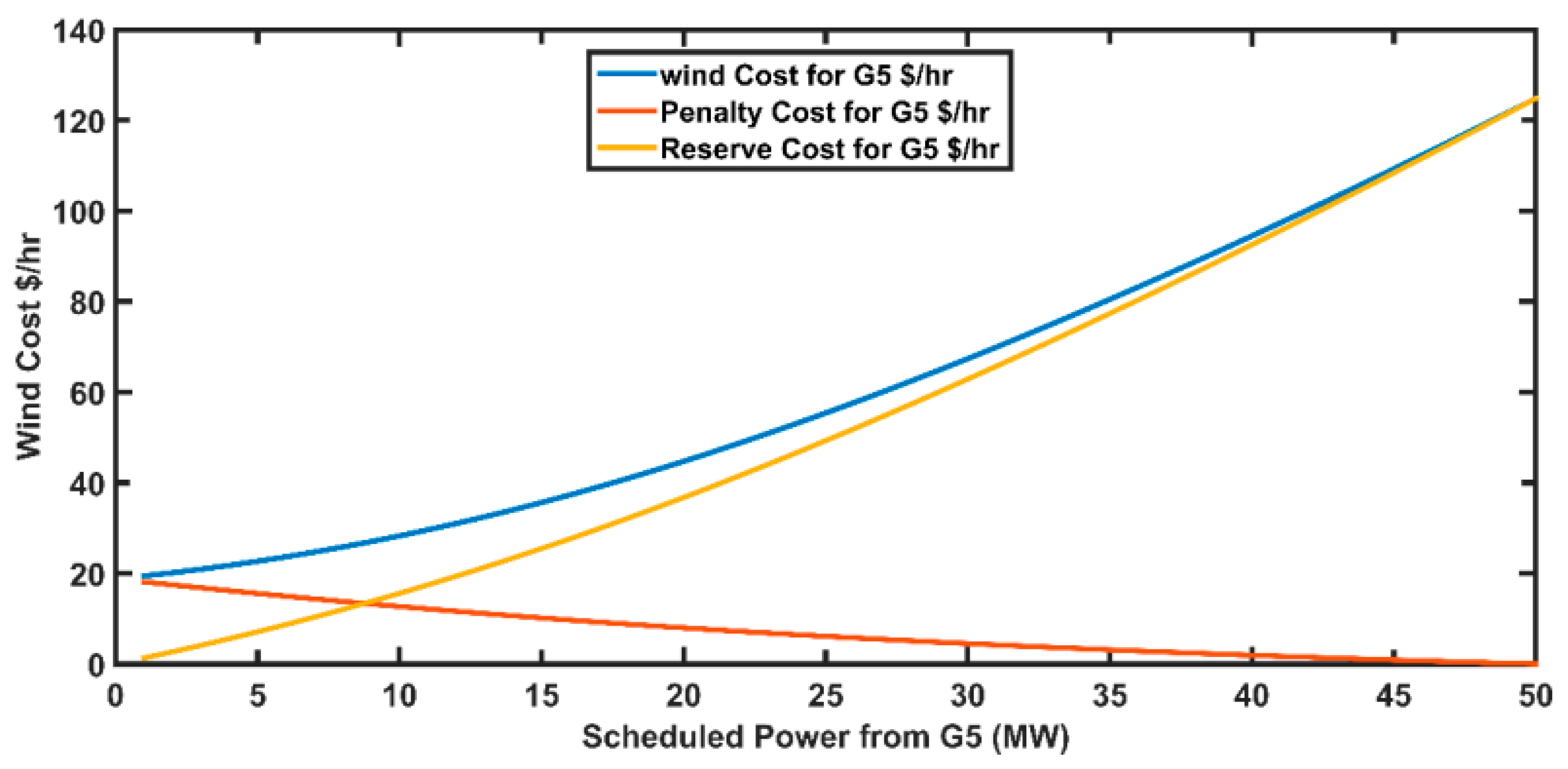
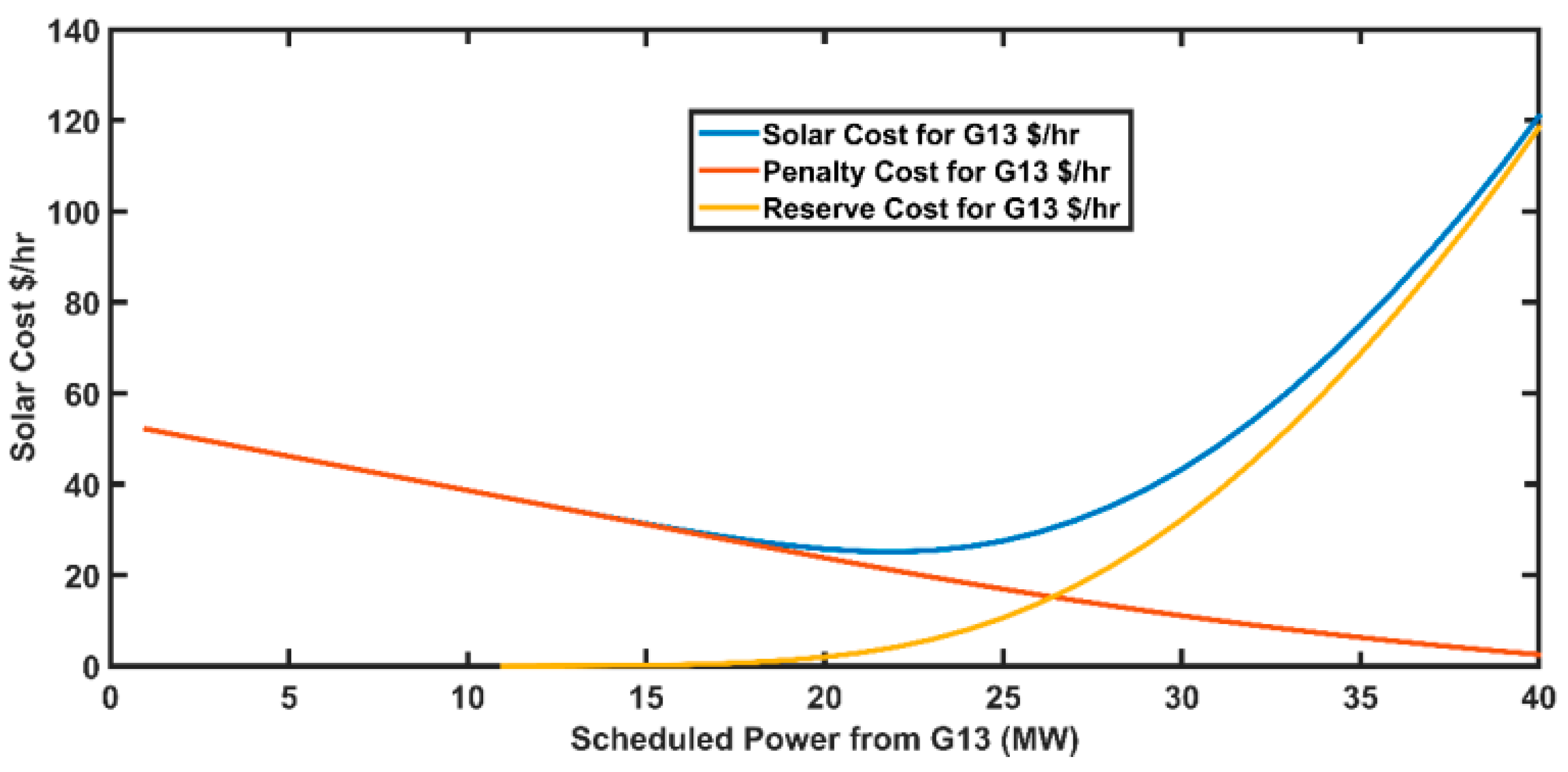
5.8. Case 8: Wind and Solar Generation Cost versus Scheduled Power by the Operator
6. Conclusions
Author Contributions
Funding
Data Availability Statement
Conflicts of Interest
References
- Luna-Rubio, R.; Trejo-Perea, M.; Vargas-Vázquez, D.; Ríos-Moreno, G. Optimal sizing of renewable hybrids energy systems: A review of methodologies. Sol. Energy 2012, 86, 1077–1088. [Google Scholar] [CrossRef]
- Erdinc, O.; Uzunoglu, M. Optimum design of hybrid renewable energy systems: Overview of different approaches. Renew. Sustain. Energy Rev. 2012, 16, 1412–1425. [Google Scholar] [CrossRef]
- Chauhan, A.; Saini, R. A review on Integrated Renewable Energy System based power generation for stand-alone applications: Configurations, storage options, sizing methodologies and control. Renew. Sustain. Energy Rev. 2014, 38, 99–120. [Google Scholar] [CrossRef]
- Spiecker, S.; Weber, C. The future of the European electricity system and the impact of fluctuating renewable energy–A scenario analysis. Energy Policy 2014, 65, 185–197. [Google Scholar] [CrossRef]
- Abdelaziz, A.Y.; El-Sharkawy, M.A.; Attia, M.A.; Panigrahi, B.K. Genetic algorithm based approach for optimal allocation of TCSC for power system loadability enhancement. In International Conference on Swarm, Evolutionary, and Memetic Computing; Springer: Berlin/Heidelberg, Germany, 2012. [Google Scholar]
- Gooding, P.; Makram, E.; Hadidi, R. Probability analysis of distributed generation for island scenarios utilizing Carolinas data. Electr. Power Syst. Res. 2014, 107, 125–132. [Google Scholar] [CrossRef]
- Khamees, A.K.; Abdelaziz, A.Y.; Eskaros, M.R.; El-Shahat, A.; Attia, M.A. Optimal Power Flow Solution of Wind-Integrated Power System Using Novel Metaheuristic Method. Energies 2021, 14, 6117. [Google Scholar] [CrossRef]
- Khamees, A.K.; Abdelaziz, A.Y.; Eskaros, M.R.; Alhelou, H.H.; Attia, M.A. Stochastic Modeling for Wind Energy and Multi-Objective Optimal Power Flow by Novel Meta-Heuristic Method. IEEE Access 2021, 9, 158353–158366. [Google Scholar] [CrossRef]
- Thevenard, D.; Pelland, S. Estimating the uncertainty in long-term photovoltaic yield predictions. Sol. Energy 2013, 91, 432–445. [Google Scholar] [CrossRef]
- Sameh, M.A.; Badr, M.A.; Mare, M.I.; Attia, M.A. Enhancing the performance of photovoltaic systems under partial shading conditions using cuttlefish algorithm. In Proceedings of the 2019 8th International Conference on Renewable Energy Research and Applications (ICRERA), IEEE, Brasov, Romania, 3–6 November 2019. [Google Scholar]
- Omar, O.A.; Badra, N.M.; Attia, M.A. Enhancement of on-grid pv system under irradiance and temperature variations using new optimized adaptive controller. Int. J. Electr. Comput. Eng. 2018, 8, 2650. [Google Scholar] [CrossRef]
- Dommel, H.W.; Tinney, W.F. Optimal power flow solutions. IEEE Trans. Power Appar. Syst. 1968, 1866–1876. [Google Scholar] [CrossRef]
- Li, S.; Gong, W.; Wang, L.; Yan, X.; Hu, C. Optimal power flow by means of improved adaptive differential evolution. Energy 2020, 198, 117314. [Google Scholar] [CrossRef]
- Nguyen, T.T. A high performance social spider optimization algorithm for optimal power flow solution with single objective optimization. Energy 2019, 171, 218–240. [Google Scholar] [CrossRef]
- Yuan, X.; Zhang, B.; Wang, P.; Liang, J.; Yuan, Y.; Huang, Y.; Lei, X. Multi-objective optimal power flow based on improved strength Pareto evolutionary algorithm. Energy 2017, 122, 70–82. [Google Scholar] [CrossRef]
- Naderi, E.; Pourakbari-Kasmaei, M.; Cerna, F.V.; Lehtonen, M. A novel hybrid self-adaptive heuristic algorithm to handle single-and multi-objective optimal power flow problems. Int. J. Electr. Power Energy Syst. 2021, 125, 106492. [Google Scholar] [CrossRef]
- Jiang, P.; Li, R.; Li, H. Multi-objective algorithm for the design of prediction intervals for wind power forecasting model. Appl. Math. Model. 2019, 67, 101–122. [Google Scholar] [CrossRef]
- Zervoudakis, K.; Tsafarakis, S. A mayfly optimization algorithm. Comput. Ind. Eng. 2020, 145, 106559. [Google Scholar] [CrossRef]
- Islam, M.; Saidur, R.; Rahim, N. Assessment of wind energy potentiality at Kudat and Labuan, Malaysia using Weibull distribution function. Energy 2011, 36, 985–992. [Google Scholar] [CrossRef]
- Carta, J.; Ramirez, P. Analysis of two-component mixture Weibull statistics for estimation of wind speed distributions. Renew. Energy 2007, 32, 518–531. [Google Scholar] [CrossRef]
- Van der Auwera, L.; de Meyer, F.; Malet, L. The use of the Weibull three-parameter model for estimating mean wind power densities. J. Appl. Meteorol. Climatol. 1980, 19, 819–825. [Google Scholar] [CrossRef]
- Carta, J.A.; Ramírez, P. Use of finite mixture distribution models in the analysis of wind energy in the Canarian Archipelago. Energy Convers. Manag. 2007, 48, 281–291. [Google Scholar] [CrossRef]
- Celik, A.N. Energy output estimation for small-scale wind power generators using Weibull-representative wind data. J. Wind. Eng. Ind. Aerodyn. 2003, 91, 693–707. [Google Scholar] [CrossRef]
- Khamees, A.K.; Abdelaziz, A.Y.; Ali, Z.M.; Alharthi, M.M.; Ghoneim, S.S.; Eskaros, M.R.; Attia, M.A. Mixture probability distribution functions using novel metaheuristic method in wind speed modeling. Ain Shams Eng. J. 2022, 13, 101613. [Google Scholar] [CrossRef]
- Arevalo, J.C.; Santos, F.; Rivera, S. Uncertainty cost functions for solar photovoltaic generation, wind energy generation, and plug-in electric vehicles: Mathematical expected value and verification by Monte Carlo simulation. Int. J. Power Energy Convers. 2019, 10, 171–207. [Google Scholar] [CrossRef]
- Khamees, A.K.; Badra, N.; Abdelaziz, A.Y. Optimal power flow methods: A comprehensive survey. Int. Electr. Eng. J. 2016, 7, 2228–2239. [Google Scholar]
- Pan, X.; Chen, M.; Zhao, T.; Low, S.H. DeepOPF: A feasibility-optimized deep neural network approach for AC optimal power flow problems. IEEE Syst. J. 2022, 1–11. [Google Scholar] [CrossRef]
- Hazra, J.; Sinha, A. A multi-objective optimal power flow using particle swarm optimization. Eur. Trans. Electr. Power 2011, 21, 1028–1045. [Google Scholar] [CrossRef]
- Basu, M. Multi-objective optimal power flow with FACTS devices. Energy Convers. Manag. 2011, 52, 903–910. [Google Scholar] [CrossRef]
- Kumari, M.S.; Maheswarapu, S. Enhanced genetic algorithm based computation technique for multi-objective optimal power flow solution. Int. J. Electr. Power Energy Syst. 2010, 32, 736–742. [Google Scholar] [CrossRef]
- Khunkitti, S.; Siritaratiwat, A.; Premrudeepreechacharn, S.; Chatthaworn, R.; Watson, N.R. A hybrid DA-PSO optimization algorithm for multiobjective optimal power flow problems. Energies 2018, 11, 2270. [Google Scholar] [CrossRef] [Green Version]
- Al Alahmadi, A.A.; Belkhier, Y.; Ullah, N.; Abeida, H.; Soliman, M.S.; Khraisat, Y.S.H.; Alharbi, Y.M. Hybrid wind/PV/battery energy management-based intelligent non-integer control for smart DC-microgrid of smart university. IEEE Access 2021, 9, 98948–98961. [Google Scholar] [CrossRef]
- Althobaiti, A.; Ullah, N.; Belkhier, Y.; Babqi, A.J.; Alkhammash, H.I.; Ibeas, A. Expert knowledge based proportional resonant controller for three phase inverter under abnormal grid conditions. Int. J. Green Energy 2022, 1–17. [Google Scholar] [CrossRef]
- Summers, T.; Warrington, J.; Morari, M.; Lygeros, J. Stochastic optimal power flow based on conditional value at risk and distributional robustness. Int. J. Electr. Power Energy Syst. 2015, 72, 116–125. [Google Scholar] [CrossRef]
- Shi, L.; Wang, C.; Yao, L.; Ni, Y.; Bazargan, M. Optimal power flow solution incorporating wind power. IEEE Syst. J. 2011, 6, 233–241. [Google Scholar] [CrossRef]
- Kathiravan, R.; Kumudini Devi, R.P. Optimal power flow model incorporating wind, solar, and bundled solar-thermal power in the restructured Indian power system. Int. J. Green Energy 2017, 14, 934–950. [Google Scholar] [CrossRef]
- Available online: https://www.ncdc.noaa.gov/ (accessed on 1 January 2020).
- Wilcox, S. National Solar Radiation Database 1991–2010 Update; National Renewable Energy Laboratory, US Department of Energy: Washington, DC, USA, 2012.
- Weibull, W. A statistical distribution function of wide applicability. J. Appl. Mech. 1951, 18, 293–297. [Google Scholar] [CrossRef]
- Johnson, N.L.; Kotz, S.; Balakrishnan, N. Continuous Univariate Distributions, Volume 2; John Wiley & Sons: Hoboken, NJ, USA, 1995; Volume 289. [Google Scholar]
- Morgan, V.T. Statistical distributions of wind parameters at Sydney, Australia. Renew. Energy 1995, 6, 39–47. [Google Scholar] [CrossRef]
- Sarkar, A.; Behera, D.K. Wind turbine blade efficiency and power calculation with electrical analogy. Int. J. Sci. Res. Publ. 2012, 2, 1–5. [Google Scholar]
- Santana-Quintero, L.V.; Coello, C.A.C. An algorithm based on differential evolution for multi-objective problems. Int. J. Comput. Intell. Res. 2005, 1, 151–169. [Google Scholar] [CrossRef]
- Biswas, P.P.; Suganthan, P.; Amaratunga, G.A. Optimal power flow solutions incorporating stochastic wind and solar power. Energy Convers. Manag. 2017, 148, 1194–1207. [Google Scholar] [CrossRef]
- Omitaomu, O.A.; Niu, H. Artificial intelligence techniques in smart grid: A survey. Smart Cities 2021, 4, 548–568. [Google Scholar] [CrossRef]
- Zimmerman, R.D.; Murillo-Sánchez, C.E.; Gan, D. Matpower. PSERC.[Online]. Software. 1997. Available online: http://www.pserc.cornell.edu/matpower (accessed on 1 January 2020).
- Niknam, T.; Narimani, M.; Aghaei, J.; Azizipanah-Abarghooee, R. Improved particle swarm optimisation for multi-objective optimal power flow considering the cost, loss, emission and voltage stability index. IET Gener. Transm. Distrib. 2012, 6, 515–527. [Google Scholar] [CrossRef]
- Sivasubramani, S.; Swarup, K. Multi-objective harmony search algorithm for optimal power flow problem. Int. J. Electr. Power Energy Syst. 2011, 33, 745–752. [Google Scholar] [CrossRef]
- El-Fergany, A.A.; Hasanien, H.M. Single and multi-objective optimal power flow using grey wolf optimizer and differential evolution algorithms. Electr. Power Compon. Syst. 2015, 43, 1548–1559. [Google Scholar] [CrossRef]
- Khamees, A.K.; El-Rafei, A.; Badra, N.; Abdelaziz, A.Y. Solution of optimal power flow using evolutionary-based algorithms. Int. J. Eng. Sci. Technol. 2017, 9, 55–68. [Google Scholar] [CrossRef] [Green Version]
- Sayah, S.; Zehar, K. Modified differential evolution algorithm for optimal power flow with non-smooth cost functions. Energy Convers. Manag. 2008, 49, 3036–3042. [Google Scholar] [CrossRef]
- Bouzeboudja, H.; Chaker, A.; Allali, A.; Naama, B. Economic dispatch solution using a real-coded genetic algorithm. Acta Electrotech. Inform. 2005, 5, 4. [Google Scholar]
- Niknam, T.; Narimani, M.R.; Jabbari, M.; Malekpour, A.R. A modified shuffle frog leaping algorithm for multi-objective optimal power flow. Energy 2011, 36, 6420–6432. [Google Scholar] [CrossRef]


| Distribution Name | Equation | Distribution Parameters | |
|---|---|---|---|
| WD [39]. | (1) | k shape parameter c scale parameter | |
| LD [40]. | (2) | mean standard deviation | |
| GD [41] | (3) | a shape parameter b scale parameter | |
| Distribution Name | Equation | |
|---|---|---|
| Mixture WD | (4) | |
| Mixture WD-WD-GD | (5) | |
| Mixture WD-GD-GD | (6) | |
| Wind Speed Modeling | Solar Irradiance Modeling | |||
|---|---|---|---|---|
| Probability Distribution Function | Parameters | RMSE | Parameters | RMSE |
| WD | k = 1.72 c = 3.39 | 0.0062 | k = 4.08 c = 10.77 | 0.046732 |
| LD | = 1.15 = 1 | 0.0249 | = 2.31 = 0.31 | 0.052494 |
| LG | a = 2.60 b = 1.23 | 0.0038 | a = 10.96 b = 0.94 | 0.050583 |
| Mixture WD | C1 = 5.21 K1 = 2.14 C2 = 2.62 K2 = 1.94 C3 = 2.94 K3 = 10 W1 = 0.39 W2 = 0.59 | 0.00109 | C1 = 6.91 K1 = 5.13 C2 = 10.75 K2 = 4.13 C3 = 11.11 K3 = 20 W1 = 0.24 W2 = 0.5 | 0.013409 |
| Mixture WD-WD-GD | C1 = 5.33 K1 = 2.01 C2 = 3.03 K2 = 5.24 a = 2.72 b = 1 W1 = 0.27 W2 = 0.05 | 0.000736 | C1 = 11.18 K1 = 17.03 C2 = 7.80 K2 = 4.33 a = 15.43 b = 17.26 W1 = 0.412 W2 = 0.5 | 0.014118 |
| Mixture WD-GD-GD | C1 = 3.02 K1 = 5.27 a1 = 5.62 b1 = 1 a2 = 2.74 b2 = 1 W1 = 0.05 W2 = 0.19 | 0.00068 | C = 11.16 K = 17.07 a1 = 15.63 b1 = 0.482 a2 = 15.46 b2 = 8.34 W1 = 0.394 W2 = 0.498 | 0.012515 |
| Objective Function | Fuel Cost ($/h) | Power Loss (MW) | VSI | Emission (ton/h) |
|---|---|---|---|---|
| 176.7 | 51.9 | 177.5 | 64.3 | |
| 48.8 | 80 | 20 | 67.7 | |
| 21.5 | 50 | 15 | 50 | |
| 21.6 | 30 | 10 | 35 | |
| 12 | 35 | 30 | 30 | |
| 12 | 40 | 40 | 40 | |
| Fuel Cost | 801.8 | 968.6 | 849.9 | 945.5 |
| Power Loss | 9.4 | 3.5 | 9.1 | 3.6 |
| VSI | 7.6 | 7.2 | 7.1 | 7.2 |
| Emission | 0.4 | 0.2 | 0.4 | 0.2 |
| Technique | Emissions Minimization ($/h) |
|---|---|
| MA | 0.2050 |
| GA [47] | 0.20723 |
| PSO [47] | 0.2063 |
| Improved PSO [47] | 0.2058 |
| Technique | Power Loss minimization (MW/h) |
| MA | 3.49 |
| Harmony search algorithm [48] | 3.51 |
| GA [30] | 3.62 |
| Technique | VSI minimization |
| MA | 7.1449 |
| DE [49] | 8.2367 |
| GWO [49] | 8.268 |
| Method | Fuel Cost Minimization ($/h) |
|---|---|
| MA | 801.84 |
| Gray wolf optimizer (GWO) [50] | 801.86 |
| DE [51] | 802.39 |
| GA [52] | 801.96 |
| Shuffled frog leaping algorithm [53] | 802.51 |
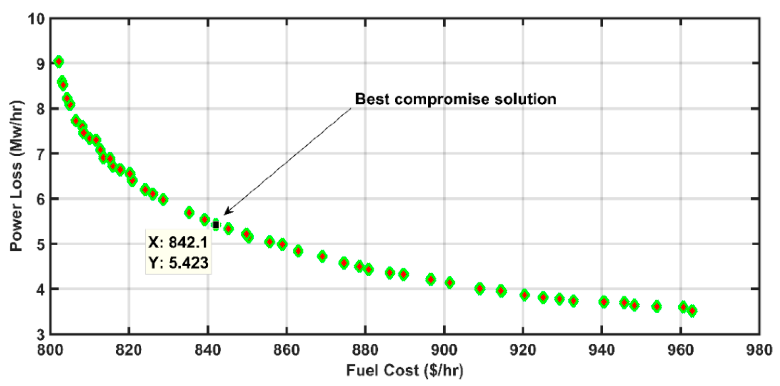
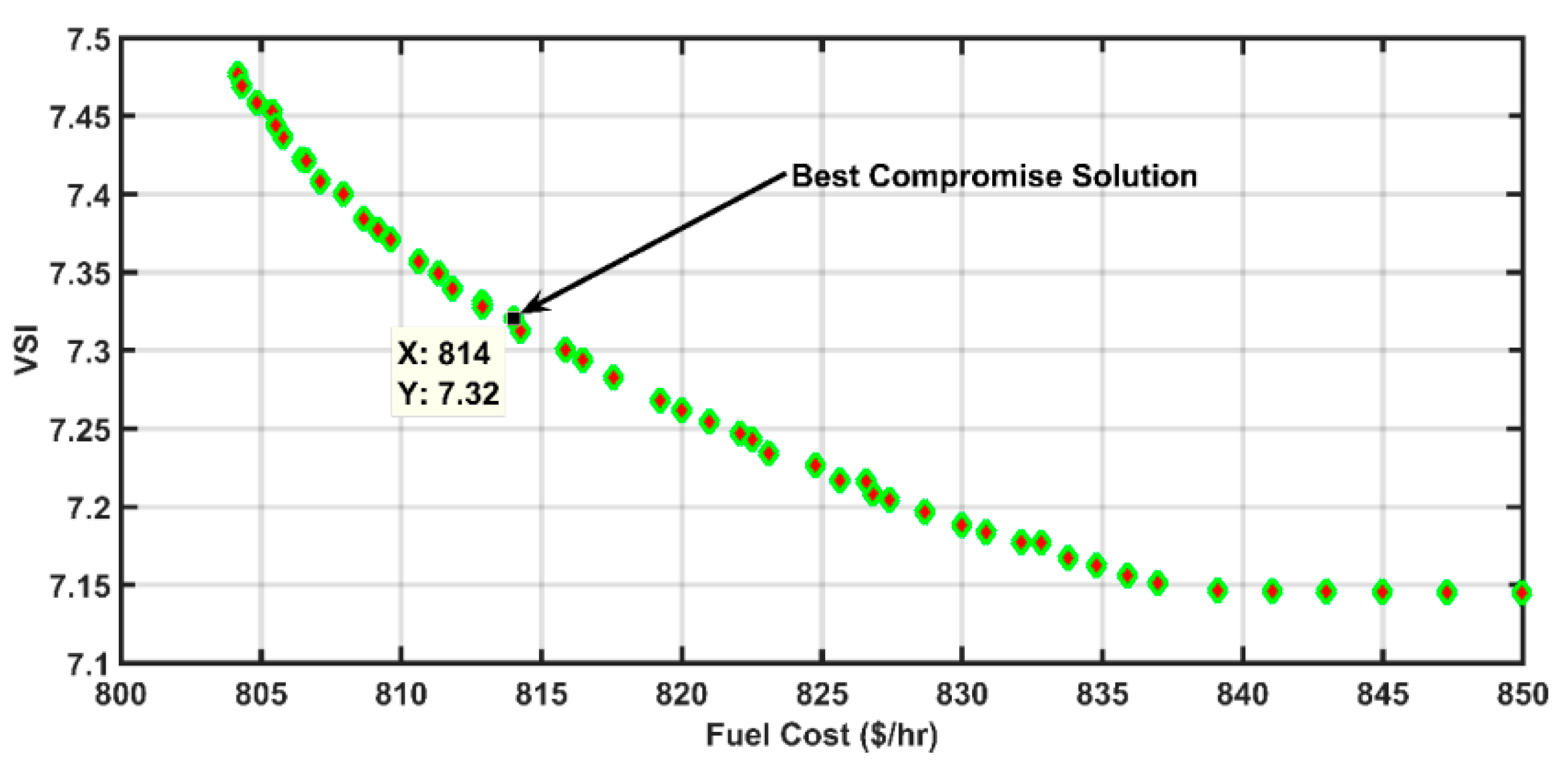
| Objective Functions | Fuel Cost-Power Loss | Fuel Cost-VSI | Fuel Cost-Emission |
|---|---|---|---|
| 112.49 | 163.50 | 112.61 | |
| 56.36 | 46.47 | 58.67 | |
| 33.41 | 19.42 | 29.23 | |
| 34.43 | 11.00 | 34.73 | |
| 27.66 | 24.81 | 25.85 | |
| 24.47 | 26.80 | 27.94 | |
| Fuel Cost | 842.06 | 814.25 | 838.81 |
| Power Loss | 5.42 | 8.59 | 5.64 |
| VSI | 7.36 | 7.33 | 7.34 |
| Emission | 0.24 | 0.33 | 0.24 |
| Objective Function | Total Cost ($/h) | Power Loss (MW) | VSI | Emission (ton/h) |
|---|---|---|---|---|
| 51.90 | 51.90 | 200.00 | 51.90 | |
| 80.00 | 80.00 | 0.00 | 80.00 | |
| 50.00 | 50.00 | 0.00 | 50.00 | |
| 35.00 | 35.00 | 10.00 | 35.00 | |
| 30.00 | 30.00 | 30.00 | 30.00 | |
| 40.00 | 40.00 | 40.00 | 40.00 | |
| Fuel cost | 370.07 | 350.31 | 2226.29 | 350.31 |
| Wind Power Cost | 289.87 | 319.95 | 48.79 | 321.54 |
| Solar Power Cost | 32.03 | 122.89 | 123.12 | 124.48 |
| Total Cost | 691.96 | 793.15 | 2398.20 | 796.33 |
| Power Loss | 6.40 | 3.50 | 11.90 | 3.50 |
| VSI | 7.46 | 7.21 | 7.14 | 7.21 |
| Emission | 0.17 | 0.11 | 0.33 | 0.11 |
| Objective Functions | Total Cost-Power Loss | Total Cost-VSI | Total Cost-Emission |
|---|---|---|---|
| 74.33 | 133.90 | 76.49 | |
| 79.94 | 70.63 | 79.99 | |
| 49.99 | 6.97 | 49.99 | |
| 35.00 | 10.00 | 30.33 | |
| 23.32 | 30.00 | 26.53 | |
| 24.92 | 40.00 | 24.23 | |
| Fuel cost | 376.86 | 480.85 | 378.33 |
| Wind Power Cost | 317.85 | 195.04 | 322.75 |
| Solar Power Cost | 28.46 | 124.44 | 26.12 |
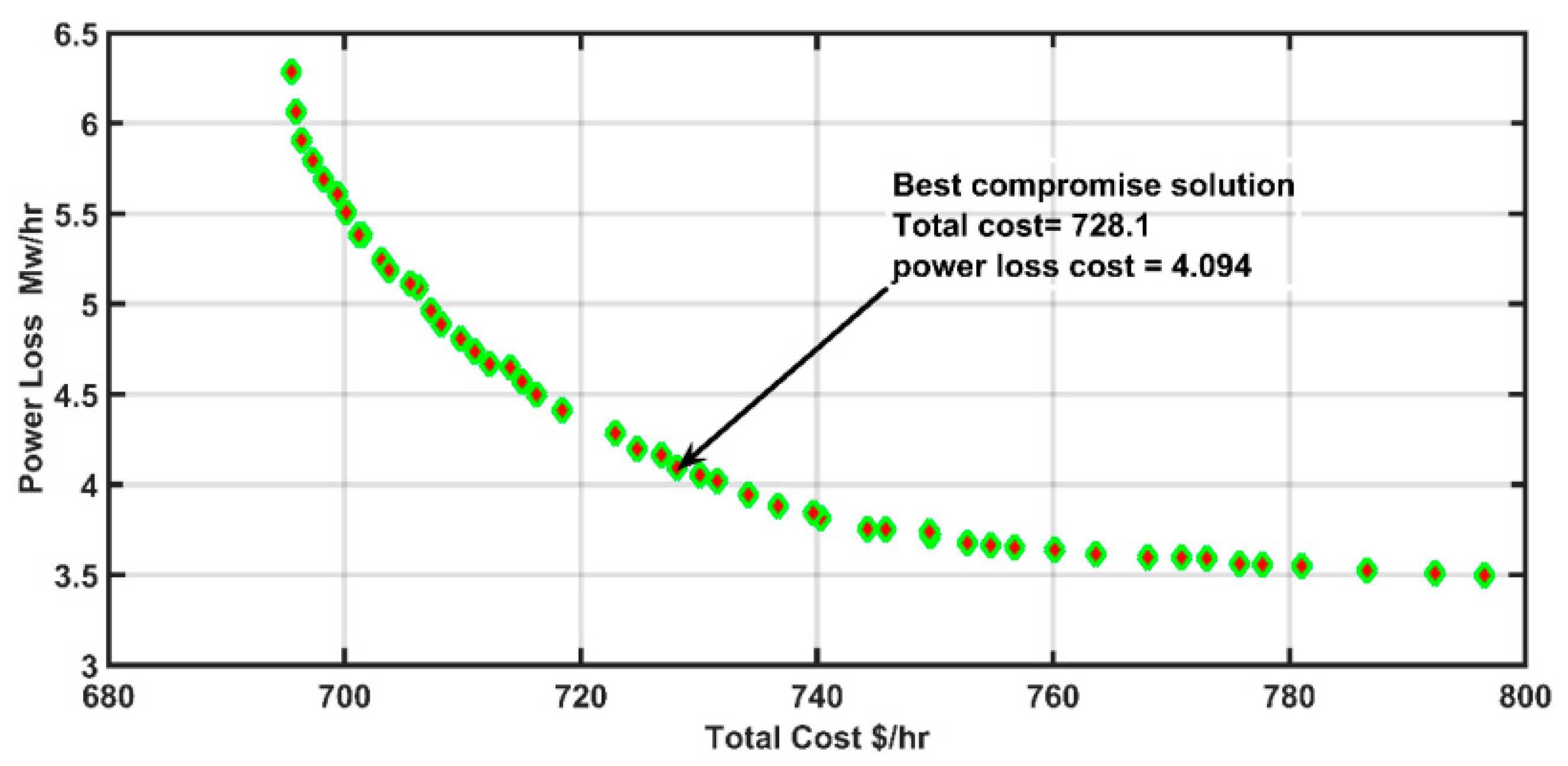
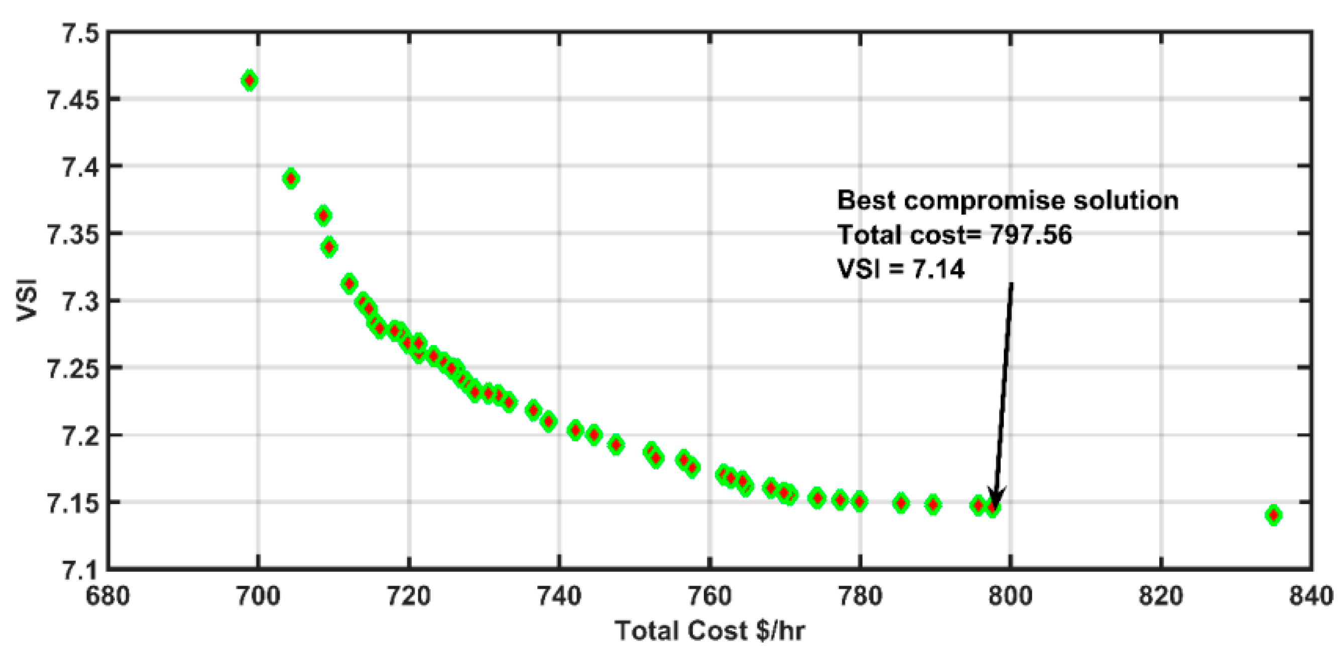
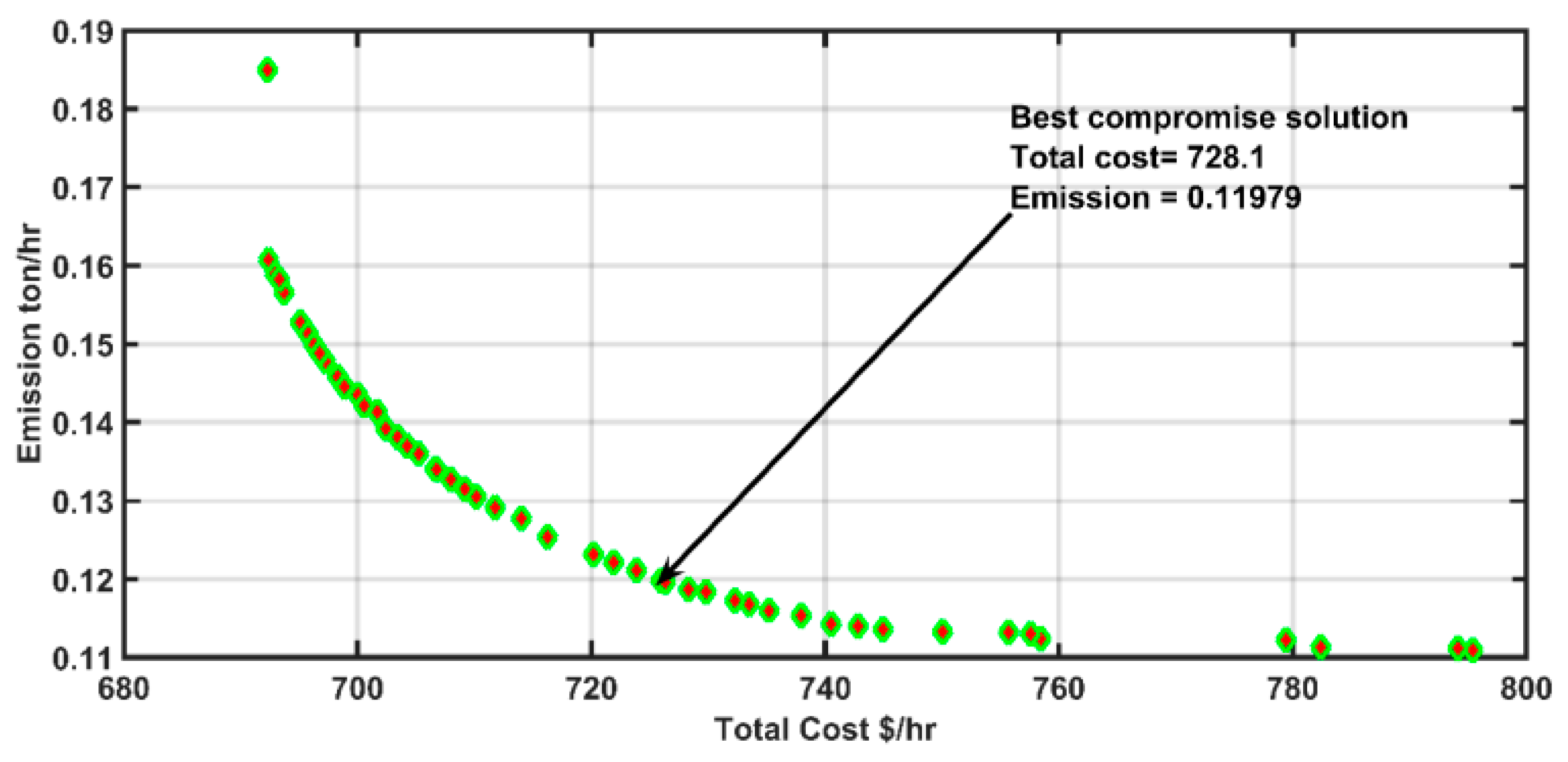
| Total Cost | 728.17 | 797.56 | 728.20 |
| Power Loss | 4.09 | 8.09 | 4.17 |
| VSI | 7.41 | 7.15 | 7.38 |
| Emission | 0.12 | 0.18 | 0.12 |
| 1 | 2 | 3 | 4 | |
|---|---|---|---|---|
| Fuel Cost | 370.07 | 345.60 | 338.37 | 338.18 |
| Wind Power Cost | 289.87 | 314.26 | 321.07 | 321.53 |
| Solar Power Cost | 32.03 | 32.32 | 31.99 | 32.62 |
| Total Cost | 691.96 | 692.18 | 691.43 | 692.34 |
| 1.5 | 3 | 4 | 5 | |
|---|---|---|---|---|
| Fuel cost | 370.07 | 367.13 | 366.01 | 360.98 |
| Wind Power Cost | 289.87 | 286.48 | 286.81 | 286.84 |
| Solar Power Cost | 32.03 | 51.13 | 62.42 | 71.56 |
| Total Cost | 691.96 | 704.74 | 715.24 | 719.38 |
| 4 | 5 | 6 | 7 | |
|---|---|---|---|---|
| Fuel Cost | 370.07 | 472.45 | 549.32 | 601.65 |
| Wind Power Cost | 289.87 | 244.50 | 204.00 | 176.15 |
| Solar Power Cost | 32.03 | 33.95 | 35.34 | 35.26 |
| Total Cost | 691.96 | 750.89 | 788.66 | 813.06 |
| 10 | 20 | 30 | 40 | |
|---|---|---|---|---|
| Fuel cost | 357.59 | 370.07 | 369.89 | 377.04 |
| Wind Power Cost | 281.46 | 289.87 | 296.25 | 295.37 |
| Solar Power Cost | 35.88 | 32.03 | 32.75 | 33.26 |
| Total Cost | 674.92 | 691.96 | 698.89 | 705.67 |
Disclaimer/Publisher’s Note: The statements, opinions and data contained in all publications are solely those of the individual author(s) and contributor(s) and not of MDPI and/or the editor(s). MDPI and/or the editor(s) disclaim responsibility for any injury to people or property resulting from any ideas, methods, instructions or products referred to in the content. |
© 2022 by the authors. Licensee MDPI, Basel, Switzerland. This article is an open access article distributed under the terms and conditions of the Creative Commons Attribution (CC BY) license (https://creativecommons.org/licenses/by/4.0/).
Share and Cite
Khamees, A.K.; Abdelaziz, A.Y.; Eskaros, M.R.; Attia, M.A.; Sameh, M.A. Optimal Power Flow with Stochastic Renewable Energy Using Three Mixture Component Distribution Functions. Sustainability 2023, 15, 334. https://doi.org/10.3390/su15010334
Khamees AK, Abdelaziz AY, Eskaros MR, Attia MA, Sameh MA. Optimal Power Flow with Stochastic Renewable Energy Using Three Mixture Component Distribution Functions. Sustainability. 2023; 15(1):334. https://doi.org/10.3390/su15010334
Chicago/Turabian StyleKhamees, Amr Khaled, Almoataz Y. Abdelaziz, Makram R. Eskaros, Mahmoud A. Attia, and Mariam A. Sameh. 2023. "Optimal Power Flow with Stochastic Renewable Energy Using Three Mixture Component Distribution Functions" Sustainability 15, no. 1: 334. https://doi.org/10.3390/su15010334
APA StyleKhamees, A. K., Abdelaziz, A. Y., Eskaros, M. R., Attia, M. A., & Sameh, M. A. (2023). Optimal Power Flow with Stochastic Renewable Energy Using Three Mixture Component Distribution Functions. Sustainability, 15(1), 334. https://doi.org/10.3390/su15010334