Abstract
Groundwater is a primary source of freshwater provisions all around the world. Due to its limited availability, water has become a precious entity nowadays. The future accessibility of groundwater is endangered due to its massive exploitation, particularly in the irrigation sector. Therefore, the current study was conducted to assess the declining groundwater levels in Rechna Doab, Punjab, Pakistan, where the aquifer has been reported to be highly stressed. A groundwater flow model was developed using the MODFLOW code of the USGS, and the steady-state model was calibrated for the year 2006, followed by a transient calibration for the years 2006–2010. Finally, the model was validated for 2011–2013, and a new scenario-based approach was used. Multiple future scenarios were developed to simulate the future response of the aquifer under changed recharge and pumping. The hydrodynamics of the groundwater flow was studied for two decades, i.e., up to 2033. The results under the business-as-usual scenario revealed a net gain in water levels in the upper parts of the study area. In contrast, a lowering of water levels was predicted in the central and lower parts. A maximum drop in the water level was anticipated to be 5.17 m, with a maximum gain of 5 m. For Scenario II, which followed the historical trend of pumping, an overall decline in water levels was observed, with a maximum expected drawdown of 15.68 m. However, the proposed water management Scenario III showed a general decrease in the upper study region, with the highest drop being 10.7 m, whereas an overall recovery of 6.87 m in the lower regions was observed. The simulations also suggested that the unconfined aquifer actively responded to the different scenario-based interventions. It was concluded that the region’s aquifer needs immediate action regarding pumping and recharge patterns to avoid a potential increase in pumping costs and to preserve the sustainability of endangered groundwater resources. Moreover, proper groundwater pumping and its policy legislation for its management should be implemented in order to protect this precious resource.
1. Introduction
Groundwater is a precious resource that helps to sustain life. Most of the earth’s freshwater resources are trapped in groundwater beneath the surface [1]. Almost 70 times more freshwater is present in the form of groundwater as compared with surface water resources [2]. Global groundwater usage is approximately 20% of the total water usage [3]. More than two billion people around the world are dependent on groundwater for their daily supply [4], and groundwater fulfils the drinking demands of nearly half of the world’s requirements, whereas the majority of the irrigation requirements are also met with it [5].
Agricultural productivity in many regions of the world depends on groundwater, owing to reduced canal water supplies and limited rainfall [6]. The mounting pressure of the population to grow more food and fibres will further enhance its usage [7]. The disbursement of groundwater for crop production on a global scale is estimated at 750–800 billion m3 (BCM) per annum [8]. The surface water resources are only sufficient for less than 40% of Pakistan’s crop water demands in the Indus Basin Irrigation System [9,10,11]. The country’s rainfall pattern is also erratic due to its presence in an arid to semi-arid agro-climatic zone with 150–750 mm of mean annual rainfall [12], whereas 1250–2800 mm is the potential irrigation requirement of the country [13]. This deficit compels the application of irrigation water from other sources.
In the Indus Basin, the crop water requirements are primarily met through pumping from the underlying, unconfined aquifer [14]. The livelihoods of millions of people rely on this aquifer, which covers about 16 million hectares of gross command area [15,16,17]. Pakistan currently meets around 73% of its irrigation water requirements through groundwater [11], which has resulted in an overall increase in cropping intensity from 63% in 1947 to 150% in 2015 [18]. On the other hand, this extensive use of groundwater has resulted in aquifer depletion at a rapid pace [19,20]. The annual amount of water pumped through water wells has already crossed the safe yield of the aquifer [21] due to an exponential surge in small- to medium-sized private water wells, which were 0.088 million in 1970 and have exceeded 1 million in Punjab Province [22].
During the last 4 decades, this has not only caused groundwater levels to decline, but the lateral movement of saline groundwater from adjoining areas has also deteriorated the quality of fresh groundwater in many regions of the Indus Plain [23]. Thus, the sustainable management of groundwater will be a more severe and challenging issue for the country in times to come, contrary to groundwater development [24]. It has been estimated that in the entire Punjab Province of Pakistan, during the post-SCARPS period, the groundwater table decreased by 5–7 m on average, whereas more than 50% of the irrigated area of the province had a 6 m drop [11], and this declining trend continues at a rapid pace in most of the areas where groundwater is excessively pumped [25,26].
Computer simulation models are used extensively nowadays for natural resource management around the globe [27]. Likewise, numerical models can also provide good insight into water resource management problems [28]. Groundwater models represent natural systems in the simplest way [29], and if they are developed appropriately, they can be used as a very effective tool for managing groundwater resources [30]. In modern hydrogeology, numerical groundwater models can be used as a critical component to serve many purposes, e.g., for testing any particular hypothesis, projecting the system’s future behaviour, or simply managing the hydrological data in a conceptual framework [31]. For the management of groundwater resources, sometimes critical decisions are required that need the analysis of the system; numerical groundwater models are an essential component for such an exercise [32]. The direct observation of complex aquifer systems is often not practicable [33]; hence, to support the decision-makers in serving a specific purpose, models provide insights through the simulation process [34]. Numerical models use different governing equations to naturally represent various physical processes that occur in the groundwater system, and they also represent the model’s heads, fluxes, and boundaries [35].
Pakistan is facing a severe crisis in water availability. It has already been placed amongst the water-scarce countries category by the World Resources Institute (2015), and the problem is expected to be aggravated in the near future. To manage water resources on a sustainable basis, it is imperative to have a clear understanding of the situation. Previously, some researchers have conducted studies using numerical modelling approaches in the region [36,37,38,39,40]. However, the emphasis was on recharge computation, water budgeting, and devising irrigation management strategies for crop production enhancement. To the best of our knowledge, minimal work has been performed in the Lower Chenab Canal Command East Circle area, particularly for the scenario-based future projection of groundwater levels. Therefore, the present study was designed with the following objectives: (i) to develop a regional groundwater flow model to investigate future groundwater level trends and (ii) to determine the spatial and temporal impacts of simulated future groundwater usage scenarios to obtain precise insight into the problem for appropriate water resource management.
2. Materials and Methods
2.1. Description of the Study Area
The research was conducted in the Lower Chenab Canal (LCC-East) area, which lies in Rechna Doab, Punjab Province, Pakistan, located between 72°23’ and 73°92’ E and 30°06’ and 32°09’ N. The LCC-E has gross and culturable command areas of 0.8029 (Mha) and 0.6224 (Mha), respectively [41], and it is divided into nine irrigation subdivisions, as shown in (Figure 1a). The climate of the research area has significant seasonal variations. Usually, very hot and long-duration summers with a mean maximum temperature of up to 48 °C are followed by comparatively short-duration winters with a minimum temperature of 6 °C [42]. The rainfall distribution is not uniform, and the majority of the rain occurs during the monsoon period, which lasts from mid-July–September, with some occasional rainfall in winter. The aquifer of the study area is unconfined, having a bottom of igneous and metamorphic rocks of a Precambrian age [43]. The research area is located on an abandoned flood plain formed by sediments driven from northern and north-western mountainous ranges and deposited by primeval streams and the Indus River [44]. The upper parts of the LCC mainly consist of clay, silt, and medium-to-fine sand deposits (Figure 1b). Although there is predominantly a homogenous mixture of silt and fine-to-very-fine sand in the area, in depressions, clay is found in higher percentages [45]. The Chenab River is the primary source of the water supply in the area, which flows towards the northern side, and the Ravi River forms the southern boundary of the study area. The Qadirabad-Balloki Link Canal covers the eastern boundary, and the Trimmu-Sidhnai Link Canal is at the extreme western edge of the study area. The processes used in the study are represented by a flow chart as depicted in Figure 2.
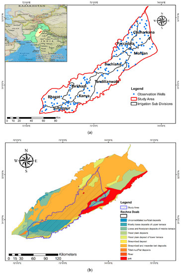
Figure 1.
(a) The geographic location of the study area, representing observation wells and irrigation sub-divisions; (b) The geological map of the study area, representing the geological features.
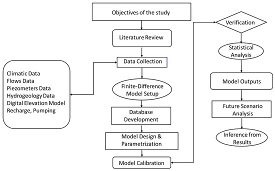
Figure 2.
Flow Chart of the processes involved in the study.
2.2. Data Acquisition
The depth to groundwater-level data (2005–2015) for two periods, i.e., pre-monsoon (June) and post-monsoon (October), were obtained from the Land Reclamation wing of the Punjab Irrigation Department, Faisalabad. The total number of observation wells installed in LCC-E is 213, of which 150 wells’ data were processed for further use.
2.3. Model Development Section
MODFLOW-2005 was used as a model code, with Visual MODFLOW Flex as a graphical user interface, as developed by Waterloo Hydrogeologic. Multiple model scenarios, grid indiscretions, and several hydrogeologic interpretations of the conceptual model can be visualized side by side due to the flexible design of VMOD-Flex. Effective system analysis can be comprehended by converting complex real-world problems into a simple conceptual model approach [46].
The sequential steps in building the conceptual model are listed below:
2.3.1. Defining Modelling Objectives
The model has some pre-defined modelling objective interfaces to define the initial settings. The model requires an initial starting date for the simulation process, and it is imperative to choose relevant start data, depending on the observed field head and pumping data. Therefore, January 2005 was selected as the simulation start date.
2.3.2. Collection of Data Objects
The data objects were collected to define the model area and formulate a conceptual framework. The objects could be imported into the model in three ways: by creating polygons, by creating polylines, or by digitizing within the model interface. The point data objects could also be utilized to generate surface files. For this study, the data objects were prepared in ArcGIS 10.5. A polygon object represented the model surface area, while polylines were used to portray river and canal boundaries.
2.3.3. Layer Development
The layers were developed to discretize the model domain vertically. The bore logs’ point data were utilized to create model layers. The SRTM (Shuttle Radar Topography Mission) data of NASA (National Aeronautics and Space Administration) were used to develop the ground surface elevation by utilizing a 30 m resolution digital elevation model (DEM), whereas the lithological data of the WAPDA (Water and Power Development Authority) were used to divide the model into three vertical layers, with each being 50 m and 70 m thick. The surface maps were produced using Surfer by employing the Kriging technique, with a scale of 1 as the linear variogram model.
2.3.4. Model Structure
To define the structure of the model, the layers were converted into different horizons and named the first, second, and third horizons. The erosional surface was designated to the ground surface, whereas the conformable was designated to the second layer, and the base surface to the third layer, as depicted in Figure 3.
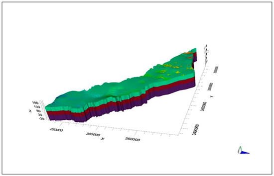
Figure 3.
Model structure zones representing the layers in the Visual MODFLOW Flex environment.
2.4. Hydrogeological Properties
Geologic formations with similar hydrogeologic properties were used to represent hydrostratigraphic units. For this purpose, the data of the WASID (Water and Soil Investigation Department) were utilized from different bore logs [47]. The assumed values for different hydraulic parameters used for the derivation of initial values according to the material of the layers, such as hydraulic conductivity K, specific storage Ss, and specific yield Sy, are given in Table 1. The relevant literature also was used to obtain some soil data, topographical data, and miscellaneous information.

Table 1.
Hydraulic property values used for different lithological units (adapted from [48]).
2.4.1. Derivation of the Horizontal Hydraulic Conductivity (Kh)
The spatially distributed initial values of Kh for different model layers were derived from bore log data. The bore log data provided the depths of varying soil materials, e.g., clay, silt, sand, gravel, etc., that have their specific Kh values. This value was multiplied by the depth of that material to obtain the transmissivity value for that layer. These transmissivity values were added to obtain the total Kh, which was further divided by the total depth of the layer to obtain an average value of Kh as shown by Equation (1):
2.4.2. Derivation of the Vertical Hydraulic Conductivity (Kv)
Similarly, the initial values of Kv for different layers were computed. The Kv value for any individual soil material was taken as 10% of the Kh values based on the literature review. The summation of the depth of all materials was divided by the reciprocal sum of these values multiplied by the layer’s total depth. This gives the mean value of Kv as depicted in Equation (2):
2.5. Initial Hydraulic Head
The depth to water table data were utilized to compute the initial head value. This was achieved by subtracting depth values from the elevation data of any measurement point obtained through DEM. The initial head values were computed from the (2006) data set.
2.6. Boundary Conditions
The constant head boundary condition, also termed “Dirichlet”, or the first-type boundary condition, was used for the link canals. The QB (Qadirabad-Balloki) and TS (Trimmu-Sidhnai) Link Canals were assigned the respective head boundary conditions depending on their historical water level records [38]. Some northern and southern parts of the study area that were not in physical contact with the river were designated as the second type, i.e., the Newman boundary condition. However, pumping from the system was represented by a specified flux boundary.
2.7. Spatial Discretization
To select an appropriate grid due to the model’s regional scale, a grid size of 1000 m × 1000 m was assigned to the model, resulting in 174 columns and 169 rows. The three layers of the model domain were discretized, with the topmost layer as unconfined and the bottom two with adjustable unconfined/confined, having variable storativity and transmissivity values. The layer’s top and bottom followed the horizon elevations due to the deformed grid approach.
2.8. Defining Observation Wells
The observation wells were assigned using an intuitive way of importing well data into VMOD Flex using post-monsoon (2006) heads data. The wells’ data were introduced by linking them with an Excel sheet.
2.9. Transient Model Development (Time-Variant Data)
The transient model was developed after the steady-state model’s calibration by utilizing a time-variant data set. The model was assigned with different time-variant data sets, e.g., recharge, pumping, and observation wells. A schedule was defined by switching steady-state boundary conditions into the transient state. In addition, two stress periods, i.e., Kharif (Summer) and Rabi (Winter), having 182 and 183 days, respectively, along with monthly time steps, were introduced for this simulation.
2.9.1. Derivation of Specific Yield (Sy)
The specific yield values were also computed from the lithological data of the bore logs for the unconfined aquifer system. The respective value of the specific yield for a soil material available in the literature was multiplied by the depth of the material. The values for each layer were summed and divided by the depth of the corresponding layer. That gave the average value of the specific yield for the layers. The relationship is given by Equation (3):
2.9.2. Recharge
To simulate the flux values, a recharge package was used. These values were specified in length/time units and distributed over the top of the entire model. The built-in recharge package multiplied the flux values with the lateral area of each cell to convert them into volumetric flux rates. The values of net recharge were imported into the model for (2006–2013), as adopted from [49]. The net recharge was calculated by subtracting the inflows from the system (seepage from surface water bodies, infiltration, field percolation, etc.) from the system’s outflows (pumping, evapotranspiration, etc.).
2.10. Model Calibration and Validation
The measured or observed wells data were used from 2006–2013 for the calibration and validation of the transient flow model. Data from 2006–2010 was used for calibration and that from 2011–2013 for verification. The steady-state calibration of the model was performed manually for (2006), whereas the transient (dynamic) calibration was carried out for the years 2006–2010 utilizing the PEST code. Several repeated runs of K values and boundary conditions were performed to match simulated and observed values closely. Following the calibration of the model, it was validated with a new data set from (2011–2013) that was not used previously during the calibration process. For this study, the data from 36 observation wells were used, comprising 4 wells from each subdivision.
2.11. Statistical Analysis
Statistical measures evaluated the performance of the model. The study included the root mean square error (RMSE), the normalized root mean square error (NRMSE), the standard error of estimate (SEE), the mean absolute error (MAE), the correlation coefficient, the Nash–Sutcliffe efficiency (NSE), and the coefficient of determination (R2). Most commonly, these are the indices used for the performance evaluation of any model, as indicated in Table 1 [50,51].
2.11.1. Root Mean Square Error
The RMSE shows how closely the model envisages the measured values [52]. The lesser values of that error indicated better prediction.
The RMSE describes the estimation variability. If its value exceeds 1, the model underestimates the prediction variability. If its value is less than 1, there are chances of overestimating the prediction variability [53].
2.11.2. Normalized Root Mean Square Error
The normalized root mean square error is obtained by dividing the RMSE values by the range of maximum and minimum values.
Its value is typically represented as a percentage, and a lesser value indicates lower residual variance [52].
2.11.3. Standard Error of Estimate
The standard error of estimate is usually stated as the calibration residual.
The smaller the standard error of estimate, the more accurate the prediction is [54].
2.11.4. Correlation Coefficient
The statistical measure used to determine the strength of the relationship between two variables is called a correlation coefficient (R). Its value ranges between −1 and +1. The stronger the relationship is, the more positive is the value, and vice versa. A value of more than 1 or less than 1 indicates an error in the measurement [52].
2.11.5. Mean Absolute Error
The mean absolute error is used to describe a model’s forecast accuracy. It indicates the magnitude of an error on averaged forecast values.
The minimum is the value of the MAE; the more accurate are the forecasted values.
2.11.6. Nash–Sutcliffe Efficiency
The best fit of observed vs. modelled values with the (1:1) line is represented by the Nash–Sutcliffe efficiency. The NSE is used extensively for the estimation of the calibrated and validated efficiency of the model [55].
The higher the efficiency, the more accurate the modelled values
2.11.7. Coefficient of Determination
The coefficient of determination describes how well the observed values and modelled values fit with each other. R2 values are determined by taking the square of the correlation coefficient (R).
Its value ranges between (0–1); the larger R2 value indicates the best model fit [55].
2.12. Future Scenario Analysis
Multiple future scenarios were developed to observe the aquifer system’s response to altered pumping and recharge rates. Data from May 2013 were used as the initial conditions. During the entire simulation period (2013–2033), the aquifer hydrogeological characteristics were assumed to be the same.
2.12.1. Scenario I: Business as Usual
Under the business-as-usual scenario, it was assumed that all the conditions of recharge and pumping would remain unchanged from the initial simulation date, and the hydrodynamics of the aquifer system were observed until 2033.
2.12.2. Scenario II: Increased Groundwater Pumping Following the Historical Trend
In Scenario II, the recharge rate to the aquifer system was kept unchanged, or the same as that of Scenario I, whereas the pumping rate was allowed to increase at the tubewell growth rate of 6.91% per annum [56].
2.12.3. Scenario III: Spatially Adjusted Surface Water Supplies and Pumping Pattern
Considering the study area’s recharge and pumping patterns, a new water management scenario was developed. The recharge from irrigation water in the upper parts of the study area was shifted to the lower regions, thereby decreasing the pumping rate at the lower sites. The study area is comprised of nine subdivisions. The upper part of the study area consists of four subdivisions, i.e., CKN (Chuharkana), MHL (Mohlan), PDL (Paccadala) and BCH (Buchiana), whereas the lower part includes the TDW (Tandlianwala), TKH (Tarkhani), KNY (Kanya), BGT (Bhagat), and SPR (Sultanpur) subdivisions. The recharge rate in the upper subdivisions was reduced by 30%, and it was increased by 30% in the lower portions; conversely, the pumping was increased by 30% in the upper part and reduced by 30% in the lower subdivisions.
3. Results and Discussion
3.1. Steady-State Model Calibration
The steady-state model was calibrated manually during the first phase, and groundwater head values (pre-monsoon) for 2006 were used for this purpose. The scatter plot representing measured and modelled head values for the year 2006 is given in Figure 4. The hydraulic conductivity values of the upper and lower aquifers were varied repeatedly so that the difference between the observed and simulated head values would be minimized. The process was continued so that the root mean square error (RMSE) would be kept below 5 m. The value of the correlation coefficient was observed as being 0.98 for the steady-state calibrations, which helps the modeller to understand the model system better; resultantly, the model failure chances were reduced [57]. The manual calibration process is not easy and consumes a lot of time. Still, it helps to minimize the convergence time in the automated calibration process, and it also allows the modeller to understand the model system better, and resultantly, the model failure chances are reduced [58].
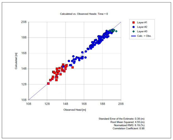
Figure 4.
Scattergram of measured vs. modelled head for the year 2006 (steady state).
3.2. Transient-State Model Calibration
The transient (dynamic) calibration was carried out for the years 2006–2010. The contour and scatter plots for 2006 and 2010 are shown in Figure 5 and Figure 6. Both hydraulic conductivity and specific yield were the adjustable parameters during the transient calibration. The automated estimation tool PEST was run in estimation mode, and parameter values were adjusted during the PEST operation process. The statistical indicators for both the steady state and transient states showed satisfactory results. In the case of the transient model, the SEE and RMSE varied between 0.15–0.18 m and 1.84–2.2 m, with correlation coefficients of 0.98–0.99, respectively.
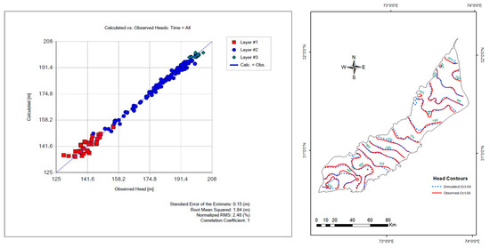
Figure 5.
Observed and simulated scattergram and water level contour plot for October 2006.
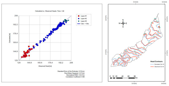
Figure 6.
Observed and simulated scattergram and water level contour plot for October 2010.
3.3. Model Validation
The model was validated with the data from 2011–2013. The data obtained from the model simulation and observation wells showed a satisfactory correlation, and goodness-of-fit was achieved. Figure 7 shows the observed and simulated head contours and scatter plot for 2013. The validation of the model results for 2011–2013 showed that the model performed reasonably well, as the SEE and RMSE were 0.32 and 2.3 m, whereas the correlation coefficient was 1 (Table 2 and Table 3). Overall, the model performance was satisfactory as most of the points lay close to the 1:1 line, with some points showing variations that may be due to the initial parameters’ setting values, or the boundary conditions of the river and link canals may be the potential cause of this drift. Nevertheless, the model showed reasonable results overall for its adoption for future simulation processes.
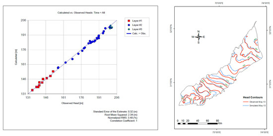
Figure 7.
Observed and simulated scattergram and water level contour plot for May 2013.
Table 2.
Statistical Analysis of Models’ observed and simulated values.
Table 3.
Descriptive Statistical Analysis of increase/decrease in groundwater levels (m) for different future scenarios.
3.4. Results of Future Scenario I
The future groundwater level projections under Scenario I are represented in Figure 8 and Table 4. The hydrographs of each irrigation subdivision reveal overall groundwater level trends up to the year 2033. Due to this scenario, the imbalance between pumping and recharge depicted mixed drawdown levels. The general trend in the upper parts of the study area, particularly in the Buchiana, Mohlan, and Paccadala subdivisions, was a net gain in water levels; however, in the lower subdivisions, i.e., Tarkhani, Tandlianwala, Kanya, Bhagat, and Sultanpur, a lowering of water levels was projected.
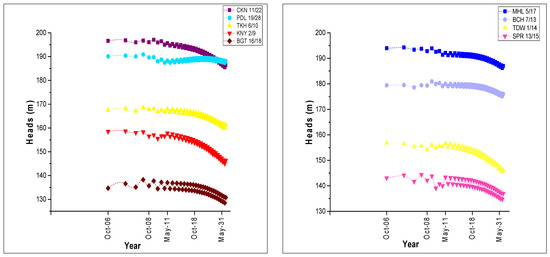
Figure 8.
Predicted groundwater levels for the selected observation wells (Scenario I).
Table 4.
Predicted groundwater level differences for the years 2013–2033 (Scenario I).
Under the business-as-usual scenario, three kinds of future trends are anticipated in the study area, i.e., a gain in water levels, a lowering in water levels, and slight or no-change trends for the two-decade simulation period up to the year 2033, as depicted in Table 4. Four subdivisions showed a lowering of water levels, with a maximum decline of 5.17 m forecast in the Kanya subdivision, represented by the KNY-2/9 observation well, followed by 3.9 m in the Tandlianwala subdivision, TDW-1/14; 3.18 m in the Chuharkana subdivision, CKN-11/22; and 1.43 m of the Tarkhani subdivision, TKH-6/10, whereas three out of nine subdivisions showed a rise in water levels, the maximum was 5 m for the Pacadala subdivision, PDL-19/28; 0.8 m for Buchiana, BCH-7/13; and 0.71 m for Mohlan, MHL-5/17, observation wells. The remaining two subdivisions, Sultanpur and Bhagat, had a slight change in water levels, i.e., 0.4 and 0.1 m, represented by the SPR-13/15 and BGT-16/18 observation wells.
The water level contour maps (Figure 9) describe the spatial pattern of the water levels of the whole study area, with 5-year time intervals for a better understanding and visualization of the years 2018, 2023, 2028, and 2033. The contour intervals were kept constant for each year. The maximum and minimum contour lines ranged between 198–135 and 190–128 m for 2018–2033. The variation in contour lines indicates the variation in water levels spatially and temporally, following the results tabulated above. The shifting of the contour value suggests an imbalance between recharge and pumping. The upper parts of the study area exhibited an upward trend in contour values under the business-as-usual scenario, which may be due to more recharge as compared with pumping, whereas the middle and lower-middle parts exhibited a lowering of the water level contours, indicating excessive pumping and reduced recharge. In the regions where an improvement in water levels is observed, the seepage from the irrigation system seems to be intensive compared to the discharge through pumping wells [18]. There is not much noticeable change at the study area’s tail end, which shows a balance between recharge and pumping. Similar results are reported by [48,59] in their studies in other regions of Rechna Doab, Pakistan. The reduction in groundwater levels was more prominent in non-canal command areas in irrigated areas of Punjab, as reported by Qureshi, et al. [60], and the evident reason was that, in noncanal command areas, recharge was less, and reliance on groundwater was more to fulfil the requirements of crops [61]. Other than the overexploitation of groundwater, reduction in canal command areas which result in less natural recharge of the aquifer, and erratic rainfall patterns are other potential causes of declining water levels [18]. The decline in water levels also impacts water quality, and an increase in water salinity is observed [48,62]. The reason behind increasing the groundwater salinity with increased pumping is that, in the whole Indus Basin, the deeper aquifers are of a marine nature [63], thereby resulting in deteriorated groundwater quality at deeper depths, whereas the shallow water in the aquifer is of good quality due to recharge from different sources [62].
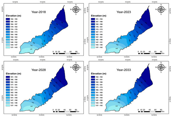
Figure 9.
Water level contour maps for Scenario I for the years 2018–2033.
3.5. Scenario II (Historical Trend of Pumping)
The projected scenario results with increased pumping following historical trends in the study area are represented in Figure 10 and Table 5. The complete study area observed an overall decline in water levels, indicating a clear imbalance between recharge and pumping. The hydrographs identified that the upper part of the study area would have comparatively less of a decline in the water level, whereas the middle and the lower part were anticipated to have maximum drawdown.
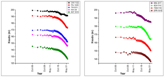
Figure 10.
Predicted groundwater levels for the selected observation wells (Scenario II).
Table 5.
Predicted groundwater level differences for the years 2013–2033 (Scenario II).
Table 5 summarizes the temporal change in groundwater levels in each subdivision. In almost every subdivision, a declining trend in water level was observed. The drop in water levels could also be categorized into three categories, i.e., up to 5 m (normal), 5–10 m (moderate), and >10 m (high). The CKN-11/22 observation well only fell into the minimum category, with a 6.03 m drop in water level; similarly, only one observation well, MHL-5/17, fell into the moderate category, with a 9.97 m drawdown. All of the other wells fell into the high category of dropdowns. The maximum drawdown was anticipated in the BGT-16/18 observation well, which showed a 15.68 m decline, followed by the PDL-19/28, TKH-6/10, BCH-7/13, KNY-2/9, TDW-1/14, and SPR-13/15 wells having 15.04, 14.67, 14.5, 14.29, 12.4, and 11.23 m drawdown, respectively.
The spatial pattern of water levels in the complete study area is depicted through contour maps (Figure 11). The maps were drawn with a 5-year interval representing the years 2018, 2023, 2028, and 2033, respectively. A substantial shift in contour lines indicated a sizeable drawdown in the research area. The upper parts of the study area exhibited the lower drawdown due to more recharge through the water bodies, whereas the middle and lower portion was anticipated to have maximum drawdown under this future scenario. The drastic drop in water levels indicated a disparity between recharge and pumping. Lowering the water level in the study area could cause severe threats in the near future as the aquifer would be depleted at a rapid pace, ultimately increasing the pumping costs. A study by [64] in the Indus Basin, Pakistan, concluded that lowering the water table could substantially affect the pumping price. Deep electric power-driven tube wells (>20 m) could cost up to USD 5000 in comparison with shallow tube wells (<6 m), which cost up to USD 1000. Similarly, the pumping cost of deep tube wells was also more, i.e., USD 8.61 per acre inch, compared to USD 18.78 for 31 and 91 m lifts of water [65]. It was observed that groundwater pumping costs per cubic meter could increase about 3.5 times in the case of water levels dropping from 6 to 21 m [56].
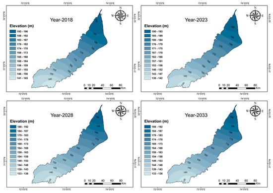
Figure 11.
Water level contours for Scenario II for the years 2018–2033.
3.6. Scenario III (Spatially Adjusted Irrigation Recharge and Pumping)
The piezometric water levels for the spatially adjusted recharge and discharge patterns were worked out by the model up to the year 2033 and are depicted in Figure 12 and Table 6. The analysis of the hydrographs revealed an overall decline in water levels in the upper four subdivisions, where irrigation recharge was reduced to 30% and pumping was allowed to increase by 30%. Overall recovery in the water levels was observed in the lower five subdivisions of the study area, where irrigation recharge was allowed to increase by 30%, and consequently, pumping was decreased by 30%. Due to increased recharge and a decline in pumping, a new equilibrium in the water levels was observed in the lower parts.
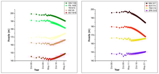
Figure 12.
Predicted groundwater levels for the selected observation wells (Scenario III).
Table 6.
Predicted groundwater level differences for the years 2013–2033.
Under the spatially adjusted canal water supply and pumping scheme, two kinds of future water level change trends were observed in the study area. The upper four sub-divisions showed a lowering of water levels; a maximum drawdown of 10.7 m was observed in Buchiana BCH-7/13, followed by 10.6, 6.93, and 6.58 m for the Mohlan, MHL-5/17; Chuharkana, CKN-11/22; and Paccadala, PDL-19/28, observation wells. The remaining five subdivisions, which represented the study area’s lower portion, established a new equilibrium in the water levels, and recovery in water levels was observed. Maximum recovery or rise in water levels was observed in the Tarkhani and Bhagat subdivisions, which showed an overall increase of 7.99 and 6.87 m, respectively. The Kanya, Tandlianwala, and Sultanpur subdivisions also showed an increase in water levels with a 5.86, 2.93 and 2.24 m increase.
The 5-year interval contour maps (Figure 13) for the simulation periods of 2018, 2023, 2028, and 2033 depicted spatial and temporal variations in the water levels. The upper parts of the study area exhibited a downward trend in the contour values under the spatially adjusted recharge and pumping scenarios due to decreased recharge and increased pumping; on the contrary, the lower-middle parts exhibited a rise in water level contours, indicating reduced pumping and an increase in irrigation recharge. The results are in accordance with a study by [40] in Rechna Doab and by [62] for the LCC-W region. The results revealed that, if surface water supplies are shifted from the upper parts of the study area towards the lower parts, and similarly, the groundwater pumpage pattern can also be altered, this will not only reduce the groundwater level depletion but also help to minimize the groundwater salinity and waterlogging problems in the area as well [48].
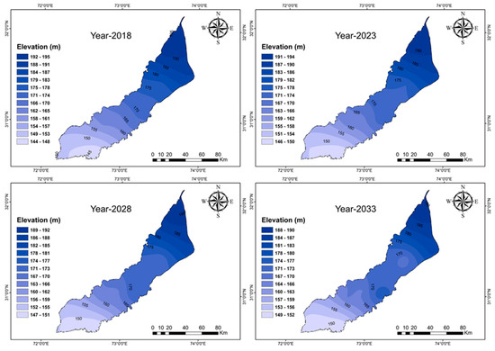
Figure 13.
Water level contours for Scenario III for the years 2018–2033.
4. Conclusions and Recommendations
The following conclusions were drawn from the research work:
- •
- Due to its importance from the agricultural perspective, the Lower Chenab Canal Command Area is vital and contributes a lot to the country’s gross domestic product.
- •
- The area’s aquifer is highly stressed and requires immediate attention in regard to recharge and pumping patterns.
- •
- A future-scenario-based, three-layer groundwater flow model was developed, which gave satisfactory results regarding aquifer storage and releases.
- •
- Calibration of the model using 160 observations of groundwater levels gives a relatively good fit with a SEE of 0.15–0.18 m and a RMSE of 1.8–2.2 m.
- •
- The future scenario results under the business-as-usual scenario revealed that there was a net gain of water levels in the upper parts of the study area with a maximum increase of 5 m, whereas a lowering of water levels was predicted in the central and lower parts, with a maximum drop of 5.17 m.
- •
- For Scenario II, which followed the historical trend of pumping in the complete LCC-E, an overall decline in water levels was observed, with a minimum decline of 6.03 m and a maximum decline of 15.68 m.
- •
- The water levels for the spatially adjusted recharge and discharge patterns under the future management Scenario III gave new water dynamics with a maximum drawdown of 10.7 m and a maximum recovery of 7.99 m in water levels.
Our recommendations include:
- •
- Utilizing the underlying unconfined aquifer of the study area as a water storage reservoir as it has an enormous potential to store water, especially during the high flow season of the river and the monsoon period. The shallow aquifer must be recharged artificially.
- •
- Reallocating the surface water supplies to avoid waterlogging in the upper parts of the LCC and lower water levels in the lower portions. This can be achieved by shifting 30% of canal water supplies from the upper to the lower regions. This reduction in supplies for the upper parts could be compensated by additional pumping, whereas the lower parts would be able to reduce pumping in the same proportion as receiving more canal supplies. This would allow the water levels to recover in the study area.
- •
- The artificial recharging of the aquifer through flood-water spreading and ponding through rainwater harvesting in the depressions can be very effective in highly stressed areas.
- •
- Implementing proper pumping and groundwater management policy legislation in the study area to sustainably safeguard precious groundwater resources.
5. Limitations of the Study
A three-layered hydrogeological MODFLOW-based model can provide good results for future groundwater level simulations. Yet, there are some limitations which should not be overlooked while developing any prospective modelling study. For instance, the observation wells’ data quantity and quality play a pivotal role in the future forecasting of groundwater levels. The scarce piezometer network and their density could be increased, and data quality should be improved with automatic data loggers to obtain better prediction results.
Author Contributions
Conceptualization, M.A. (Muhammad Awais); Methodology, A.N.; Soft-ware, M.A. (Muhammad Awais); Validation, R.A.; Formal analysis, M.A. (Muhammad Awais); Investi-gation, M.A. (Muhammad Awais); Resources, M.A. (Muhammad Arshad); Data curation, M.A. (Muhammad Awais) and M.M.W.; Writing—original draft, M.A. (Muhammad Awais); Writing—review & editing, M.M.W., A.S. and M.R.; Visualization, J.N.C., Q.M. and M.A. (Matlob Ahmad); Supervision, M.A. (Muhammad Arshad); Project administration, S.R.A.; Funding acquisition, A.N. All authors have read and agreed to the published version of the manuscript.
Funding
This research was funded by Higher Education Commission of Pakistan under the project (NRPU Project-No 4587) and the APC was funded by TU Delft.
Institutional Review Board Statement
Not applicable.
Informed Consent Statement
Not applicable.
Data Availability Statement
The data in figures and tables used to support the findings of the study are included herein.
Acknowledgments
The authors are grateful to the Higher Education Commission (HEC) of Pakistan for funding the research under NRPU Project-No 4587. We are also thankful to the Land Reclamation wing of the Irrigation Department of the Government of Punjab, WAPDA, and PMD for providing the secondary data for research.
Conflicts of Interest
On behalf of all of the authors, the corresponding author states that there are no conflict of interest.
References
- Barlow, M.; Clarke, T. Blue Gold: The Battle against Corporate Theft of the World’s Water; Routledge: London, UK, 2017. [Google Scholar]
- Bogardi, J.J.; Bharati, L.; Foster, S.; Dhaubanjar, S. Water and its management: Dependence, linkages and challenges. In Handbook of Water Resources Management: Discourses, Concepts and Examples; Springer: Berlin/Heidelberg, Germany, 2021; pp. 41–85. [Google Scholar]
- Benz, S.A.; Bayer, P.; Blum, P. Global patterns of shallow groundwater temperatures. Environ. Res. Lett. 2017, 12, 034005. [Google Scholar] [CrossRef]
- Gleeson, T.; Wada, Y.; Bierkens, M.F.; van Beek, L.P. Water balance of global aquifers revealed by groundwater footprint. Nature 2012, 488, 197. [Google Scholar] [CrossRef] [PubMed]
- Qadir, M.; Boers, T.M.; Schubert, S.; Ghafoor, A.; Murtaza, G. Agricultural water management in water-starved countries: Challenges and opportunities. Agric. Water Manag. 2003, 62, 165–185. [Google Scholar] [CrossRef]
- Sun, H.; Zhang, X.; Wang, E.; Chen, S.; Shao, L. Quantifying the impact of irrigation on groundwater reserve and crop production–A case study in the North China Plain. Eur. J. Agron. 2015, 70, 48–56. [Google Scholar] [CrossRef]
- Mirzaei, A.; Saghafian, B.; Mirchi, A.; Madani, K. The groundwater-energy-food nexus in Iran’s agricultural sector: Implications for water security. Water 2019, 11, 1835. [Google Scholar] [CrossRef]
- Shah, T. The groundwater economy of South Asia: An assessment of size, significance and socio-ecological impacts. In The Agricultural Groundwater Revolution: Opportunities and Threats to Development; CAB International: Oxford, UK, 2007; pp. 7–36. [Google Scholar]
- Choudhary, M.R. Optimal Conjunctive Use of Surface and Groundwater in a Watercourse Command Area of the Indus Basin. Ph.D. Thesis, Colorado State University, Fort Collins, CO, USA, 1989. [Google Scholar]
- Muzammil, M.; Zahid, A.; Breuer, L. Water Resources Management Strategies for Irrigated Agriculture in the Indus Basin of Pakistan. Water 2020, 12, 1429. [Google Scholar] [CrossRef]
- Qureshi, A.S. Groundwater Governance in Pakistan: From Colossal Development to Neglected Management. Water 2020, 12, 3017. [Google Scholar] [CrossRef]
- Bakhsh, A.; Awan, Q. Water issues in Pakistan and their remedies. In Proceedings of the National Symposium on Drought and Water Resources, Lahore, Pakistan, 16 March 2002; pp. 145–150. [Google Scholar]
- MoWP. Handbook on Water Crisis of Pakistan; Ministry of Water and Power: Islamabad, Pakistan, 2012.
- Ashraf, A.; Ahmad, Z.; Akhter, G. Monitoring groundwater flow dynamics and vulnerability to climate change in Chaj Doab, Indus Basin, through modeling approach. In Groundwater of South Asia; Springer: Berlin/Heidelberg, Germany, 2018; pp. 593–611. [Google Scholar]
- Qureshi, A.S. Water management in the Indus basin in Pakistan: Challenges and opportunities. Mt. Res. Dev. 2011, 31, 252–260. [Google Scholar] [CrossRef]
- MacDonald, A.; Bonsor, H.; Ahmed, K.; Burgess, W.; Basharat, M.; Calow, R.; Dixit, A.; Foster, S.; Gopal, K.; Lapworth, D. Groundwater quality and depletion in the Indo-Gangetic Basin mapped from in situ observations. Nat. Geosci. 2016, 9, 762–766. [Google Scholar] [CrossRef]
- Jabeen, M.; Ahmad, Z.; Ashraf, A. Predicting behaviour of the Indus basin aquifer susceptible to degraded environment in the Punjab province, Pakistan. Model. Earth Syst. Environ. 2020, 6, 1633–1644. [Google Scholar] [CrossRef]
- Khan, A.; Iqbal, N.; Ashraf, M.; Sheikh, A.A. Groundwater Investigations and Mapping in the Upper Indus Plain; Pakistan Council of Research in Water Resources (PCRWR): Islamabad, Pakistan, 2016. [Google Scholar]
- Ashraf, A.; Ahmad, Z. Regional groundwater flow modelling of Upper Chaj Doab of Indus Basin, Pakistan using finite element model (Feflow) and geoinformatics. Geophys. J. Int. 2008, 173, 17–24. [Google Scholar] [CrossRef]
- Bhutta, M.N.; Smedema, L.K. One hundred years of waterlogging and salinity control in the Indus valley, Pakistan: A historical review. Irrig. Drain. 2007, 56, S81–S90. [Google Scholar] [CrossRef]
- Gómez, C.; Green, D.R. Small unmanned airborne systems to support oil and gas pipeline monitoring and mapping. Arab. J. Geosci. 2017, 10, 1–17. [Google Scholar] [CrossRef]
- PBOS. Agriculture Statistics of Pakistan; Statistics Division, Government of Pakistan: Islamabad, Pakistan, 2010–2011.
- Shahab, A.; Shihua, Q.; Rashid, A.; Hasan, F.U.; Sohail, M.T. Evaluation of Water Quality for Drinking and Agricultural Suitability in the Lower Indus Plain in Sindh Province, Pakistan. Pol. J. Environ. Stud. 2016, 25, 2563–2574. [Google Scholar] [CrossRef] [PubMed]
- Bhatti, M.T.; Anwar, A.A.; Aslam, M. Groundwater monitoring and management: Status and options in Pakistan. Comput. Electron. Agric. 2017, 135, 143–153. [Google Scholar] [CrossRef]
- Zulfiqar, F.; Thapa, G.B. Agricultural sustainability assessment at provincial level in Pakistan. Land Use Policy 2017, 68, 492–502. [Google Scholar] [CrossRef]
- Ahmed, K.; Shahid, S.; Demirel, M.C.; Nawaz, N.; Khan, N. The changing characteristics of groundwater sustainability in Pakistan from 2002 to 2016. Hydrogeol. J. 2019, 27, 2485–2496. [Google Scholar] [CrossRef]
- Van der Wal, M.M.; De Kraker, J.; Kroeze, C.; Kirschner, P.A.; Valkering, P. Can computer models be used for social learning? A serious game in water management. Environ. Model. Softw. 2016, 75, 119–132. [Google Scholar] [CrossRef]
- Basco-Carrera, L.; Warren, A.; van Beek, E.; Jonoski, A.; Giardino, A. Collaborative modelling or participatory modelling? A framework for water resources management. Environ. Model. Softw. 2017, 91, 95–110. [Google Scholar] [CrossRef]
- El Osta, M. Maximizing the management of groundwater resources in the Paris–Abu Bayan reclaimed area, Western Desert, Egypt. Arab. J. Geosci. 2018, 11, 1–20. [Google Scholar]
- Khadri, S.; Pande, C. Ground water flow modeling for calibrating steady state using MODFLOW software: A case study of Mahesh River basin, India. Model. Earth Syst. Environ. 2016, 2, 39. [Google Scholar] [CrossRef]
- Siade, A.; Rathi, B.; Prommer, H.; Welter, D.; Doherty, J. Using heuristic multi-objective optimization for quantifying predictive uncertainty associated with groundwater flow and reactive transport models. J. Hydrol. 2019, 577, 123999. [Google Scholar] [CrossRef]
- Anderson, M.P.; Woessner, W.W.; Hunt, R.J. Applied Groundwater Modeling: Simulation of Flow and Advective Transport; Academic press: Cambridge, MA, USA, 2015. [Google Scholar]
- Masoud, M.H.; Schneider, M.; El Osta, M. Recharge flux to the Nubian Sandstone aquifer and its impact on the present development in southwest Egypt. J. Afr. Earth Sci. 2013, 85, 115–124. [Google Scholar] [CrossRef]
- White, J.T. Forecast first: An argument for groundwater modeling in reverse. Groundwater 2017, 55, 660–664. [Google Scholar] [CrossRef] [PubMed]
- Malenica, L.; Gotovac, H.; Kamber, G.; Simunovic, S.; Allu, S.; Divic, V. Groundwater flow modeling in karst aquifers: Coupling 3d matrix and 1d conduit flow via control volume isogeometric analysis—Experimental verification with a 3D physical model. Water 2018, 10, 1787. [Google Scholar] [CrossRef]
- Basharat, M.; Tariq, A.-U.-R. Command-scale integrated water management in response to spatial climate variability in Lower Bari Doab Canal irrigation system. Water Policy 2014, 16, 374–396. [Google Scholar] [CrossRef]
- Sarwar, A. A Transient Model Approach to Improve on-Farm Irrigation and Drainage in Semi-Arid Zones; International Water Management Institute (IWMI): Lahore, Pakistan, 2000. [Google Scholar]
- Sarwar, A.; Eggers, H. Development of a conjunctive use model to evaluate alternative management options for surface and groundwater resources. Hydrogeol. J. 2006, 14, 1676–1687. [Google Scholar] [CrossRef]
- Mujtaba, G.; Ahmed, Z.; Ophori, D. Management of groundwater resources in Punjab, Pakistan, using a groundwater flow model. J. Environ. Hydrol. 2007, 15, 1–14. [Google Scholar]
- Khan, S.; Rana, T.; Ullah, K.; Christen, E.; Nafees, M. Investigating Conjunctive Water Management Options Using a Dynamic Surface-Groundwater Modelling Approach: A Case Study of Rechna Doab; Report No 35/03; CSIRO: Canberra, Australia, 2003. [Google Scholar]
- Jehangir, W.A.; Qureshi, A.S.; Ali, N. Conjunctive Water Management in the Rechna Doab: An Overview of Resources and Issues; IWMI: Lahore, Pakistan, 2002; Volume 48. [Google Scholar]
- PMD. Climate and Astronomical Data. Available online: http://www.pmd.gov.pk/ (accessed on 10 September 2018).
- Usman, M.; Liedl, R.; Arshad, M.; Conrad, C. 3-D numerical modelling of groundwater flow for scenario-based analysis and management. Water SA 2018, 44, 146–154. [Google Scholar] [CrossRef]
- Khalid, P.; Sanaullah, M.; Sardar, M.J.; Iman, S. Estimating active storage of groundwater quality zones in alluvial deposits of Faisalabad area, Rechna Doab, Pakistan. Arab. J. Geosci. 2019, 12, 1–9. [Google Scholar] [CrossRef]
- Awais, M.; Arshad, M.; Shah, S.H.H.; Anwar-ul-Haq, M. Evaluating groundwater quality for irrigated agriculture: Spatio-temporal investigations using GIS and geostatistics in Punjab, Pakistan. Arab. J. Geosci. 2017, 10, 1–15. [Google Scholar] [CrossRef]
- Anderson, M.P.; Woessner, W.W. Applied Modeling of Groundwater Flow-Simulation of Flow and Advective Transport; Elsevier Science: Amsterdam, The Netherlands, 1992. [Google Scholar]
- Khan, M.A. Hydrogeological Data. Rechna Doab Vol. I; Project Planning Organization, Water and Power Development Authority (WAPDA): Lahore, Pakistan, 1978. [Google Scholar]
- Khan, S.; Rana, T.; Gabriel, H.; Ullah, M.K. Hydrogeologic assessment of escalating groundwater exploitation in the Indus Basin, Pakistan. Hydrogeol. J. 2008, 16, 1635–1654. [Google Scholar] [CrossRef]
- Usman, M.; Liedl, R.; Kavousi, A. Estimation of distributed seasonal net recharge by modern satellite data in irrigated agricultural regions of Pakistan. Environ. Earth Sci. 2015, 74, 1463–1486. [Google Scholar] [CrossRef]
- Saatsaz, M.; Chitsazan, M.; Eslamian, S.; Sulaiman, W.N.A. The application of groundwater modelling to simulate the behaviour of groundwater resources in the Ramhormooz Aquifer, Iran. Int. J. Water 2011, 6, 29–42. [Google Scholar] [CrossRef]
- Moriasi, D.N.; Arnold, J.G.; Van Liew, M.W.; Bingner, R.L.; Harmel, R.D.; Veith, T.L. Model evaluation guidelines for systematic quantification of accuracy in watershed simulations. Trans. ASABE 2007, 50, 885–900. [Google Scholar] [CrossRef]
- Delgado, C.; Pacheco, J.; Cabrera, A.; Batllori, E.; Orellana, R.; Bautista, F. Quality of groundwater for irrigation in tropical karst environment: The case of Yucatan, Mexico. Agric. Water Manag. 2010, 97, 1423–1433. [Google Scholar] [CrossRef]
- ESRI. Arc GIS Desktop, Documentation. Available online: http://desktop.arcgis.com/en/documentation/ (accessed on 1 April 2019).
- Cocci, M.D.; Plagborg-Møller, M. Standard Errors for Calibrated Parameters; Princeton University: Princeton, NJ, USA, 2019. [Google Scholar]
- Ouyang, F.; Zhu, Y.; Fu, G.; Lü, H.; Zhang, A.; Yu, Z.; Chen, X. Impacts of climate change under CMIP5 RCP scenarios on streamflow in the Huangnizhuang catchment. Stoch. Environ. Res. Risk Assess. 2015, 29, 1781–1795. [Google Scholar] [CrossRef]
- Basharat, M.; Hashmi, D. Groundwater management and recharge potential as an alternate to mega surface storages. Commun. Water Qual. Chall. Oppor. World Water Day March 2010, 114–131. Available online: https://www.researchgate.net/publication/291994461_Groundwater_management_and_recharge_potential_as_an_alternate_to_mega_surface_storages (accessed on 1 April 2019).
- Chakraborty, S.; Maity, P.K.; Das, S. Investigation, simulation, identification and prediction of groundwater levels in coastal areas of Purba Midnapur, India, using MODFLOW. Environ. Dev. Sustain. 2020, 22, 3805–3837. [Google Scholar] [CrossRef]
- Usman, M.; Reimann, T.; Liedl, R.; Abbas, A.; Conrad, C.; Saleem, S. Inverse parametrization of a regional groundwater flow model with the aid of modelling and GIS: Test and application of different approaches. ISPRS Int. J. Geo Inf. 2018, 7, 22. [Google Scholar] [CrossRef]
- Shakoor, A.; Arshad, M.; Ahmad, R.; Khan, Z.M.; Qamar, U.; Farid, H.U.; Sultan, M.; Ahmad, F. Development of groundwater flow model (MODFLOW) to simulate the escalating groundwater pumping in the Punjab, Pakistan. Pak. J. Agric. Sci. 2018, 55, 629–638. [Google Scholar]
- Qureshi, A.S.; McCornick, P.G.; Qadir, M.; Aslam, Z. Managing salinity and waterlogging in the Indus Basin of Pakistan. Agric. Water Manag. 2008, 95, 1–10. [Google Scholar] [CrossRef]
- Usman, M.; Abbas, A.; Saqib, Z.A. Conjunctive use of water and its management for enhanced productivity of major crops across tertiary canal irrigation system of Indus Basin in Pakistan. Pak. J. Agric. Sci. 2016, 53, 257–264. [Google Scholar]
- Shakoor, A. Hydrogeologic Assessment of Spatio-Temporal Variation in Groundwater Quality and Its Impact on Agricultural Productivity; University of Agriculture: Faisalabad, Pakistan, 2015. [Google Scholar]
- Saeed, M.; Asghar, M.; Bruen, M. Options for skimming fresh groundwater in the Indus Basin of Pakistan: A review. J. Groundw. Hydrol. 2003, 45, 259–278. [Google Scholar] [CrossRef][Green Version]
- Qureshi, A. Groundwater management in Pakistan: The question of balance. Centen. Celebr. Pap. 2012, 717, 207–217. [Google Scholar]
- Dumler, T.J.; Rogers, D.H.; O’Brien, D.M. Irrigation Capital Requirements and Energy Costs; Agricultural Experiment Station and Cooperative Extension Service, Kansas State University: Manhattan, KS, USA, 2007. [Google Scholar]


Disclaimer/Publisher’s Note: The statements, opinions and data contained in all publications are solely those of the individual author(s) and contributor(s) and not of MDPI and/or the editor(s). MDPI and/or the editor(s) disclaim responsibility for any injury to people or property resulting from any ideas, methods, instructions or products referred to in the content. |
© 2022 by the authors. Licensee MDPI, Basel, Switzerland. This article is an open access article distributed under the terms and conditions of the Creative Commons Attribution (CC BY) license (https://creativecommons.org/licenses/by/4.0/).