Article

The Impacts of China’s Resident Tourism Subsidy Policy on the Economy and Air Pollution Emissions

1
Laboratory for Earth Surface Processes, College of Urban and Environmental Sciences, Peking University, Beijing 100871, China
2
School of Statistics, University of International Business and Economics, Beijing 100029, China
3
College of Economics and Management, Nanjing University of Aeronautics and Astronautics, Nanjing 210016, China
*
Author to whom correspondence should be addressed.
Sustainability 2023, 15(10), 8351; https://doi.org/10.3390/su15108351
Submission received: 27 February 2023 / Revised: 10 May 2023 / Accepted: 18 May 2023 / Published: 21 May 2023

Abstract

:
Currently, tourism is an important contributor to the Chinese economy. The Chinese government issued Several Opinions of the State Council on Promoting the Reform and Development of Tourism and Several Opinions of the General Office of the State Council on Further Promoting Tourism Investment and Consumption, which are aimed at promoting tourism development. In this study, we use a multiregional and multisectoral computable general equilibrium model (CGE model) to simulate the effects of different levels of resident tourism subsidy policies on the economy and environment in China. Our analysis shows that tourism subsidies are beneficial to economic growth and support the transition to a low-carbon society. In addition, resident tourism subsidy policy has a positive effect on the national emission reduction of CO2, CO, NOX, PM2.5, and SO2. At the regional level, more significant emission reduction potential is present in provinces with more energy consumption and a more developed heavy industry, such as Shandong, Guizhou, and Inner Mongolia. Therefore, this study indicates that resident tourism subsidies can be an effective policy suggestion to promote the transition to a green society and air pollutant emission reduction.

1. Introduction

As a compound industry, tourism is the overall key subindustry of the Chinese tertiary industry. The Chinese government issued Several Opinions of the State Council on Promoting the Reform and Development of Tourism in 2014 and made further proposals in 2015. These opinions aim at reform and innovation to boost tourism investment and consumption, promote the development of the modern service industry, and increase employment. Currently, tourism revenue is an important component of the Chinese economy. According to basic information on the tourism market released by the China Tourism Academy (Data Center of the Ministry of Culture and Tourism), in 2019, the growth rate of the tourism economy remained higher than that of gross domestic product (GDP), with the comprehensive contribution of tourism to GDP being CNY 10.94 trillion, accounting for 11.05% of total GDP. Thereinto, domestic tourism revenue reached CNY 5.73 trillion, up 11.7% from the same period in the previous year. Moreover, the number of people directly and indirectly employed in the tourism industry was reported to be 79.87 million, representing 10.31% of the nation’s total employed population. Tourism development and the environment are interdependent. In the face of global climate change, the China Tourism Administration Opinions on the Response of Tourism to Climate Change (2008) called for full recognition of the importance of tourism in combating climate change. During the 75th United Nations General Assembly, China proposed that carbon dioxide (CO2) emissions should reach a peak before 2030 and that it would strive to achieve carbon neutrality by 2060. The Chinese tourist industry is committed to fighting climate change due to greenhouse gas (GHG) emissions.
Although active responses to climate change and pollution reduction have become a global consensus, the implementation of climate change initiatives has corresponding socioeconomic impacts and affects people employed in specific industries. The phrase “just transition” is frequently used to describe the guidelines and tactics required to lessen the effects on employees as an economy transitions to a sustainable, lower carbon future [1]. In 2015, the Paris Agreement included just transition in its verbiage, emphasizing that corresponding employment issues should be paid close attention when addressing climate change. In recent years, an increasing number of countries have put forward goals and measures related to just transition in their plans concerning climate change issues and energy structure revolution. Some notable studies on just transition in different countries include those of Evans and Phelan [2], Dalglish, Leslie [3], Snell [4], Cock [5], Harrahill and Douglas [6], Cha [7], and Moodie, Tapia [8]. The issue of employment and transition is becoming more mainstream in the process of international climate governance, and achieving a fair and just low-carbon transition is critical to the achievement of climate goals. At the Leaders’ Summit on Climate in 2021, President Xi said that it is necessary to follow the general direction of the modern technological and industrial revolutions, take advantage of the enormous development opportunities brought about by green transformation, and strive to achieve social fairness and justice in the process of green transformation. In light of this, as an important part of energy transition and industrial structure revolution, tourism should contribute to emission reduction and socially just transition in response to current political imperatives.
There is an extensive literature exploring the relationships between and impact of tourism on the economy and emissions. Tourism is a low-carbon industry and the leading industry coping with global climate change, energy savings, and CO2 emission reduction [9]. Wang, Juan [10] found that a long-term cointegration relationship exists between tourism economic growth and carbon emissions, while Chinese tourism economic growth and CO2 emissions have been relatively decoupled in most years. Based on input–output (IO) models, Xiaoyang, Tian [11] pointed out that tourism is strongly correlated with other industries, extending the tourism industry chain to boost China’s sustainable development. In addition, the IO model supports the research that found that tourism plays a positive role in promoting both employment and reemployment [12]. Li et al. balanced tourism’s economic benefit with its CO emissions by using an IO model and tourism satellite accounts [13]. Moreover, studies in other countries, including those in Australia [14], Sweden [15], Spain [16], and Romania [17], also used IO models to analyze the impact of tourism on the economy and emissions. Such a model can systematically quantify the interdependence between various departments in a complex economic system and can measure the economic contribution of tourism in a deep and quantitative way. However, this model assumes a fixed-proportion relationship between the various inputs in the production of one product and is deficient in the function of transforming the factor input in the production process into the demand for goods. Moreover, this model has some limitations in terms of its evaluation application.
Computable general equilibrium (CGE) models are a powerful and widely used method in economic and environmental policy analysis; they are prevailingly used to analyze the effects of economic or emission policies on tourism. Zhou, Yanagida [18] compared the IO and CGE models in terms of the impact of a reduction in visitor expenditure on Hawaii’s economy. The results of the two approaches are similar in magnitude, but a key feature of CGE models is their capacity to take into account intersectoral resource transfers, which accounts for the disparities between the IO and CGE results. Using a global CGE model, Berrittella, Bigano [19] investigated the economic effects of fluctuations in tourism demand brought on by climate change. Dwyer [20] gave a summary of the part CGE modeling has and may play in calculating the economic effects of tourism shocks as well as in the simulation and execution of tourism policies by destination management. Studies from Scotland [21], Spain [22], Australia [23], Singapore [24], Thailand [25], the Philippines [26], and Kenya [27] have also used CGE models to explore the effects of tourism policies on the national economy. In China, Li et al. firstly used CGE modeling to project the economic impact of tourism generated by the Beijing Olympics [28] and discovered that the growth of tourism might lower the outputs of sectors with excess capacity and reallocate surplus labor to industries connected to tourism [29]. In addition, Zhang presented a simulation analysis of the potential impacts of a carbon tax policy on China’s tourist industry’s carbon emissions and economic wellbeing using a CGE model [30] and then investigated the financial effects of the carbon tax on the Chinese tourism industry under two scenarios: a single carbon tax and a carbon tax plus compensation [31]. Subsidizing tourism is also a common tourism-related policy. Schubert and Brida [32] explored the short- and long-term impacts of a production subsidy for a small open economy’s tourist industry. In Singapore, whether subsidizing tourism policy is an effective means to restore the tourism economy has been studied [33]. Moreover, Meng, Pham [34] simulated the short-term impacts on the Chinese tourist sector of an emission trading system (ETS) and two supplementary policies, showing that tourism subsidies could soften the negative impacts of the ETS.
Most of the abovementioned CGE-related studies focus on a single country or region as a whole. However, the tourism industry involves almost all regions and is unbalanced, so it is necessary to discuss its economic and environmental impacts across different regions. Although Li researched the impact of an increase in international tourism reception on 30 provinces, there still remains a lack of research on the economic and environmental impacts of domestic regional tourism.
The remainder of this paper is structured as a multiregion and multisectoral CGE model to analyze the effects of tourism subsidy policies on China’s economy and environment and explore how tourism price subsidies contribute to boosting the regional economy, promoting employment, reducing air pollutant emissions, and supporting the transition to a low-carbon society. Compared with previous studies, this study carried out regional simulation analysis. Trade activities between different regions are reflected in the model, which can better reflect the results of regional interaction. At the same time, different from pure economic analysis, this study combines pollution emission data with economic activity data to extend the role of policy to the field of pollution emission and contributes to the new field of combining the economic effects of tourism with air pollution emissions. Air-quality-related pollutants are selected for their environmental impact, including CO2, carbon monoxide (CO), nitrogen oxide (NOX), particulate matter with a diameter of 2.5 μm or smaller (PM2.5), and sulfur dioxide (SO2). We simulate two different scenarios of tourism subsidy levels relative to the benchmark case (SCA1 scenario) in 2020. The economic constraints under different scenarios are found to lead to changes in the economy and emissions.

2. Methods

2.1. CGE Model

This study develops a multiregional and multisector CGE model for China to analyze the economic and environmental impacts of different sets of tourism subsidies. CGE models are widely used as aggregated models of growth and structural change in a national economy, specified in accordance with the basic notions of Walrasian general equilibrium theory [35]. Such a model integrates the various sectors of the national economy, describing the interlocking relationships between every account, and is capable of simulating and predicting the impacts of policy changes and economic activities on these relationships. Thus, this type of model is prevalently employed in the national economy, trade, environment, public policy, and other fields [36]. The households in the model earn income through production and transfers from other institutions, while household consumption includes marketed commodities and those purchased at market prices. Enterprises receive factor payments and transfers from other institutions and allocate their income to direct taxes, savings, and transfers to other institutions [37]. The government collects tax revenues and receives transfers from other institutions used for consumption, investment, and transfers. When the economy reaches a state of general equilibrium, these activities act as producers, minimizing costs and maximizing profits, with consumers maximizing welfare. See the Methods Section of the Supplementary Materials for the details of the principle and formulas of each model module.
The CGE model adopted in this study is based on that of Hu, Sun [38]. Here, our premise is that labor mobility is adequate within industries but insufficient between regions, which is the same as those assumptions in Hu, Sun [38], and that the capital flows among sectors and regions, referring to the assumptions in Yang, Hu [39]. Model elasticities are also provided in the Supplementary Materials (see Tables S3 and S4).
The calibration support of our model is the social accounting matrix (SAM), which covers all transactions among commodities, social institutions, and foreign agents for 2007, the benchmark year. The foundations for SAM tables used in this study are the China Regional IO Table of 2007, China Financial Yearbook of 2008, China Tax Yearbook of 2008, China Statistical Yearbook of 2008, China Tourism Statistical Yearbook of 2008, and Regional Tourism Statistics Bulletin of 2007. The datasets in this model are aggregated into 30 regions and 11 commodity groups (see Tables S1 and S2 in the Supplementary Materials for a description of the regions and sectors used in this study).
The dynamic process chosen for our CGE model is carried out by year-on-year accumulation and is fueled by economic growth in each period. The related changes in labor, capital, and total factor technological progress vary over time. Labor growth has been exogenously determined in a previous study [40]. Capital is recognized as the capital after depreciation of the previous year and the current investment. The total factor productivity growth rate, which can be applied to gauge the varying growth trajectories of agriculture, industry, and services, varies across sectors. For the period of 2007 to 2020, the National Bureau of Statistics’ statistics data are compatible with the national GDP, regional GDP, and industrial structure predicted by the model (see Figures S1–S3 for a simulation of the baseline scenario).

2.2. Tourism Module

The setting of tourism economic variables, including output, employment, production price, and demand, refers to the work of Zhang and Zhang [31]. In our study, recursive dynamic CGE models are applied to investigate tourism subsidy impacts on the economy and emissions. CGE models use relative price; that is, the prices of different tourism products are set to be equal. Tourism demand in our study is represented by tourism consumption, which is limited to domestic household demand and split by the household income-expenditure module in the CGE model. Moreover, in our model, household income expenditure is subdivided into tourism-related and other consumption, and additional information regarding its schematic diagram is supplied in the Supplementary Materials (see Figure S7). We use Leontief functions to calculate tourism products’ intermediate consumption (Equations (1) and (2)):
Q H R , C , H T = a y h t R , C , H T P Y H R , H T P Y H T R , C , H T t r a v e l _ s u b R , C , H T Y H R , H T
P Y H R , H T = c a y h t R , C , H T P Y H T R , C , H T
where R is the region, C&CP are the commodity sector, HT is resident tourism-related consumption, QH is the consumption of each commodity, YH is the total consumption of commodities, PYHT is the price of each commodity from tourism consumption, and a y h t R , C , H T is the share of tourism consumption.
In order to create a comparison of several scenarios, we externalize the resident tourism subsidy. In the model calibration from 2007 to 2020, we split the household income-expenditure module in each region. It is difficult to find household tourism consumption as a proportion of total household consumption in multiple regions, so the national household tourism consumption as a proportion of national household consumption is used instead, and it comes from the Ministry of Culture and Tourism of the People’s Republic of China.

2.3. Emission Inventory

Energy resources enter the model as primary factors whose utilization is associated with air pollutant emissions. The emission data combine the Peking University (PKU) Inventory (2007) with the China Energy Statistical Yearbook of 2008, and the provincial and sectoral emissions are illustrated in detail in Hu, Sun [38]. Sectoral emissions are divided into combustion and production process emissions. Reducing CO emissions is the key to achieving carbon neutrality and is a significant path for climate change mitigation. In addition, other associated emissions from energy consumption and industrial activities deserve attention. Therefore, four pollutants (CO2, NOX, PM2.5, and SO2) and CO are included in the CGE model in this study. By comparison, the modeled emissions for several years generally show good consistency with the National Statistics and the Multi-resolution Emission Inventory for China (MEIC) (see Supplementary Figure S3).

2.4. Resident Tourism Subsidy Scenarios

The simulation period is set from 2007 to 2020, and 2021 is used to test various subsidy scenarios. Analyses of scenario outcomes are based on a 2021 model configuration with various subsidy levels. It should be noted that the 2021 results simulated here represent an ideal simulation scenario designed to analyze the impact of policy implementation on the original benchmark scenario and the resulting differences. One benchmark scenario (SCA1) and three subsidy scenarios (SCA2, SCA3, and SCA4) are developed for the CGE model. SCA1 is treated as the benchmark scenario, and the resident tourism subsidy in 2021 is set to 0, with the total labor force being exogenous under all the scenarios. Compared with SCA1, the resident tourism subsidy is accepted by 5%, 10%, and 20% in all regions under SCA2, SCA3, and SCA4, respectively. Among them, SCA4 is a relatively radical subsidy scenario. Furthermore, we compare each subsidy scenario to the benchmark scenario to identify the impact of different resident tourism subsidy policies.

3. National and Sectoral Economic Impacts

Table 1 compares various scenarios to the benchmark scenario (SCA1) and displays the changes in the national GDP, household welfare, and investment in 2021. Investment is a key factor in generating economic growth, and we apply equivalent variation (EV) to evaluate household welfare (see the Household of Institution block in the Methods of the Supplementary Materials). The result shows that when the total labor force is fixed, tourism subsidy can promote economic growth. As tourism subsidies increase, GDP, total resident welfare, and total investment increase accordingly. With the double increase in tourism subsidy rates, the growth change of GDP and increase in investment account for more than a double increase, thus explaining the spillover effects. In SCA2, SCA3, and SCA4, GDP increases by 0.41%, 0.90%, and 2.1%, and the investment increases by 0.032%, 0.071%, and 0.181%, respectively. Furthermore, resident welfare increases by 1.6%, 2.5%, and 4.8%, the change range of which is less than the abovementioned double increase because the level of consumption of residents is limited and cannot grow unconstrained with increasing subsidies.
Compared with SCA1, tourism subsidy in the other scenarios can significantly increase output in the service sector. With the subsidy increase in tourism subsidy rates (SCA2, SCA3, and SCA4), the output (QA) in the service sector increases by 0.35%, 0.74%, and 1.69%, respectively (see Figure 1). In addition, the output of the construction sector has increased slightly under tourism subsidy due to its close relationship with the service industry. Meanwhile, tourism subsidy has had a significant influence on reducing the output of most secondary and tertiary industries. These results imply that the capacity of heavy industry decreased the most because of its large capacity base, while the largest decrease rate can be observed for coal industry output. This finding can be explained by allocation effects; growth in the tourism sector results in a labor and capital emigration from the primary and secondary sectors to the tourism sectors. We can observe that other sectors’ labor and capital inputs are lowered during the production process (see Table 2), which results in a decrease in these sectors’ output.

4. Air Pollution Emission Impacts

4.1. National Air Pollution Emission Changes

In the case of increased tourism subsidies (SCA2, SCA3, and SCA4), the national emissions of CO2, CO, NOX, PM2.5, and SO2 are lower than in the benchmark (SCA1; Table 3(a)). Under a more extreme subsidy (SCA4), the national emissions show greater potential for reduction. Among the five atmospheric emissions of concern, CO2 has the largest reduction due to its most baseline emission. SO2 has the greatest emission reduction rate among the subsidies, which decreased by 0.21%, 0.45%, and 1.04% under SCA2, SCA3, and SCA4. Moreover, the emission reduction of CO, CO2, and NOx can be more than 0.8% under the extreme subsidy scenario. The reduction in PM2.5 under tourism subsidies is relatively minimal, decreasing by 0.06%, 0.14%, and 0.32%. In addition, resident tourism subsidy policy stimulates the growth of tourism consumption (see the Supplementary Materials). Table 3(b) shows the emission reduction of CO2, CO, NOX, PM2.5, and SO2 for each yuan increase in resident tourism consumption under the three subsidy scenarios. It can be seen that unit emissions differ little across the scenarios, as determined by emission factors, but higher subsidy levels, compared to lower subsidy levels, still bring about a greater reduction in the amount of air pollutants.

4.2. Sectoral Emission Changes

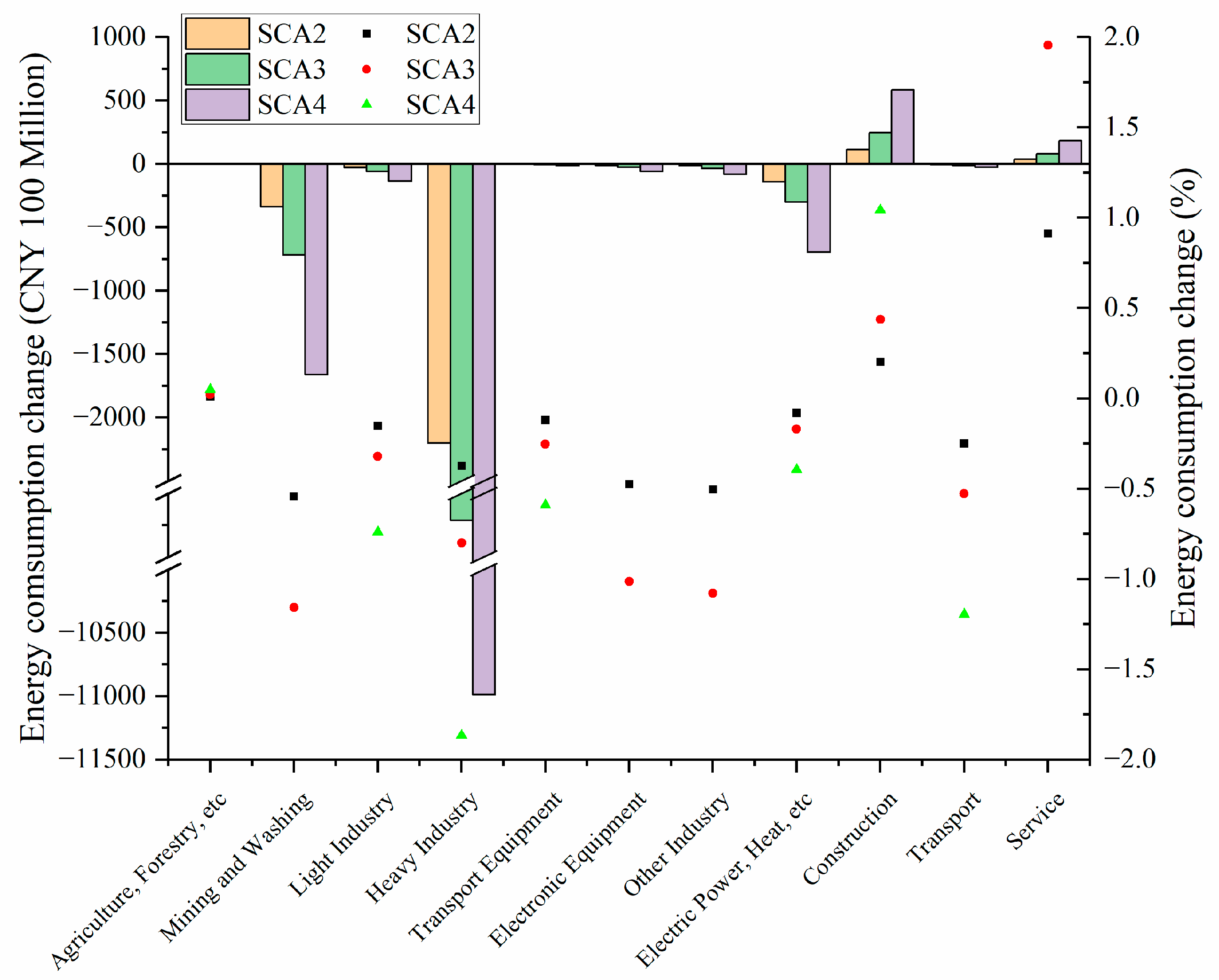
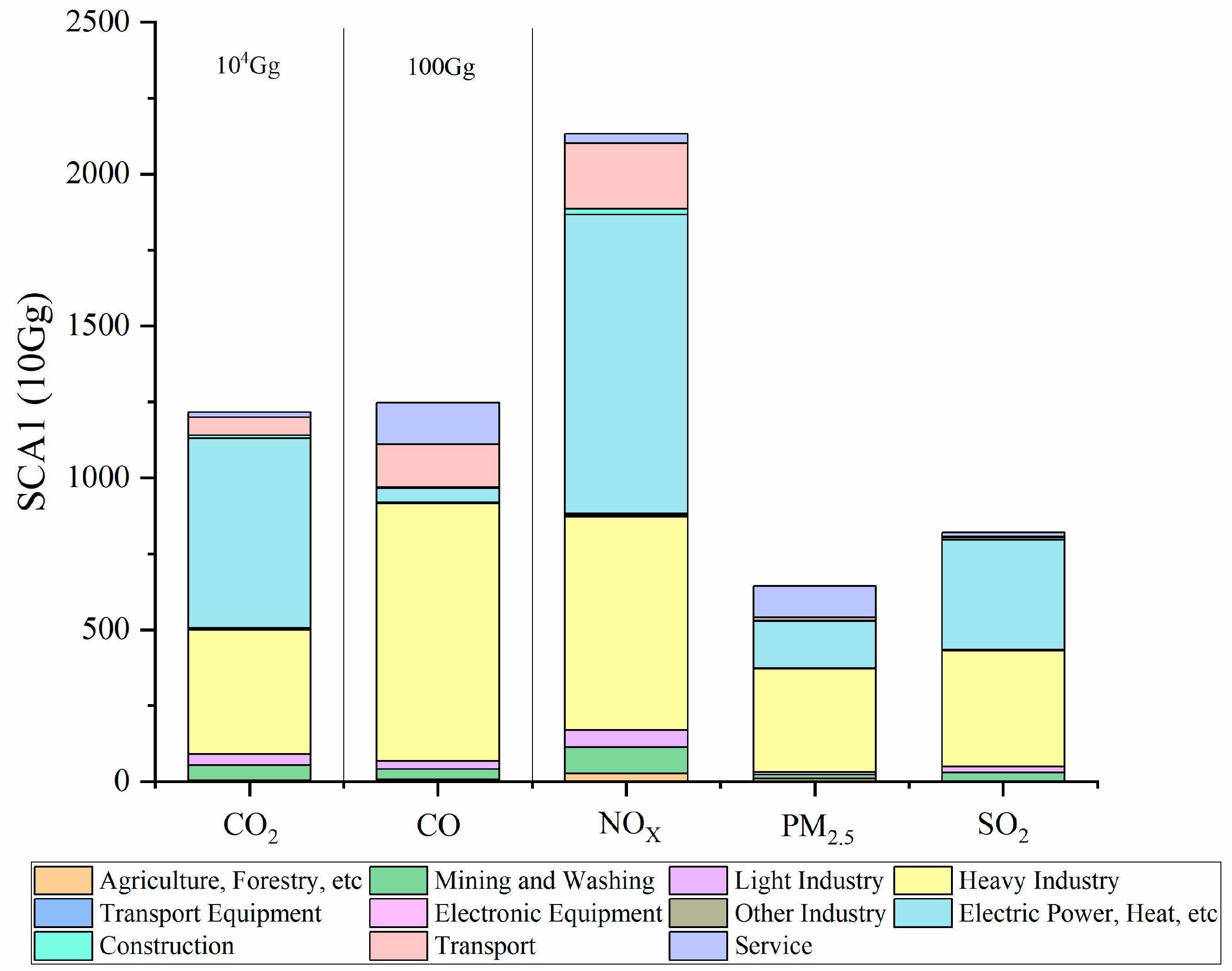
Figure 2 shows that compared with no resident tourism subsidy (SCA1), fixing the labor force and increasing resident tourism subsidies (SCA2, SCA3, and SCA4) have reduced energy consumption in most sectors, except the other service sectors and construction. Under all the resident tourism subsidy scenarios (SCA2, SCA3, and SCA4), the energy consumption of the heavy industry sector decreases the most, but the relative change is not the most significant, which is caused by the largest energy consumption being found in the heavy industry. In addition to industrial sectors, tourism subsidies have considerably reduced energy consumption in the mining and washing sector while minimally influencing the agriculture, forestry, etc. sector. In addition, under the benchmark scenario (SCA1), the sectoral emission contribution of each pollutant is shown in Figure 3.
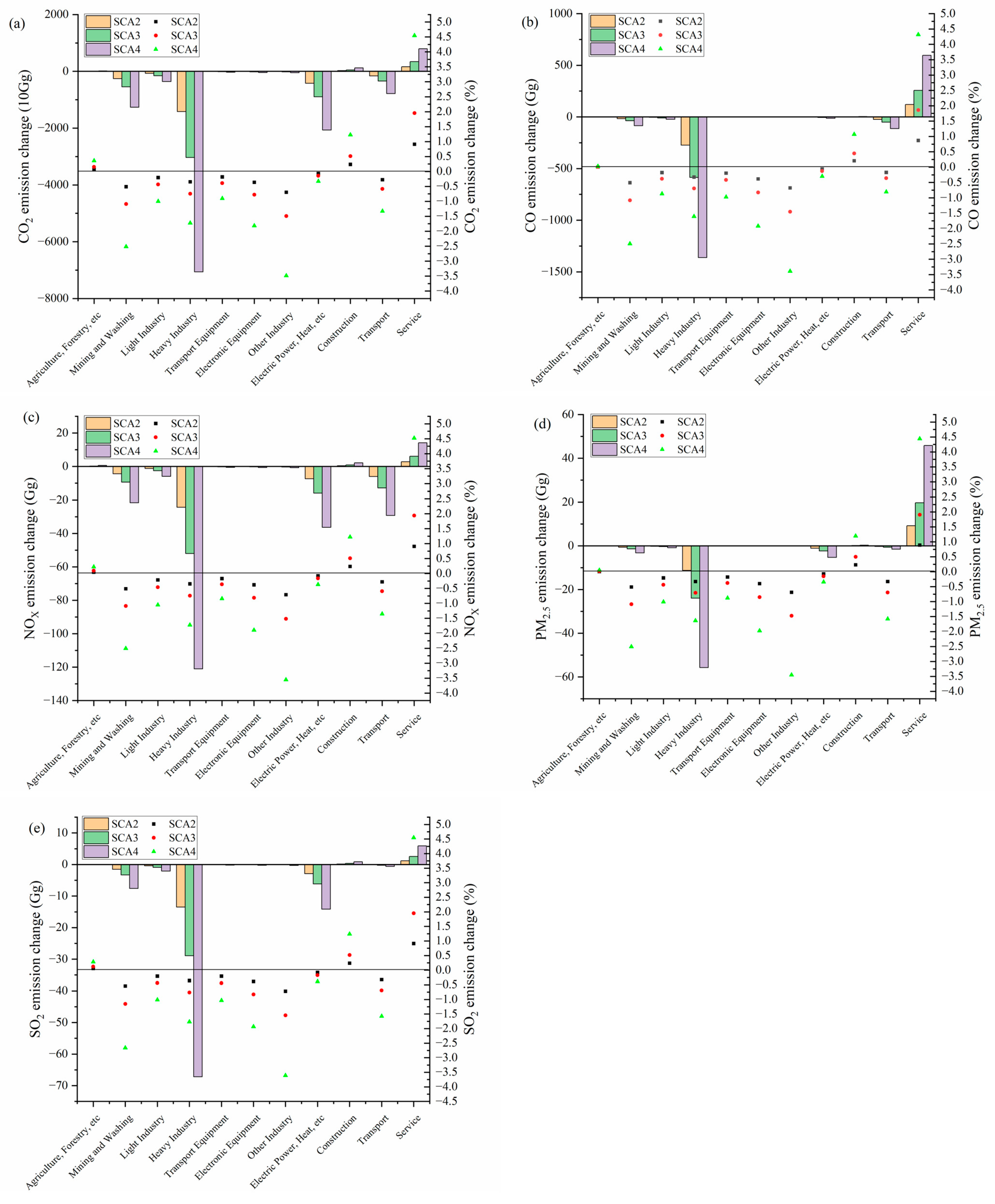
The sectoral emissions of CO2, CO, NOX, PM2.5, and SO2 are shown in Figure 4 under the assumption that there is no resident tourism subsidy (SCA1). It is clear that the heavy industry and electric power sectors are the main sources of CO2, NOX, and SO2 emissions; for CO emissions, the heavy industry sector is the largest emitter, accounting for more than 60% of total emissions; for PM2.5 emissions, the heavy industry, electric power, and service sectors are three major source sectors. The service industry also contributes significantly to CO and PM2.5 emissions, which both surpass 11%.
To analyze sectoral emission changes, this study compares SCA2, SCA3, and SCA4 scenarios (increased resident tourism subsidies of 5%, 10%, and 20%, respectively) with SCA1 (no resident tourism subsidy) in terms of CO2, CO, NOX, PM2.5, and SO2 (see Figure 4). The increases in sectors emissions for five atmospheric pollutants are typically commensurate with the changes in sectoral energy consumption (see Figure 2 and Figure 4). The sectors with larger energy consumption have greater emissions, while those with less energy consumption have less emissions. The energy consumption of the service sector increases by 0.91% under a resident tourism subsidy of 5% (SCA2), and the corresponding emissions of five typical atmospheric pollutants also increase respectively by 0.91%, 0.87%, 0.91%, 0.89%, and 0.91% (see details in Tables S9–S13). In the context of an increased resident tourism subsidy of 10% (SCA3), the service sector’s energy consumption is expanding at a 2.00% rate, and the emissions of CO2, CO, NOX, PM2.5, and SO2 increase by 1.95%, 1.86%, 1.94%, 1.91%, and 1.95%, respectively (see details in Tables S9–S13). In the more extreme scenario with a 20% resident tourism subsidy (SCA4), the energy consumption and emissions of each sector have close to proportional changes, and the growth rate in the service sector is 4.56%; the emissions of five typical atmospheric pollutants increase respectively by 4.54%, 4.32%, 4.52%, 4.44%, and 4.55% (see details in Tables S9–S13).
In general, with increasing resident tourism subsidy, the energy consumption and pollutant emissions of various sectors are decreasing. The heavy industry sector contributes the largest emission reduction of five typical atmospheric pollutants under SCA2, SCA3, and SCA4, which results from the greatest energy consumption reduction being in the heavy industry sector. We can see that although the energy consumption and CO2 emissions of the service sector, which are closely related to tourism, have increased, the energy consumption and CO2 emissions of energy-intensive industries such as heavy industries, mining and washing industries, and electric power, heat, etc. industries have decreased more significantly under resident tourism subsidies, finally resulting in a reduction in overall national emissions (see Table 3). In addition, as the service sector is closely related to PM2.5 emissions, the PM2.5 emissions of the service sector have increased significantly under the policy scenarios, which has caused there to be a relatively lower national emission reduction in PM2.5 (see Table 3).

4.3. Provincial Emission Changes

When there is no resident tourism subsidy (SCA1), the geographical distributions of CO2, CO, NOX, PM2.5, and SO2 emissions at the province level follow similar patterns. According to each province’s total energy consumption, Shandong and Hebei have the highest emissions, followed by Jiangsu, Guangdong, Henan, Anhui, and Guizhou (see Figure 5). Generally, provinces with larger economies of scale have more typical atmospheric pollutants emissions. However, Beijing and Shanghai have relatively low emissions due to the large proportion of the service sector in their economic structure.
The spatial changes in CO2, CO, NOX, PM2.5, and SO2 emissions among different resident tourism subsidy scenarios (SCA2, SCA3, and SCA4) are generally consistent with the national changes (see details in Figure 5). The regional changes in CO2 and NOX for varying air pollutants are similar across scenarios, with Shandong, Henan, and Inner Mongolia experiencing the biggest decreases. The CO2 emission reductions under the 5% resident tourism subsidy (SCA2) of these provinces can reach 6.53 Tg, 1.60 Tg, and 1.48 Tg, respectively, and the NOX emission reductions are 12.6 Gg, 3.05 Gg, and 2.22 Gg. Compared to CO2 and NOX, substantial reductions in CO emissions under SCA2 also occurred in Guizhou, Hunan, Hebei, and Anhui, which all exceeded 10 Gg. For SO2 emissions, 5% resident tourism subsidies have obvious impacts on Shandong (4.65 Gg) and Guizhou (1.74 Gg), followed by Shanxi (1.5 Gg) and Inner Mongolia (1.10 Gg), while reductions in PM2.5 are also significant in Hubei, Hunan, Yunnan, and Jiangsu. In the resident tourism subsidy scenarios, the large reduction of air pollutant emissions in Shandong, Hebei, and Guangdong is due to the significant decrease in energy usage in these provinces. In addition, some provinces, such as Shanxi and Inner Mongolia, have a large overcapacity of coal. The development of the tourism-related service sector may improve the economic structure of these provinces, reduce the output of coal-related industries, and lead to more emission reduction.
As a whole, the provinces with more energy consumption have greater emission reduction potential under such a policy, and higher resident tourism subsidies tend to cause more significant emission reductions. However, the increase or decrease in provincial emissions may not be generalized roughly; it needs to be further analyzed in combination with the actual energy consumption data and emission data of each province and each sector.

5. Discussion

In this study, a multiregional and multisector CGE model is developed to compare the effects of resident tourist subsidies on the economy and the environment in China in 2021. The benchmark scenario (SCA1: fixed total labor force and no resident tourism subsidy) and three subsidy policy scenarios (SCA2: fixed total labor force and with a resident tourism subsidy of 5%, SCA3: fixed total labor force and with a resident tourism subsidy of 10%, and SCA4: fixed total labor force and with a resident tourism subsidy of 20%) are set up.
The findings show that at the national level, with the total labor force stable, GDP, total investment, and total welfare are increasing with the increase in resident tourism subsidies (SCA2, SCA3, and SCA4). Previously, a study on tourism subsidy policies in Singapore [33] also came to the conclusion that tourism subsidies have a positive effect on the economy. Moreover, the emissions of CO2, CO, NOX, PM2.5, and SO2 decrease more significantly under the increase in resident tourism subsidies (SCA2, SCA3, and SCA4).
At the sector level, when the total labor force is fixed and the resident tourism subsidy is increased, the output of most sectors, except for the service sector, decreases compared with the benchmark scenario (SCA1). The changes in the emissions of CO2, CO, NOX, PM2.5, and SO2 in various sectors are basically consistent with the changes in output. Additionally, the heavy industry sector has the most significant decrease in energy consumption, which leads to the highest decrease in emissions of the five common atmospheric pollutants. The simulation results show that the labor force of many primary and secondary industries, especially the heavy industry sector and the mining and washing sector, migrates to the service sector under tourism subsidy, which means that the travel subsidy policy may have the potential to promote employment transfer. In the low-carbon transition of the energy structure, a large number of employment groups in traditional fossil energy and upstream and downstream industries face a crisis of income reduction, job transfer, and even unemployment [41]. Resident tourism subsidy policy can provide opportunities for these groups, protect the adversely affected labor force, and ensure that their basic rights and livelihoods are not negatively affected by low-carbon transition. This finding indicates that resident tourism subsidy can contribute to the Chinese just transition process. Li et al. [29] put forward a similar result in their study on the impact of tourism development on supply-side reform.
Regionally, under the baseline (SCA1), Shandong and Hebei have the highest regional CO2, CO, NOX, PM2.5, and SO2 emissions, followed by Guangdong, Jiangsu, Henan, Anhui, and Guizhou (due to their high levels of energy consumption). When the resident tourism subsidy is increased, the emission reduction of Shandong, Hubei, Hunan, and Guangdong is greater, which is due to the great reduction in energy consumption in these provinces. Moreover, the provinces with coal overcapacity, such as Shanxi and Inner Mongolia, achieve substantial emission reductions due to the changes in their economic structure.
We conduct five additional groups of scenario analyses to avoid the limitations of drawing conclusions only from SCA2, SCA3, and SCA4. The details of the scenario settings are supplied in the Supplementary Materials (see details in Table S5). The changes in national GDP and national typical atmospheric pollutant emissions under the five comparison scenarios are shown in Figure 5. It can be seen that in all the comparison scenarios, the economic promotion effect increases with the increase in resident subsidies. Moreover, the emission reductions of national CO2, CO, NOX, PM2.5, and SO2 gradually increase under incrementally increased tourism subsidies.
The CGE model still has several restrictions and uncertainties, most of which have been covered in earlier research. Firstly, the sectoral and regional emissions are not entirely correct, which may alter how much the environment is impacted by resident tourism subsidies. Secondly, for dynamic modeling from 2007 to 2019, this study applies national resident tourism consumption data to replace the resident tourism consumption data of each province because the basic tourism consumption data of each province are incomplete. Furthermore, as tourism is a complex industry related to various sectors rather than a separate industry, the industry division and approach to policy implementation may affect the accuracy of the policy simulation results. As further data and measurements become available in the future, these problems will be addressed one at a time.

6. Conclusions

In summary, the CGE model in this article can simulate the scenarios of resident tourism subsidies and provide decisionmakers greater understanding of the effects of emissions and the economy on the province. The findings reveal that an increase in resident tourism subsidies promotes output growth in tertiary industries and significantly decreases the outputs of a number of secondary industries through crowding-out effects, while the overall growth of the national economy is improved. In addition, resident tourism subsidy can promote the inflow of labor from some high-energy-consumption sectors to the service sector, which is conducive to the just transition process. In terms of emission reduction, under resident tourism subsidy, the emissions of CO2, CO, NOX, PM2.5, and SO2 can be greatly reduced. Some provinces, such as Shandong, Guizhou, and Inner Mongolia, have shown great potential for emission reduction under such a policy. Based on these findings, it is credible that resident tourism subsidy policy will facilitate the construction of low-carbon development ideas and will be conducive to slowing global warming and helping achieve the Chinese carbon neutrality strategy. In facing the challenges of carbon neutrality and global temperature change in the new era, the Chinese government should consider more tourism subsidies in the transition to a green society to accelerate economic development while reducing air pollutant emissions.

Supplementary Materials

The following supporting information can be downloaded at: https://www.mdpi.com/article/10.3390/su15108351/s1, Figure S1: Simulations of national GDP and its growth rate from 2007 to 2030. Figure S2: Comparisons of simulation results (solid lines) of regional GDP with national statistics (dotted lines). Figure S3: Comparison between simulated (solid lines) industrial structure and national statistics (dotted lines). Figure S4: Comparison of simulated national NOX, SO2, CO2 and PM2.5 emissions with other emission inventory sources, including the National Statistics as well as the widely used emission inventory MEIC (http://www.meicmodel.org/). Figure S5: The regional absolute changes in energy consumption (million yuan) under SCA2, SCA3 and SCA3 compared to baseline (the SCA1 scenario). Figure S6: The regional absolute changes in output of heavy industry sector (million yuan) under SCA2 and SCA3 compared to baseline (the SCA1 scenario). Figure S7: The segmentation of tourism module in CGE model. Table S1: Definition of regions in the model. Table S2: Definition of sectors in the model. Table S3: Elasticities of production functions. Table S4: Elasticities in the commodities market. Table S5: Five additional sets of scenarios with fixed total labor force. Table S6: Sectoral output (values in the parentheses represent the percentage changes from SCA1) in 2021 under four scenarios (RMB, billion). Table S7: Sectoral labor input (values in the parentheses represent the percentage changes from SCA1) in 2021 under four scenarios (RMB, 100 million). Table S8: Sectoral capital input (values in the parentheses represent the percentage changes from SCA1) in 2021 under four scenarios (RMB, 100 million). Table S9: Sectoral CO2 emission (Gg) under SCA1, and the sectoral changes (Gg) in CO2 emission under SCA2, SCA3 and SCA4 compared to SCA1 (values in the parentheses represent the percentage of sectoral CO2 emission change from the total change). Table S10: Sectoral CO emission (Gg) under SCA1, and the sectoral absolute changes (Gg) in CO emission under SCA2, SCA3 and SCA4 compared to SCA1 (values in the parentheses represent the percentage of sectoral CO emission change from the total change). Table S11: Sectoral NOX emission (Gg) under SCA1, and the sectoral absolute changes (Gg) in NOX emission under SCA2, SCA3 and SCA4 compared to SCA1 (values in the parentheses represent the percentage of sectoral NOX emission change from the total change). Table S12: Sectoral PM2.5 emission (Gg) under SCA1, and the sectoral absolute changes (Gg) in PM2.5 emission under SCA2, SCA3 and SCA4 compared to SCA1 (values in the parentheses represent the percentage of sectoral PM2.5 emission change from the total change). Table S13: Sectoral SO2 emission (Gg) under SCA1, and the sectoral absolute changes (Gg) in SO2 emission under SCA2, SCA3 and SCA4 compared to SCA1 (values in the parentheses represent the percentage of sectoral SO2 emission change from the total change). Table S14: Regional CO2 emission (Gg) (values in the parentheses represent the percentage changes from SCA1) in 2020 under SCA1, SCA2, SCA3 and SCA4 scenarios. Table S15: Regional CO emission (Gg) (values in the parentheses represent the percentage changes from SCA1) in 2020 under SCA1, SCA2, SCA3 and SCA4 scenarios. Table S16: Regional NOX emission (Gg) (values in the parentheses represent the percentage changes from SCA1) in 2020 under SCA1, SCA2, SCA3 and SCA4 scenarios. Table S17: Regional PM2.5 emission (Gg) (values in the parentheses represent the percentage changes from SCA1) in 2020 under SCA1, SCA2, SCA3 and SCA4 scenarios. Table S18: Regional SO2 emission (Gg) (values in the parentheses represent the percentage changes from SCA1) in 2020 under SCA1, SCA2, SCA3 and SCA4 scenarios. Table S19: The regional absolute changes in energy consumption (10 million yuan) under SCA2, SCA3 and SCA4 compared to baseline (the SCA1 scenario), and the energy consumption per region (billion yuan) under SCA1. Table S20: The regional absolute changes in output of heavy industry sector (10 million yuan) under SCA2, SCA3 and SCA4 compared to baseline (the SCA1 scenario), and the output of heavy industry sector per region (billion yuan) under SCA1. References [31,38,39,40,42] are cited in the Supplementary Materials.

Author Contributions

Methodology, L.Z., Q.Y., Y.W. (Yuqing Wang) and Y.L.; software, X.H.; validation, Y.W. (Yuqing Wang); formal analysis, L.Z.; investigation, L.Z., Q.Y. and X.H.; resources, Q.Y., Y.W. (Yuqing Wang), X.H., X.W. (Xuejun Wang), J.M. and S.T.; writing—original draft preparation, L.Z.; writing—review and editing, J.L., Y.L, J.H., Y.W. (Yi Wan), X.W. (Xuejun Wang), J.M., X.W. (Xilong Wang) and S.T.; visualization, Y.L. and S.T.; supervision, J.L., J.H., Y.W. (Yi Wan), X.W. (Xuejun Wang), J.M., X.W. (Xilong Wang) and S.T.; funding acquisition, J.H., Y.W. (Yi Wan) and X.W. (Xilong Wang). All authors have read and agreed to the published version of the manuscript.

Funding

This work was supported by funding from the National Natural Science Foundation of China (under grand nos. 42077196 and 41821005).

Institutional Review Board Statement

Not applicable.

Informed Consent Statement

Not applicable.

Data Availability Statement

The authors confirm that the data supporting the findings of this study are available within the article and its Supplementary Materials.

Conflicts of Interest

The authors declare no conflict of interest.

References

  1. Newell, P.; Mulvaney, D. The political economy of the ‘just transition’. Geogr. J. 2013, 179, 132–140. [Google Scholar] [CrossRef]
  2. Evans, G.; Phelan, L. Transition to a post-carbon society: Linking environmental justice and just transition discourses. Energy Policy 2016, 99, 329–339. [Google Scholar] [CrossRef]
  3. Dalglish, C.; Leslie, A.; Brophy, K.; Macgregor, G. Justice, development and the land: The social context of Scotland’s energy transition. Landsc. Res. 2018, 43, 517–528. [Google Scholar] [CrossRef]
  4. Snell, D. ‘Just transition’? Conceptual challenges meet stark reality in a ‘transitioning’ coal region in Australia. Globalizations 2018, 15, 550–564. [Google Scholar] [CrossRef]
  5. Cock, J. Resistance to coal inequalities and the possibilities of a just transition in South Africa. Dev. South. Afr. 2019, 36, 860–873. [Google Scholar] [CrossRef]
  6. Harrahill, K.; Douglas, O. Framework development for ‘just transition’ in coal producing jurisdictions. Energy Policy 2019, 134, 110990. [Google Scholar] [CrossRef]
  7. Cha, J.M. A just transition for whom? Politics, contestation, and social identity in the disruption of coal in the Powder River Basin. Energy Res. Soc. Sci. 2020, 69, 101657. [Google Scholar] [CrossRef]
  8. Moodie, J.; Tapia, C.; Löfving, L.; Gassen, N.S.; Cedergren, E. Towards a Territorially Just Climate Transition—Assessing the Swedish EU Territorial Just Transition Plan Development Process. Sustainability 2021, 13, 7505. [Google Scholar] [CrossRef]
  9. Wu, P.; Shi, P. An estimation of energy consumption and CO2 emissions in tourism sector of China. J. Geogr. Sci. 2011, 21, 733–745. [Google Scholar] [CrossRef]
  10. Wang, K.; Li, J.; Xi, J. Linking between Carbon Dioxide Emission and Tourism Economic Growth in China. Tour. Trib. 2014, 29, 24–33. [Google Scholar]
  11. Yu, X.; Tian, G.; Sun, X.; Lai, C. Contribution of Tourism to National Economy Based on Input-output Model. World Sci.-Tech. R D 2014, 36, 432–438. [Google Scholar]
  12. Shi, P.H. On the Evaluation of Regional Development of China’s Tourism Employment. Tour. Trib. 2003, 18, 45–51. [Google Scholar]
  13. Li, L.; Li, J.; Tang, L.; Wang, S. Balancing Tourism’s Economic Benefit and CO2 Emissions: An Insight from Input–Output and Tourism Satellite Account Analysis. Sustainability 2019, 11, 1052. [Google Scholar] [CrossRef]
  14. Williams, G. Economic Impacts from Development of the Coastal Town in Queensland on Tourism and Regional Economy. Resources 2016, 5, 48. [Google Scholar] [CrossRef]
  15. Kronenberg, K.; Fuchs, M.; Lexhagen, M. A multi-period perspective on tourism’s economic contribution—A regional input-output analysis for Sweden. Tour. Rev. 2018, 73, 94–110. [Google Scholar] [CrossRef]
  16. Cadarso, M.; Gómez, N.; López, L.A.; Tobarra, M.-Á. Calculating tourism’s carbon footprint: Measuring the impact of investments. J. Clean. Prod. 2016, 111, 529–537. [Google Scholar] [CrossRef]
  17. Camelia, S.; Razvan, S.M.; Zelia, B.; Ana-Irina, D. An Input-Output Approach of CO2 Emissions in Tourism Sector in Post-Communist Romania. In Proceedings of the International Conference Emerging Markets Queries in Finance and Business, Târgu Mureș, Romania, 24–27 October 2012. [Google Scholar]
  18. Zhou, D.; Yanagida, J.F.; Chakravorty, U.; Leung, P. Estimating economic impacts from tourism. Ann. Tour. Res. 1997, 24, 76–89. [Google Scholar] [CrossRef]
  19. Berrittella, M.; Bigano, A.; Roson, R.; Tol, R.S. A general equilibrium analysis of climate change impacts on tourism. Tour. Manag. 2006, 27, 913–924. [Google Scholar] [CrossRef]
  20. Dwyer, L. Computable General Equilibrium Modelling: An Important Tool for Tourism Policy Analysis. Tour. Hosp. Manag.-Croat. 2015, 21, 111–126. [Google Scholar] [CrossRef]
  21. Blake, A.; Durbarry, R.; Eugenio-Martin, J.L.; Gooroochurn, N.; Hay, B.; Lennon, J.; Sinclair, M.T.; Sugiyarto, G.; Yeoman, I. Integrating forecasting and CGE models: The case of tourism in Scotland. Tour. Manag. 2006, 27, 292–305. [Google Scholar] [CrossRef]
  22. Inchausti-Sintes, F. Tourism: Economic growth, employment and Dutch Disease. Ann. Tour. Res. 2015, 54, 172–189. [Google Scholar] [CrossRef]
  23. Ihalanayake, R. Economic effects of tourism tax changes in Australia: Empirical evidence from a computable general equilibrium model. Tour. Econ. 2012, 18, 181–202. [Google Scholar] [CrossRef]
  24. Meng, X.; Siriwardana, M.; Pham, T. A CGE assessment of Singapore’s tourism policies. Tour. Manag. 2013, 34, 25–36. [Google Scholar] [CrossRef]
  25. Ponjan, P.; Thirawat, N. Impacts of Thailand’s tourism tax cut: A CGE analysis. Ann. Tour. Res. 2016, 61, 45–62. [Google Scholar] [CrossRef]
  26. Gilliland, T.E.; Sanchirico, J.N.; Taylor, J.E. Market-driven bioeconomic general equilibrium impacts of tourism on resource-dependent local economies: A case from the western Philippines. J. Environ. Manag. 2020, 271, 110968. [Google Scholar] [CrossRef]
  27. Njoya, E.T.; Seetaram, N. Tourism Contribution to Poverty Alleviation in Kenya: A Dynamic Computable General Equilibrium Analysis. J. Travel Res. 2018, 57, 513–524. [Google Scholar] [CrossRef]
  28. Li, S.; Blake, A.; Cooper, C. Modelling the economic impact of international tourism on the Chinese economy: A CGE analysis of the Beijing 2008 Olympics. Tour. Econ. 2011, 17, 279–303. [Google Scholar] [CrossRef]
  29. Li, S.; Liu, A.; Song, H. Does tourism support supply-side structural reform in China? Tour. Manag. 2018, 71, 305–314. [Google Scholar] [CrossRef]
  30. Zhang, J.; Zhang, Y. Carbon tax, tourism CO2 emissions and economic welfare. Ann. Tour. Res. 2018, 69, 18–30. [Google Scholar] [CrossRef]
  31. Zhang, J.; Zhang, Y. Chinese tourism economic change under carbon tax scenarios. Curr. Issues Tour. 2020, 23, 836–851. [Google Scholar] [CrossRef]
  32. Schubert, S.F.; Brida, J.G. Dynamic effects of subsidizing the tourism sector. Tour. Econ. 2008, 14, 57–80. [Google Scholar] [CrossRef]
  33. Meng, X. Is a Tourism Subsidy the Best Response to the Global Financial Crisis? A Short-run CGE Simulation for Singapore. Asia Pac. J. Tour. Res. 2014, 19, 325–341. [Google Scholar] [CrossRef]
  34. Meng, S.; Pham, T.; Dwyer, L.; Grant, B. Carbon Price Impacts on the Chinese Tourism Industry. J. Travel Res. 2020, 60, 370–383. [Google Scholar] [CrossRef]
  35. Bergman, L. A System of Computable General Equilibrium Models for A Small Open-Economy. Math. Model. 1982, 3, 421–435. [Google Scholar] [CrossRef]
  36. Zhang, X. Principles of Computable General Equilibrium (CGE) Modeling and Programming; Gezhi Publishing House: Shanghai, China, 2010. [Google Scholar]
  37. Lfgren, H.; Harris, R.L.; Robinson, S. A Standard Computable General Equilibrium (CGE) Model in GAMS; TMD Discussion Papers; International Food Policy Research Institute (IFPRI): Washington, DC, USA, 2001. [Google Scholar]
  38. Hu, X.; Sun, Y.; Liu, J.; Meng, J.; Wang, X.; Yang, H.; Xu, J.; Yi, K.; Xiang, S.; Li, Y.; et al. The impact of environmental protection tax on sectoral and spatial distribution of air pollution emissions in China. Environ. Res. Lett. 2019, 14, 054013. [Google Scholar] [CrossRef]
  39. Yang, Q.; Hu, X.; Wang, Y.; Liu, Y.; Liu, J.; Ma, J.; Wang, X.; Wan, Y.; Hu, J.; Zhang, Z.; et al. Comparison of the impact of China’s railway investment and road investment on the economy and air pollution emissions. J. Clean. Prod. 2021, 293, 126100. [Google Scholar] [CrossRef]
  40. Liu, S. Ten Years Prospect of China’s Economic Growth: Forming a New Normal of Growth in the Process of Reform; China CITIC Press: Beijing, China, 2014. [Google Scholar]
  41. Zhang, Y.; Ji, X.-R.; Wang, M. Just transition in climate regime: Concept development and governance progress. Progress. Inquisitiones Mutat. Clim. 2021, 17, 245–254. [Google Scholar]
  42. Jin, C. The Impact of China's Transportation Infrastructure on the National Economy. Master’s Thesis, Beijing Jiaotong University, Beijing, China, 2019. [Google Scholar]
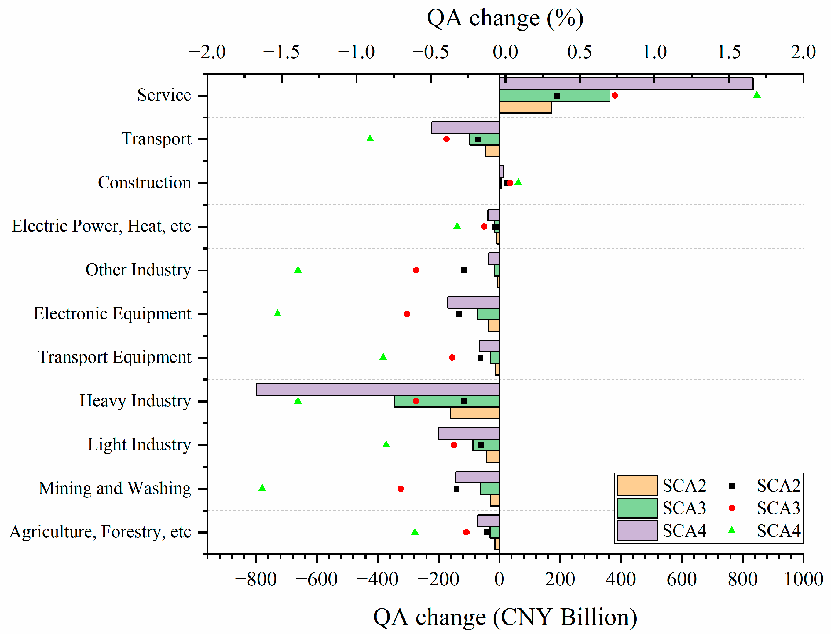
Figure 1. The absolute changes (colored bars, CNY 100 million) and relative changes (colored scatters, %) in sectoral output (QA) under SCA2 (resident tourism subsidy of 5%, orange bars and black squares), SCA3 (resident subsidy of 10%, green bars and red dots), and SCA4 (resident subsidy of 20%, purple bars and green triangles) compared to benchmark scenario SCA1 (no tourism subsidy).
Sustainability 15 08351 g001
Figure 2. The absolute changes (colored bars) and relative changes (colored scatters) in sectoral energy consumption under SCA2 (resident tourism subsidy of 5%, orange bars and black squares), SCA3 (resident subsidy of 10%, green bars and red dots), and SCA4 (resident subsidy of 20%, purple bars and green triangles) compared to the benchmark scenario SCA1 (no resident tourism subsidy).
Sustainability 15 08351 g002
Figure 3. Total sectoral emissions and their composition of emissions by sector of multiple air pollutants in 2021 under the benchmark scenario SCA1 (no resident tourism subsidy), including CO2 (104 Gg), CO (100 Gg), NOX (10 Gg), PM2.5 (10 Gg), and SO2 (10 Gg).
Sustainability 15 08351 g003
Figure 4. The sectoral absolute changes (colored bars) and relative changes (colored scatters) of (a) CO2, (b) CO, (c) NOX, (d) PM2.5, (e) SO2 emissions under SCA2 (resident tourism subsidy of 5%, orange bars and black squares), SCA3 (resident subsidy of 10%, green bars and red dots), and SCA4 (resident subsidy of 20%, purple bars and green triangles) compared to the benchmark scenario SCA1 (no resident tourism subsidy).
Sustainability 15 08351 g004
Figure 5. The provincial absolute emission impacts in CO2 (upper row), CO (second row), NOX (third row), PM2.5 (fourth row), and SO2 (bottom row) under benchmark scenario SCA1 in 2021 (no resident tourism subsidy) (first column), SCA2 (with a resident tourism subsidy of 5%) compared to benchmark scenario SCA1 (second column), SCA3 (with a resident tourism subsidy of 10%) compared to benchmark scenario SCA1 (third row), and SCA4 (with a resident tourism subsidy of 20%) compared to benchmark scenario SCA1 (fourth row). The second, third, and fourth columns of each row share the same legend.
Sustainability 15 08351 g005
Table 1. Under four scenarios, the national GDP, household welfare, and investment in 2021 (the amounts in parentheses show the percentage changes from SCA1, unit: CNY, 100 billion).
GDPEVInvestment
SCA1823299270
SCA2827 (0.41%)303 (1.6%)270 (0.032%)
SCA3831 (0.90%)306 (2.5%)270 (0.071%)
SCA4841 (2.1%)313 (4.8%)270 (0.181%)
Table 2. The sector impact on labor and capital change under different scenarios.
Industry (CNY Million)LaborCapital
SCA2SCA3SCA4SCA2SCA3SCA4
Agriculture, Forestry, etc.−24.3−52.0−120.74.69.721.7
Mining and Washing−27.7−59.1−137.0−141.7−303.7−710.1
Light Industry−17.2−36.5−83.1−77.4−166.7−395.0
Heavy Industry−55.4−117.9−271.2−336.8−724.5−1709.1
Transport Equipment−7.1−15.1−34.6−13.1−28.3−67.9
Electronic Equipment−16.0−34.1−78.3−112.1−240.6−564.7
Other Industry−4.5−9.5−21.9−42.6−91.8−217.3
Electric Power, Heat, etc.−3.7−8.0−18.2−10.5−23.2−58.1
Construction−4.2−8.6−18.244.895.6221.6
Transport−32.1−68.2−156.2−149.4−319.2−740.8
Other Service192.1408.9939.3836.81780.34084.6
Table 3. (a) Under four scenarios, national CO2, CO, NOX, PM2.5, and SO2 emissions in 2021 (values in parentheses represent the percentage changes from SCA1, unit: Tg). (b) Under three subsidy scenarios, national emission change per resident tourism consumption in 2021, unit: g/CNY.
(a)
CO2CONOXPM2.5SO2
SCA112164125216.438.20
SCA212,142 (−0.18%)125 (−0.16%)21 (−0.19%)6.43 (−0.07%)8.18 (−0.21%)
SCA312,117 (−0.38%)124 (−0.35%)21 (−0.40%)6.42 (−0.14%)8.16 (−0.45%)
SCA412,056 (−0.88%)124 (−0.81%)21 (−0.93%)6.41 (−0.32%)8.11 (−1.04%)
(b)
SCA2−95.01−0.891−0.176−0.0184−0.0755
SCA3−95.35−0.894−0.177−0.0185−0.0758
SCA4−96.21−0.902−0.179−0.0186−0.0767
Disclaimer/Publisher’s Note: The statements, opinions and data contained in all publications are solely those of the individual author(s) and contributor(s) and not of MDPI and/or the editor(s). MDPI and/or the editor(s) disclaim responsibility for any injury to people or property resulting from any ideas, methods, instructions or products referred to in the content.