Abstract
Urbanization and industrial development in the Juárez Valley, Chihuahua, Mexico, have led to the abandonment and loss of productive agricultural areas. However, the extent and dynamics of this phenomenon are not precisely known due to the lack of updated information. Therefore, it is necessary to geospatially represent these changes over time and predict their probability of persistence into the future to provide decision-making tools for this border region of Mexico. Landsat images were processed, and random forest was applied as a classifier to obtain land uses from 1980 to 2020. The Land Change Modeler options in Terrset™ were executed to generate land use changes, persistence and probabilities. Results showed that urban, built-up areas gained 19,962 ha by 2020 while crops lost 1675 ha. Agricultural permanence has been consolidated over time (persistence until 2020 of 0.83), but evidence suggests that this persistence will decrease in the future due to urbanization (decreasing to 0.59 by 2100). This could jeopardize the availability of primary products and food, lead to land abandonment and exacerbate socio-demographic expansion in this vulnerable region.
1. Introduction
Since the beginning of space exploration, humans have developed a wide range of remote sensing technologies that enable the capture and representation of information from the surface of the Earth. Currently, there is a constellation of platforms or artificial satellites orbiting the planet for various purposes, including SPOT, TERRA, Landsat missions, COPERNICUS, Galileo, MODIS and AQUA, among others [1,2]; these platforms are equipped with sensors that capture information from the Earth and store it in multispectral bands [3], enabling the monitoring of terrestrial space [4]. This facilitates the investigation and updating of historical cartographic documentation of natural and anthropic land cover, as noted by Ancira and Treviño [5], Aquino [6] and Persaud and Milián [7]; furthermore, González et al. [8] and Leija et al. [9] indicated that analyzing spatio-temporal dynamics can help determine the events that influence a change from one type of cover to another.
Esquivel et al. [10], Davila et al. [11] and Qu et al. [12] used GIS and satellite remote sensing to generate cartography of land use and the processes it has undergone over time. Pérez and Romo [13] analyzed the urban planning of Ciudad Juárez in its expansion process towards the southeastern region using GIS. They noted that the municipal government expanded the urban area towards the east, affecting the agricultural lands of the Juárez Valley. This is consistent with Mártinez et al.’s work [14] to determine the spatio-temporal dynamics of land use coverages using Landsat images. The municipal administration attempted to remedy this problem between 1986 and 1989 by limiting growth towards the Juárez Valley, but expansion continued towards the south.
Esquivel et al. [10] emphasized the importance of knowing the historical and current state of land cover and land use of social interest. They pointed out that the lack of comprehensive territorial planning favors urban expansion with deficiencies in infrastructure and services, particularly in remote or peripheral areas of the city that are constantly expanding, displacing agricultural areas. The irregular urban sprawl in the Juárez Valley is a problem identified by Esquivel et al. [10], Davila et al. [11], Pérez and Romo [13] and Mártinez et al. [14]. Agricultural extensions are threatened by encroaching land uses, which have caused cities to exponentially increase their growth rate since the industrial revolution, resulting in economic and territorial losses, abandonment of plots and invasion of agricultural land use over other coverages such as natural grasslands. These changes have created new ecosystemic problems [15].
The general aim of this study was to use GIS and satellite remote sensing (RS) technologies to address the problem of cartographic updates of land cover between 1980 and 2020 and the historical and current analysis of its losses, gains and permanence. Additionally, the study aimed to perform a prospective analysis towards 2100 of the state of urban and agricultural land cover over the Juárez Valley in Chihuahua, Mexico.
2. Data and Methods
2.1. Study Area
The study area (AOI, area of interest) is located in the Juárez Valley, which is situated in the municipality of Juárez (Figure 1) in the northern state of Chihuahua, Mexico. The area covers 962.08 km2, with coordinates ranging from −106.623° to −106.180° longitude and 31.784° to 31.228° latitude [16]. The altitude ranges from 1077 to 1817 m above sea level, with slopes ranging from 0° to 70° in small mountain ranges [17]. The Juárez Valley is located on the Juárez aquifer (key no. 0833), with an area of 3386.44 km2 [16].
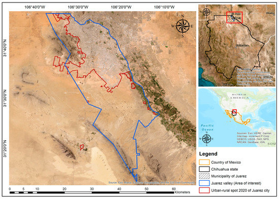
Figure 1.
Location of the area of interest (AOI) over the Juárez Valley in Chihuahua, Mexico. Source: own elaboration based on open data information [18].
The main land uses and vegetation in the area are urban, agricultural, pasture, and shrub secondary vegetation. There is rainfed and irrigated agriculture [18]. Cervantes and Montano [19], in their book El Valle de Juárez, mentioned that the main crops are alfalfa, sudan grass, pistachio, corn, wheat, cotton and sorghum, with regional environmental characteristics of average temperatures of 18.2 °C, a minimum of 7.5 °C and a maximum of 28.4 °C and an average annual precipitation of 265.3 mm and a population of 1,391,180 inhabitants as of 2015.
The processes used in this study (Figure 2) utilized satellite images hosted in the Google Earth Engine™ (GEE) data catalog provided in cooperation with the United States Geological Survey (USGS). This cloud-based petabyte geomatics platform allows for the processing, analysis and visualization of imagery from various satellite platforms such as Landsat’s historical legacy platform of ETM+, TM and OLI/TIRS sensors [20].
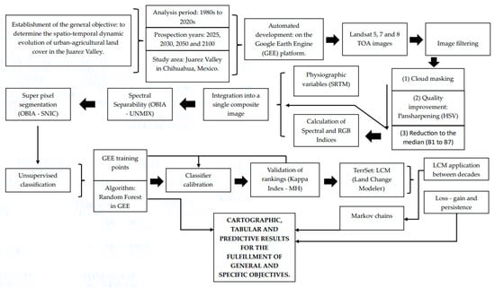
Figure 2.
Work flow diagram and the application of processes to obtain results and meet objectives. Source: own elaboration.
For the 1980s and 1990s, images were obtained for the Landsat 5 TM Collection Tier 1 mission calibrated for TOA (top of atmosphere) (LANDSAT/LT05/C02/T1_TOA courtesy of the U.S. Geological Survey) [21]. For the 2000s and 2010s, Landsat 7 Collection 2 Tier 1 mission imagery calibrated to TOA (top of atmosphere) (LANDSAT/LE07/C02/T1_TOA courtesy of the U.S. Geological Survey) was used [21]. The technical characteristics of these two platforms include a temporal resolution of 16 days, a multispectral band of 30 m, far infrared and thermal distances of 60 m and a Landsat 7 panchromatic band of 15 m, and their spectral ranges are from 0.45 to 2.35 μm [22]. For the 2020s, images from the Landsat 8 OLI/TIRS Collection 2 Tier 1 mission calibrated for TOA (top of atmosphere) (LANDSAT/LC08/C02/T1_TOA courtesy of the U.S. Geological Survey) were used [21]. The technical characteristics of this platform show a temporal resolution of 16 days operating under the same acquisition program as Landsat 5; the spatial resolution of the multispectral bands is 30 m, the panchromatic band of Landsat 8 is 15 m and its spectral ranges are from 0.443 to 1.375 nanometers [22,23].
Algorithms were developed on the GEE platform to analyze the multitemporal images. Date, boundary and cloud percentage filters were applied, and, subsequently, multispectral bands with spectral and spatial resolution were selected for the development of supervised and unsupervised classifications. Since the scenes available in the platform already have an atmospheric correction, this process was not applied. Date filters covering months with a lower percentage of cloud (<10%) were used next, and the boundaries (AOI) were loaded to the data warehouse and served as a mask file for extraction. Based on the filtered scenes, statistical reducers where the output is calculated per pixel were applied so that each pixel of the output was composed of the mean value of all images in the collection at that location (Figure 3) [20,21,22,23,24].

Figure 3.
Statistical reduction of the image collection to a single image. Source: Google Developers Data Catalog (2022) [20].
To obtain a multitemporal image, mosaics were generated. Images that did not comply with an acceptable percentage of cloudiness or coverage of the AOI of the studied regions were excluded, and cloud masking was applied using the quality band [25] to generate better-quality images. For platforms with a panchromatic band, the HSV pansharpening technique [26] was applied to increase the spatial resolution of the multispectral bands from 30 to 15 m.
For the Landsat 7 platform, the ETM+ sensor has an error from 2003 which causes banding or parallel lines and the absence of some information due to radiometric errors. To correct this drawback, interpolation and clustering techniques were applied following what was suggested by the USGS and EROS in 2004 [27].
A classification based only on spectral variables can show confusion among objects with similar spectral responses. Spectral indices [27,28] of vegetation, soil, water or even indices based on RGB (red, green and blue) [29] were used to discriminate pixels that could conflict in their spectral response. Among the indices used (Table 1) to discriminate the pixels that could conflict in their spectral response, NDVI, GNDVI, EVI, AVI, SAVI, NDMI, MSI, GCI, BSI, NDWI, NDSI, NDSI and VARI were calculated by map algebra using the corresponding bands. The wavelength covered by each band per satellite platform varies; for example, it is not the same wavelength for Landsat 5 band 1 (blue) as for Landsat 8 band 1 (coastal aerosol). For the RGB indices, NGRDI, GLI and VDVI were calculated according to what Poley and McDermin mentioned [30].

Table 1.
List of indexes calculated for multispectral and RGB images. Source: own elaboration based on USGS (2022) [27], Santos et al. (2022) [28], Roque (2021) [29] and the index database documented by IDB project (2011–2023) available at: https://www.indexdatabase.de/db/ia.php (accessed on 20 January 2023).
Physiographic variables were generated to support the classifier and indicate to the pixel its topographic or geographic position in the terrain [31]. This information helps the classifier to recategorize a pixel in relation to its neighboring pixels by the value of its topographic position if it has the same spectral response and value in an index. A DEM (digital elevation model) obtained from the NASA-USGS (USGS/SRTMGL1_003 courtesy of the U.S. Geological Survey) was used for this purpose. This is a SRTM (shuttle radar topography mission) [32] product with a spatial resolution of 30 m. The slopes and slope orientation variable were generated in degrees [33].
As the first training and calibration variables, spectral separability was performed at the pixel level from an unmixing with the end members of each class (Table 2). A transposed pseudo-inverse matrix was used to calculate the composite image for each class with the same number of bands. This technique is used in OBIA (object-based image analysis) [34,35].
Table 2.
Structure of a matrix for OBIA and spectral separability. Source: own elaboration.
To complement the OBIA processes, a segmentation of the physical and spectral characteristics representative of the objects that may contain the pixels was performed [36]. The composite image was segmented into polygons of objects corresponding to their spectral and index values, shape and texture. Neighborhood groupings were integrated in this process, which are based on spatial contiguity and correspondence. This analysis determines if the behavior of a pixel is similar to its neighbor in its vertical, horizontal and vertex limits [37,38]. The integral efficiency analysis allows for accurate discrimination for the identification of objects and generation of training polygons based on statistics and geospatial behavior.
To train the classification algorithm, training points were generated by photointerpretation and the values corresponding to the spectral signatures that best represented each class or object. The identified classes were Crops, Urban, Sands and Livestock. The machine learning prediction algorithm of random forest [39,40] available in GEE was used. It was executed with a number of decision trees [39] and the training points generated for each year and the variables or bands integrated in a single image.
The validation process consisted of comparing the results of the predictions or classifications against a set of independent data and calculating the kappa index that measures the level of agreement. This index allows us to know the degree to which the observers have certainty in their measurements or predictions [41]. The results of the kappa index (Equation (1)) are obtained by subtracting a proposed theoretical contribution given to randomness (Equation (3)) from reliability. This yields a result that is less than the overall reliability (Equation (2)). For categorical mapping, a significant percentage of the random map should be correct for user agreement [42].
where Po = proportion of the area correctly classified (overall reliability), and Pc = reliability resulting at random. Source: own elaboration based on Mas et al. [42].
Table 3 shows the basic structure of a confusion matrix of size n for the comparison of the georeferenced and map sites.
Table 3.
Basic structure to generate a confusion matrix for the calculation of the Kappa index. Source: own elaboration based on Mas et al. [42].
The results obtained for each period of each year were processed using a desktop GIS. The final layers were generated, and areas in hectares were calculated while isolating the land covers of interest. Formats for the classifications were prepared for their subsequent analysis in image processing software in the Land Use Change Modeler.
The LCM (Land Change Modeler) module was used to obtain the trends of land use change coverages, which allow for the mapping of transitions, permanences, losses and gains. The probability of change was calculated through Markov chains [43,44,45] for the years 2025, 2030, 2050 and 2100 using 1980 as the base year and 2020 as the final and starting consecutive years to be predicted.
To generate the models, the input parameters were the results of each year with a normalized legend by ID and category. The first LCM result was calculated by overlapping the pixels of each category of the initial year against that of the end year. The units shown were indicated in pixel units, hectares or others.
From these options, cartographic results of losses, gains, persistence and transitions were constructed for each analyzed period and the historical period [46,47]. Finally, with the information stored in each of the models, tables of Markov chains or probability of future change were obtained [48,49].
2.2. Statistical Analysis
The GEE platform was used to call collections by their identifier corresponding to the Landsat 5, 7 and 8 platforms and filtered by dates and area of interest. For 1980, it was a collection from 22 August 1982 to 1 May 1985, depending on image availability and cloud percentage (<10%). The multispectral bands to be used were selected, and this process was repeated for the other platforms, modifying the date filter. For 1990, it was from 1 January to 31 December 1990. For 2000, 2010 and 2020, a mosaic was generated, and a statistical reducer was applied to the median.
The quality of the filtered images was improved by optimizing the value of the pixels through a masking operation, selecting the quality statistics band and a bit-by-bit operation [50]. The HSV technique of pansharpening, used by Poveda et al. [26], was applied to the platforms that had a panchromatic band of 15 m spatial resolution. The necessary bands to construct the spectral indices were selected, as indicated by Santos et al. [28] and Roque [29]. The equations of the University of Bonn portal were accessed and solved by means of an expression in map algebra. The necessary bands to construct the spectral indices were selected [31], and slope variables in degrees and slope orientation [33] were constructed using the SRTM DEM.
For the OBIA spectral separability analysis, the spectral bands of the image, indexes and physiographic variables were integrated into a single, multiband image according to Ela and Claire [34] and Ramandhan et al. [35]. The SNIC (simple non-iterative clustering) algorithm was used for segmentation, and a reducer was applied to the clustering band [36,37,38].
In the final stage of the random forest (RF) classifier, the arguments from Phan et al. [39] and Amini et al. [40] were incorporated. An image composed of the bands obtained by unmixing, segmentation, physiographic and multispectral bands, their respective labels of each band with 500 decision trees [39] and the series of training points generated from a base sampling taken from Mas et al. [42] were used. This is a hybrid method combining systematic and clustering methods (MH). Ground truth points were obtained through photointerpretation and expert knowledge, representing each category of land use and vegetation analyzed.
The land use classifications for each year were validated using the kappa index and INEGI cartography scale 1:250,000, as indicated by Mas et al. [42]. Values were extracted from all series that were constant in their categories between 1980 and 2020. The sampling used the MH method, generating a 2000 × 2000 m grid with points created on each line at a distance of 15 m (133 points), to which points by clusters were added [42]. These were created within each polygon of the grid, where the minimum distance between them or the area of influence was 500 m so that each category or class within the quadrant had the same probability of being evaluated.
To run the LCM, classifications were spatially adjusted by resampling, ensuring that the spatial configuration was homogeneous in pixel size and number of columns and rows These were converted to ASCCI format for export to Terrset™ software and added to the soil change modeling processes in the LCM module, as mentioned by Anand and Ainam [43], Hamad et al. [44] and Sundara et al. [45]. Models were run for each decade between 1980 and 2020, and predictions of changes for the dates of 2025, 2030, 2050 and 2100 were obtained, feeding the processes of gains, losses and transitions [46,47] to obtain the net contributions through Markov chains [48,49].
3. Results
Figure 4 displays the land use and vegetation coverages represented before being generalized for the years 1980 and 2020. Urban land use is represented in black, built to the northwest of the AOI, and crops are shown in light green on the border strip of the Rio Bravo.
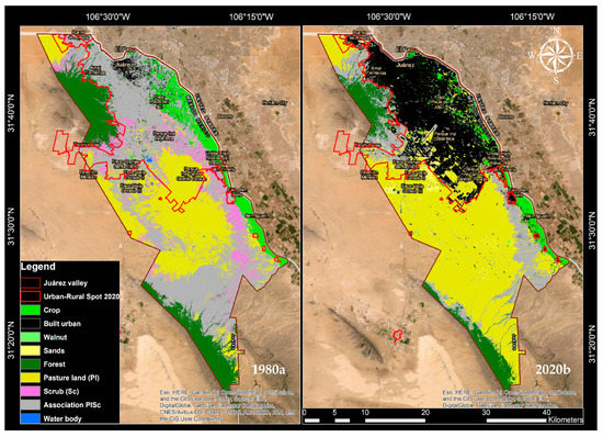
Figure 4.
Land use and vegetation classification in the Juárez Valley for the years 1980 (a) and 2020 (b). Source: own elaboration based on the results of the random forest classification.
The coverages were generalized into four classes: crops (crop, which integrates agricultural crops and walnut), built urban, sands (desert), and livestock (forest—forest, pasture land—pasture, scrub—scrub, association PlSc—association of pasture and scrub and water body—water bodies of small watering places). Table 4 shows the calculated areas in hectares for each of these classes for the years 1980 and 2020.
Table 4.
Hectares of generalized classes for the years 1980 and 2020. Source: own elaboration based on the results obtained from Figure 4.
Table 5 displays the changes and persistence in hectares for the historical period from 1980 to 2020.
Table 5.
Changes and persistence between classes for the period from 1980 to 2020 (C = changes, P = persistence). Source: own elaboration based on the results of the generalization of coverages to classes.
Figure 5 shows the classifications for the years 1990, 2000 and 2010 before they were grouped or generalized by classes.
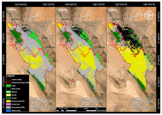
Figure 5.
Classification of land use and vegetation in the Juárez Valley for the years 1990 (a), 2000 (b) and 2010 (c). Source: own elaboration based on the results of the random forest classification.
Table 6 displays the areas in hectares for each of the classes for the years 1980 and 2020 based on the information in Figure 4.
Table 6.
Area in hectares of generalized classes for the years 1980 and 2020. Source: own elaboration.
Table 7 displays the cross-tabulation for these years, showing the area calculated in hectares for the change and persistence and the percentage of each of the categories in these years.
Table 7.
Cross-tabulation for the years 1990, 2000 and 2010. Source: own elaboration based on the results of the generalization of coverage to classes.
Figure 6 displays the years 1980, 1990, 2000, 2010 and 2020 with their four classes, where the green shades identify the cultivated areas, the black shades identify the built-up urban areas, the yellow shades identify the sandy areas and the brown shades identify the livestock areas.
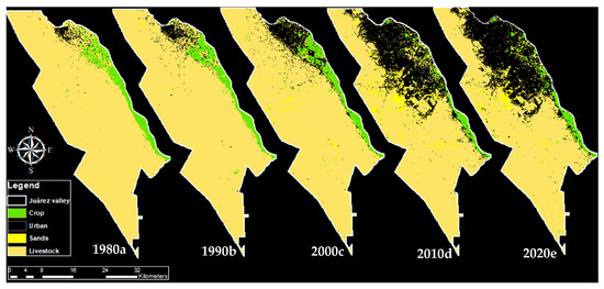
Figure 6.
Results of generalized cover for the years 1980 (a), 1990 (b), 2000 (c), 2010 (d) and 2020 (e). Source: own elaboration based on the results of the random forest classifications.
Figure 7 shows the multitemporal geospatial dynamics in hectares of change for the classes. It shows that the urban class experienced high growth demand over the other classes.
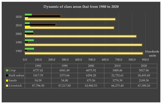
Figure 7.
Dynamics of the change in hectares for each class for each year analyzed. Source: own elaboration.
Table 8 displays the values of the validation matrix and kappa index for each validation year. For overall reliability, the lowest value was 0.72 for the year 2000, and the highest value was 0.92 for 1980. For random reliability, the lowest value was 0.70 for 2020 and the highest 0.99 for 2000.
Table 8.
Matrix with class values for points extracted from INEGI’s land use and vegetation series (GCP) and classifications with generalized classes for the years 1980, 1990, 2000, 2010 and 2020.
The values for kappa ranged from 0.44 for the year 2000 to 0.71 for 2020 (Table 9).
Table 9.
Values of the global and random reliability indicators and kappa index for each validation year. Source: own elaboration based on sampling and information from INEGI’s land use and vegetation series.
From the validated mapping of the classifications generated, grouping land cover or land use and vegetation into classes, it was possible to obtain the gains, losses and net contributions of the classes for the years 1980, 1990, 2000, 2010 and 2020. Table 10 and Table 11 shows the results in hectares for the historical period from 1980 to 2020.
Table 10.
Net losses, gains and contributions for each class from 1980 to 2020. Source: own elaboration.
Table 11.
Contributions in hectares between net profits and losses for each class in the period 1980–2020.
For the contributions in net hectares of gains or losses between classes for the period analyzed, a cartographic representation is shown for the net changes between classes (Figure 8, Figure 9 and Figure 10) in Table 6 and Table 7 for the period from 1980 to 2020.
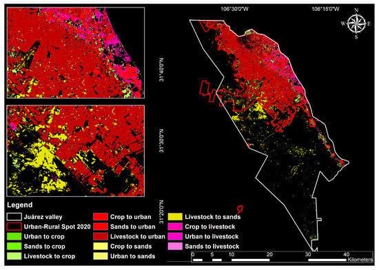
Figure 8.
Exchanges between classes for the historical period from 1980 to 2020. Source: own elaboration based on LCM results of the change analysis.
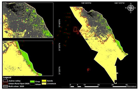
Figure 9.
Territorial persistence over time for the classes analyzed in the historical period from 1980 to 2020. Source: own elaboration based on LCM results and change analysis.
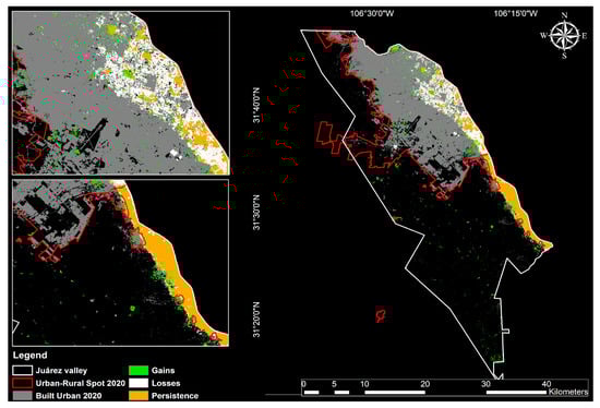
Figure 10.
Gains, losses and persistence of agricultural class or crops in the period from 1980 to 2020. Source: own elaboration based on LCM results and change analysis.
Figure 9 shows the class persistencies for the historical period from 1980 to 2020, and Figure 10 identifies the agricultural or crop gains, losses and persistencies for the same period.
Table 12 shows the net losses, gains and contributions in hectares.
Table 12.
Net losses, gains and contributions for each class between 1980 and 1990, 1990 and 2000, 2000 and 2010 and 2010 and 2020 (negative values in the third column indicate a gain): Source: prepared by the authors based on LCM processes.
Table 13 shows the contributions in hectares between net losses and gains for each class between 1980 and 1990, 1990 and 2000, 2000 and 2010 and 2010 and 2020.
Table 13.
Losses, gains and net changes for each class between the 1980s and 2020s.
Finally, Table 14 displays the prediction results of the Markov chains, which are change probability matrices generated from the historical period analyzed with the start year of 1980 and 2020 as the end year, and this result was taken as a starting point for the predictions for each of the years 2025, 2030, 2050 and 2100.
Table 14.
Markov chain matrix showing the probabilities of persistence (green) and changes (red) between classes based on the behavior of the historical period from 1980 to 2020 and from there to 2025, 2030, 2050 and 2100. Source: own elaboration with the results of the LCM analysis.
4. Discussion
In this study, geospatial techniques and tools in geographic information systems (GIS) and remote sensing (RS) were utilized to obtain historical land use information from the Juárez Valley. The results demonstrate that these technological trends allow for the obtaining of quality and certainty of results, which is consistent with previous studies by Su et al. [51] and Aguilar et al. [52] and Osuna et al. [53] and Figueredo and Rámon [54].
The increase in the consolidated or built urban area can be clearly observed in Figure 3 (historical period 1980 to 2020) and the intervals by decade (Figure 4 and Figure 5), which coincides with the analysis of Esquivel et al. [10], who analyzed this growth in terms of the impact on land use cover and its effects on the urban aquifer. This study determined that the areas most affected by urban sprawl growth were those corresponding to livestock land use (grassland–scrubland associations) that were found on the periphery of the urban sprawl for each decade, which is consistent with Fuentes [55] and the results of Graph 1 and Figure 4.
It was also detected that the agricultural and crop areas that developed towards the eastern region in the initial decade from 1980 to 2020 were consolidated as built urban areas, which was confirmed by Quijada and Chávez [56], indicating that this phenomenon has been registered since 1940, expanding the urban over flat areas, such as the agricultural areas located to the west of the city and which is reiterated in Pérez and Romo [13], an effect that is noted in the results of Figure 3, Figure 4 and Figure 5.
For the year 1980, between 6561.49 and 6737.42 ha of crop area were counted, while, for the year 2020, 5018.06 and 5027.06 ha were detected, with a loss of 1710.36 ha. This last result coincides with the problems mentioned by Martínez et al. [14] and was located and delimited by the municipal administration in 1986–1989. The previous result coincides with what was obtained and is framed cartographically in Figure 6 with the legend in red tones, where the change of crops towards the built urban in the historical period is shown. The net loss of crops is identified in Table 9, showing that it was a value of 1675 ha, while the net gain over all urban land uses was 19,962 ha between 1980 and 2020, where crops had a net contribution to the urban built-up area of 1773 ha in the historical period; this type of dynamic was also mentioned by Martínez et al. [14] in a region close to the Juárez Valley, that is, over the Rio Conchos basin.
Based on Table 13, the results of Figure 7 and Figure 8 (losses, gains and persistence and their respective tables) are supported, where the agricultural land use indicated 0.83 persistence towards 2025, with probabilities less than 0.01 of change to other classes. By 2030, these increased to 0.11 for the urban and livestock classes, while its permanence decreased to 0.78. This decrease was reflected in the year 2050, where its persistence resided at 0.60, and, for the changes, it indicated a probability of 0.22 for the urban class and 0.18 for livestock. For 2100, these continued to increase, from agricultural to urban with a change of 0.42 and 0.21 from agricultural to livestock, with the persistence of agricultural having a value of 0.28. These results coincide with those mentioned by Ramos et al. [57], who, although they did not work on the same area, obtained similar results of probability of land use change to urban by 2030.
The results of this study coincide with the hypothesis of the work of Pérez and Romo [13], where they indicated the relevance of urban growth in the borders since the 1960s, adding infrastructure planning problems, specifically in the southeastern area of Ciudad Juárez, where it is also indicated that this expansion/urbanization and effect are applied to agricultural or crop land uses.
To explain the permanence and consolidation of agricultural and cultivation plots in the study area, reference can be made to the findings of Ascencio et al. [58], which indicated that some relevant factors for this phenomenon may be the means of production, the characteristics of these and the valuation and development of the land, as well as the integration of productive systems. Therefore, this type of study opens a panorama to continue analyzing the study area and identify the processes that allow permanence to be offered to this type of productive system, which is of great importance for the population.
5. Conclusions
The objectives of this study were successfully achieved by employing geographic information systems and the use of satellite products, which proved to be a powerful support tool for monitoring land use changes in border regions such as the Juárez Valley, where the socio-economic phenomena associated with urbanization in recent years are significant and unfortunately have captured the world’s attention. The first objective was to generate the historical cartography—updated by decade (1980–2020)—of the main land uses and coverages for the region of the Juárez Valley in Chihuahua, Mexico, which was accomplished. From this, the second objective was fulfilled by calculating the areas of gains, losses and transitions and their respective mapping. It was found that the greatest growth occurred in the decade from 1990 to 2000 and in 2010, evidencing continuous urban growth since 1980 in areas of livestock use (associations of pasture–scrubland) to the south and west in agricultural regions.
The study showed that agricultural land use was consolidated, with plots that were not initially productive being grouped within the same zone and cultivated. Additionally, the border between agriculture and livestock increased towards the south, with the latter being adapted as a region of agricultural production. The third objective relating to the probabilities of persistence of the agricultural productive region in the future was fulfilled and indicated that, in the years analyzed, this will decrease. Urbanization is the main land use that can influence this type of loss, which represents a possible productive decrease, thus affecting the availability of primary products and food and income of the producers and can lead to land abandonment and problems for socio-demographic expansion.
Given what was generated and obtained in this study, it is advisable to continue analyzing the dynamics of land use changes, characterizing the activities that are being developed in the region and encouraging the collection of field information for better classification and validation of the information analyzed. Therefore, greater financing of this type of study is demanded by institutions involved in the planning and managing of territorial development so that they can benefit from more and better tools for decision making and solving problems associated with the phenomenon of urbanization, loss of productive activities and the degradation of natural resources in these border areas of developing countries such as Mexico.
Author Contributions
Conceptualization, M.E.E.-V. and M.d.R.B.-G.; Software, M.I.U.-C.; Validation, M.E.E.-V. and M.d.R.B.-G.; Formal analysis, M.I.U.-C. and E.S.-E.; Investigation, C.M.-D. and E.S.-E.; Writing—original draft, O.G.-C.; Writing—review & editing, M.I.U.-C. and E.S.-E.; Supervision, C.M.-D. and E.S.-E.; Project administration, C.M.-D. and O.G.-C. All authors have read and agreed to the published version of the manuscript.
Funding
This research received no external funding.
Data Availability Statement
Not applicable.
Conflicts of Interest
The authors declare no conflict of interest.
References
- The European Space Agency. Available online: https://www.esa.int/Space_in_Member_States/Spain/Constelacion_de_satelites (accessed on 20 January 2023).
- Moya, Z.J. Procesamiento GNSS en el marco geodésico CR-SIRGAS: Influencia de las épocas de observación y referencia. Rev. Univ. Costa Rica 2022, 32, 48–85. [Google Scholar]
- Universidad de Murcia. Available online: https://www.um.es/geograf/sig/teledet/fundamento.html (accessed on 20 January 2023).
- Veneros, J.; García, L.; Morales, E.; Gómez, V.; Torres, M.; López, M.F. Application of remote sensors for the analysis of vegetation cover and water bodies. IDESIA 2020, 38, 99–107. [Google Scholar] [CrossRef]
- Ancira, S.L.; Treviño, G.E. Using satellite images for forest management in northeast Mexico. Madera Y Bosques 2015, 21, 77–91. [Google Scholar]
- Aquino, I.V. Análisis Espacio-Temporal del Cambio de uso de Suelo por Expansión Urbana-Migración Deforestación en el Suelo de Conservación del Distrito Federal. Master’s Thesis, CentroGeo, Mexico City, Mexico, 6 June 2016. [Google Scholar]
- Persaud, H.; Milián, I. Eficiencia de las imágenes de radar para el monitoreo a tiempo casi real de bosques tropicales en Guyana. Arnaldoa 2021, 28, 577–592. [Google Scholar]
- González, G.S.; Nájera, G.O.; Murray, N.R.; Marceleño, F.S. Dinámica espacio-temporal de la cobertura y uso del suelo en una cuenca hídrica. CIBA 2016, 5, 29–42. [Google Scholar]
- Leija, E.G.; Pavón, N.P.; Sánchez, G.R.; Ángeles, P.G. Dinámica espacio-temporal de uso, cambio de uso y cobertura de suelo en la región centro de la Sierra Madre Oriental: Implicaciones para una estrategia REDD+ (Reducción de Emisiones por la Deforestación y Degradación). Rev. Cart. 2020, 102, 43–68. [Google Scholar] [CrossRef]
- Esquivel, C.V.; Alatorre, C.L.; Robles, M.A.; Bravo, P.L. Urban growth of Ciudad Juárez Chihuahua (1920–2015): Hypothesis about impacts on the land use and land cover and depletion of the urban aquifer. Acta Univ. 2019, 29, 1–29. [Google Scholar]
- Dávila, R.A.; Alatorre, C.L.; Bravo, P.L. Spatio-temporal evolution analysis of urban land use in the metropolis of Chihuahua. Econ. Soc. Y Territ. 2021, 21, 1–27. [Google Scholar]
- Qu, L.; Chen, Z.; Li, M.; Wang, H. Accuracy Improvements to Pixel-Based and Object-Based LULC Classification with Auxiliary Datasets from Google Earth Engine. Remote Sens. 2021, 13, 453. [Google Scholar] [CrossRef]
- Pérez, P.L.; Romo, A.M. Urban development plans: Instruments of legitimation in the urban expansion of Ciudad Juarez, Chihuahua. Estud. Demográficos Y Urbanos 2022, 37, 85–120. [Google Scholar] [CrossRef]
- Martínez, S.A.; Villanueva, D.J.; Estrada, A.J.; Vázques, V.C.; Orona, C.I. Soil loss and runoff modification caused by land use change in the Conchos river basin, Chihuahua. Nova Sci. 2021, 12, 25. [Google Scholar]
- Agenccias Europea de Medio Ambiente. Available online: https://www.eea.europa.eu/es/senales/senales-2015/articulos/la-agricultura-y-el-cambio-climatico (accessed on 20 January 2023).
- Secretaría de Medio Ambiente y Recursos Naturales. Available online: https://sigagis.conagua.gob.mx/ (accessed on 16 November 2022).
- Continuo de Elevaciones Mexicano. Available online: https://www.inegi.org.mx/app/geo2/elevacionesmex/ (accessed on 16 November 2022).
- Portal de Geoinformación. Continuo de Elevaciones Mexicano. 2022. Available online: http://www.conabio.gob.mx/informacion/gis/ (accessed on 9 November 2022).
- Cervantes, R.E.; Montano, A.G. Desarrollo histórico del Valle de Juárez. In El Valle de Juárez: Sus Historia, Economia y Ambiente para el Uso de Energia Fotovoltaíca, 1st ed.; Cervantes, R.E., Ed.; El Colegio de Chihuahua: Juárez, Mexico, 2017; pp. 11–18. [Google Scholar]
- Google Developers Data Catalog. Available online: https://developers.google.com/earth-engine/datasets/catalog (accessed on 1 June 2022).
- Chander, G.; Markham, B.L.; Helder, D.L. Summary of current radiometric calibration coefficients for Landsat MSS, TM, ETM+, and EO-1 ALI sensors. Remote Sens. Environ. 2009, 113, 893–903. [Google Scholar] [CrossRef]
- USGS. Available online: https://www.usgs.gov/landsat-missions (accessed on 9 November 2022).
- Ariza, A. Descripción y Corrección de Productos Landsat 8: LCDM Landsat Data Continuity Mission version 1.0; Institúto Geográfico Agustín Codazzi: Bogota, Colombia, 2013; pp. 1–44. [Google Scholar]
- Nasiri, V.; Deljouei, A.; Moradi, F.; Mohammad, S.; Alexandru, B.S. Land Use and Land Cover Mapping Using Sentinel-2, Landsat-8 Satellite Images, and Google Earth Engine: A Comparison of Two Composition Methods. Remote Sens. 2022, 14, 1977. [Google Scholar] [CrossRef]
- Vidal, S.J.; Gallardo, C.J.; Peral, C.C. The potential of the available Landsat imagery in Google Earth Engine for the study of the Mexican territory. Investig. Geográficas 2020, 101, e59821. [Google Scholar] [CrossRef]
- Poveda, S.Y.; Bérmudez, C.M.; Gil, L.P. Evaluación de métodos de clasificación supervisada para la estimación de cambios espacio-temporales de cobertura en los páramos de Merchán y Telecom, Cordillera Oriental de Colombia. Boletín Ecol. 2022, 44, 51–72. [Google Scholar]
- USGS. Available online: https://www.usgs.gov/faqs/what-landsat-7-etm-slc-data (accessed on 16 November 2022).
- Santos, F.C.; Pinto, V.R.; Barbosa, A.A.; Ferrerira, Y.; Polizel, A.P.; Sestini, M.F.; Balbaud, O.J. Application of remote sensing to analyze the loss of natural vegetation in the Jalapão Mosaic (Brazil) before and after the creation of protected area (1970–2018). Environ. Monit. Asess. 2022, 194, 4895–4904. [Google Scholar] [CrossRef]
- Roque, F.F. Modelo para la identificación de especies de Mangle mediante fotografía aérea con VANT y algoritmo de Clasificación Random Forest, en Bahía de la Paz, BCS. Master’s Thesis, Centro de Investigaciones Biológicas del Noroeste S.C., La Paz Baja California Sur, Mexico. Available online: http://dspace.cibnor.mx:8080/handle/123456789/3091 (accessed on 19 June 2021).
- Poley, L.G.; McDermin, G.J. A Systematic Review of the Factors Influencing the Estimation of Vegetation Aboveground Biomass Using Unmanned Aerial Systems. Remote Sens. 2020, 17, 1052. [Google Scholar] [CrossRef]
- Chinchilla, M.; Alvarado, A.; Mata, R. Capacidad de las tierras para uso agrícola en la subcuenca media-alta del río pirrís, los santos, Costa Rica. Agron. Costarric. 2011, 35, 109–130. [Google Scholar] [CrossRef]
- Farr, T.G.; Rosen, P.A.; Caro, E.; Crippen, R.; Duren, R.; Hensley, S.; Kobrick, M.; Paller, M.; Rodriguez, E.; Roth, L.; et al. The shuttle radar topography mission. Rev. Geophys. 2007, 45, 1–33. [Google Scholar] [CrossRef]
- Lara, A.; Solari, M.E.; Prieto, M.; Peña, M.P. Reconstrucción de la cobertura de la vegetación y uso del suelo hacia 1550 y sus cambios a 2007 en la ecorregión de los bosques valdivianos lluviosos de Chile. Bosque 2012, 33, 13–23. [Google Scholar] [CrossRef]
- Ela, L.; Claire, O. Classification of impervious land-use features using object-based image analysis and data fusion. Comput. Environ. Urban Syst. 2019, 75, 103–116. [Google Scholar]
- Ramandhan, K.S.; Suprihatin; Darma, T.S.; Affendi, H. Land use classification based on object and pixel using Landsat 8 OLI in Kendari City, Southeast Sulawesi Province, Indonesia. Earth Environ. Sci. 2019, 284, 012019. [Google Scholar]
- Salinas, C.W.; Terrazas, R.M.; Mora, O.A.; Paredes, H.C. Multitemporal land use change analysis in San Fernando, Tamaulipas for the Period 1987 to 2017. Cienc. UAT 2020, 14, 160–173. [Google Scholar]
- Muhammad, H.H.; Munawaroh, H. land use change detection method with object-based image analysis (obia) using landsat 7 and landsat 8. In Proceedings of the 39th Asian Conference on Remote Sensing: Remote Sensing Enabling Prosperity, ACRS 2018, Kuala Lumpur, Malasua, 2 January 2019. [Google Scholar]
- Achanta, R.; Sabine, S. Superpixels and Polygons using Simple Non-Iterative Clustering. IEEE Conf. Comput. Vis. Pattern Recognit. (CVPR) 2017, 4895–4904. [Google Scholar] [CrossRef]
- Phan, T.N.; Kuch, V.; Lehnert, L.W. Land Cover Classification using Google Earth Engine and Random Forest Classifier—The Role of Image Composition. Remote Sens. 2020, 12, 2411. [Google Scholar] [CrossRef]
- Amini, S.; Saber, M.; Rabiei-Dastjerdi, H.; Homayouni, S. Urban Land Use and Land Cover Change Analysis Using Random Forest Classification of Landsat Time Series. Remote Sens. 2022, 14, 2654. [Google Scholar] [CrossRef]
- Torres, M.M. Modelación Especial de la Distribución Geográfica de Quercus emoryi Torr. (Gafaceae) en México. Manejo en Agroecosistemas y Recursos Naturales. Master’s Thesis, Universidad Autónoma de Aguscalientes, Aguascalientes, Mexico. Available online: http://bdigital.dgse.uaa.mx:8080/xmlui/handle/11317/106 (accessed on 22 June 2007).
- Mas, J.F.; Díaz, G.J.; Pérez, V.A. Evaluación de la confiabilidad temática de mapas o de imágenes clasificadas: Una revisión. Investig. Geográficas 2003, 51, 53–72. [Google Scholar] [CrossRef]
- Anand, V.; Ainam, B. Future land use land cover prediction with special emphasis on urbanization and wetlands. Remote Sens. 2020, 11, 225–234. [Google Scholar] [CrossRef]
- Hamad, R.; Balzter, H.; Kolo, K. Predicting Land Use/Land Cover Changes Using a CA-Markov Model under Two Different Scenarios. Sustainability 2018, 10, 3421. [Google Scholar] [CrossRef]
- Sundara, K.K.; Udaya, B.P.; Padmakumari, K. Application of land change modeler for prediction of future land use land cover a case study of Vijayawada city. In Proceedings of the International Conference on Science, Technology and Management, New Dheli, India, 27 September 2015. [Google Scholar]
- Ramos, R.R.; Palomeque, C.M.; Zavala, C.J. Impact of agricultural and oil activities on the natural covers of the Samaria oil field, Tabasco. Rev. Mex. De Cienc. Agricicolas 2021, 12, 1429–1443. [Google Scholar]
- Palomeque, C.M.; Ruiz, A.S.; Ramos, R.R.; Magaña, A.M.; Galindo, A.A. Modeling of changes in cover and land use in Nacajuca, Tabasco. Rev. Mex. De Cienc. Agricicolas 2021, 12, 655–669. [Google Scholar]
- Hasegawa, S.F.; Takada, T. Probability of Deriving a Yearly Transition Probability Matrix for Land-Use Dynamics. Sustainability 2019, 11, 6355. [Google Scholar] [CrossRef]
- Takada, T.; Miyamoto, A.; Hasegawa, S.F. Derivation of a yearly transition probability matrix for land-use dynamics and its applications. Landsc. Ecol. 2009, 25, 561–572. [Google Scholar] [CrossRef]
- USGS. Available online: https://www.usgs.gov/landsat-missions/landsat-collection-2-quality-assessment-bands (accessed on 17 November 2022).
- Su, M.; Guo, R.; Chen, B.; Hong, W.; Wang, J.; Feng, Y.; Xu, B. Sampling Strategy for Detailed Urban Land Use Classification: A Systematic Analysis in Shenzhen. Remote Sens. 2020, 12, 1497. [Google Scholar] [CrossRef]
- Aguilar, R.N. Remote sensing as a tool for competitiveness of agriculture. Rev. Mex. De Cienc. Agrícolas 2015, 6, 399–405. [Google Scholar]
- Osuna, A.K.; Díaz, T.J.; Anda, S.E.J.; Villegas, G.E.; Gallardo, V.J.; Davila, V.G. Evaluación de cambio de cobertura vegetal y uso de suelo en la cuenca del río Tecolutla, Veracruz, México; periodo 1994–2010. Ambiente Y Agua 2015, 10, 350–361. [Google Scholar]
- Figueredo, F.J.; Ramón, P.A.; Barrero, M.H. Multitemporal analysis of vegetation cover change in the management area “Los Números” Guisa, Granma. Rev. Cuba. De Cienc. For. 2020, 8, 1–15. [Google Scholar]
- Fuentes, F.C. Los cambios en la estrutura intraurbana de Ciudad Juárez, Chiahuahua de monocentrica a multicéntrica. Front. Norte 2000, 13, 95–118. [Google Scholar]
- Quijada, G.S.; Chávez, J. Expansion fisica y colonias populares. Rev. Edif. 1996, 36, 28–33. [Google Scholar]
- Ramos, R.R.; Palomeque, C.M.; Núñez, J.C.; Sánchez, H.R. Spatial analysis and geomatics of land use changes in Huimanguillo, Tabasco (2000–2010–2030). Rev. Mex. De Cienc. For. 2019, 10, 118–139. [Google Scholar]
- Ascencio, L.W.; Pérez, R.N.; Méndez, E.J.; Regalado, L.J.; Ramírez, J.J.; Cajuste, B.L. Permanencia del uso de suelo agrícola ante la presión urbana-industrial en Huejotzingo, Puebla, México. Acta Univ. 2018, 28, 41–69. [Google Scholar] [CrossRef]


Disclaimer/Publisher’s Note: The statements, opinions and data contained in all publications are solely those of the individual author(s) and contributor(s) and not of MDPI and/or the editor(s). MDPI and/or the editor(s) disclaim responsibility for any injury to people or property resulting from any ideas, methods, instructions or products referred to in the content. |
© 2023 by the authors. Licensee MDPI, Basel, Switzerland. This article is an open access article distributed under the terms and conditions of the Creative Commons Attribution (CC BY) license (https://creativecommons.org/licenses/by/4.0/).