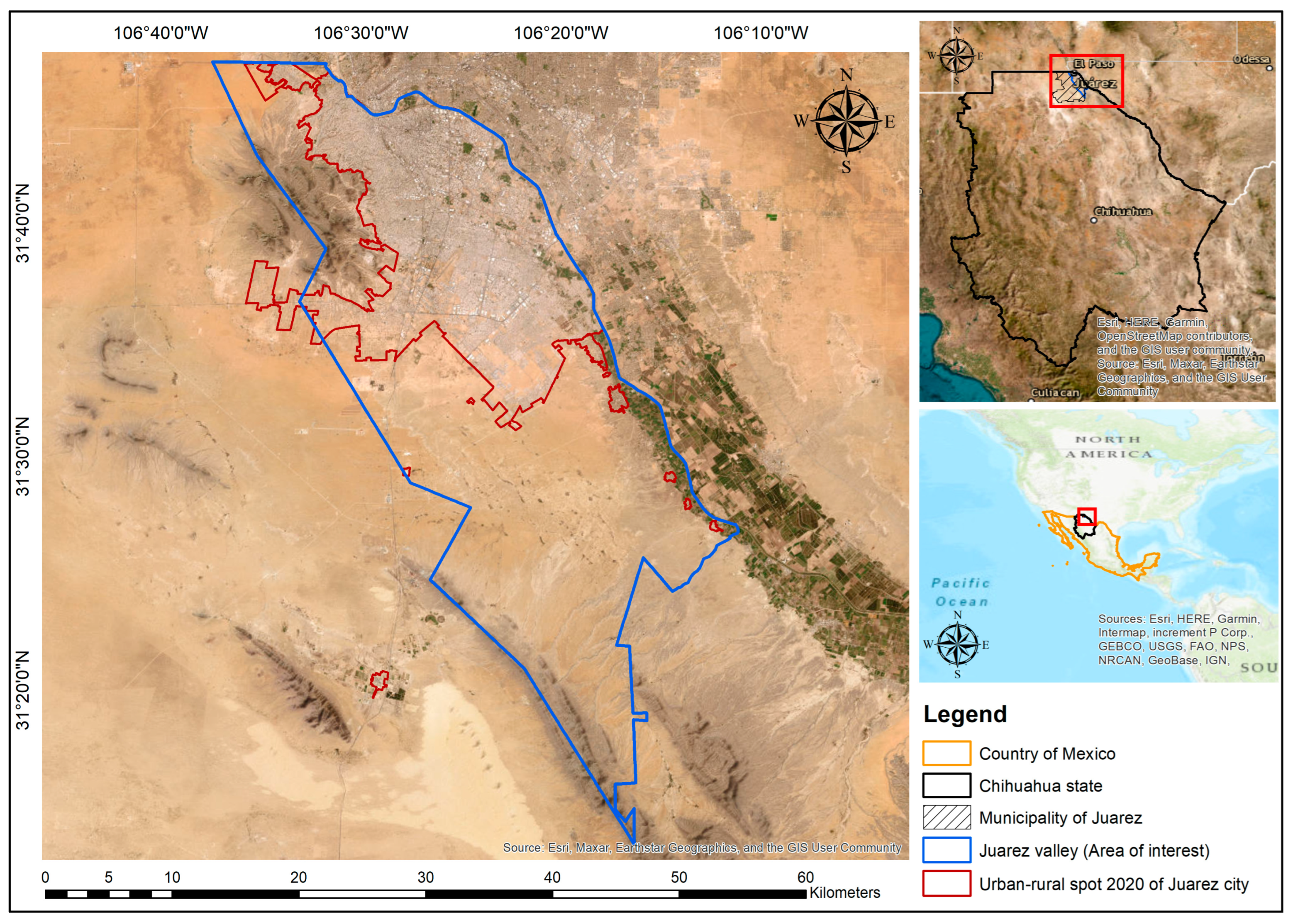
2.1. Study Area
The study area (AOI, area of interest) is located in the Juárez Valley, which is situated in the municipality of Juárez (
Figure 1) in the northern state of Chihuahua, Mexico. The area covers 962.08 km
2, with coordinates ranging from −106.623° to −106.180° longitude and 31.784° to 31.228° latitude [
16]. The altitude ranges from 1077 to 1817 m above sea level, with slopes ranging from 0° to 70° in small mountain ranges [
17]. The Juárez Valley is located on the Juárez aquifer (key no. 0833), with an area of 3386.44 km
2 [
16].
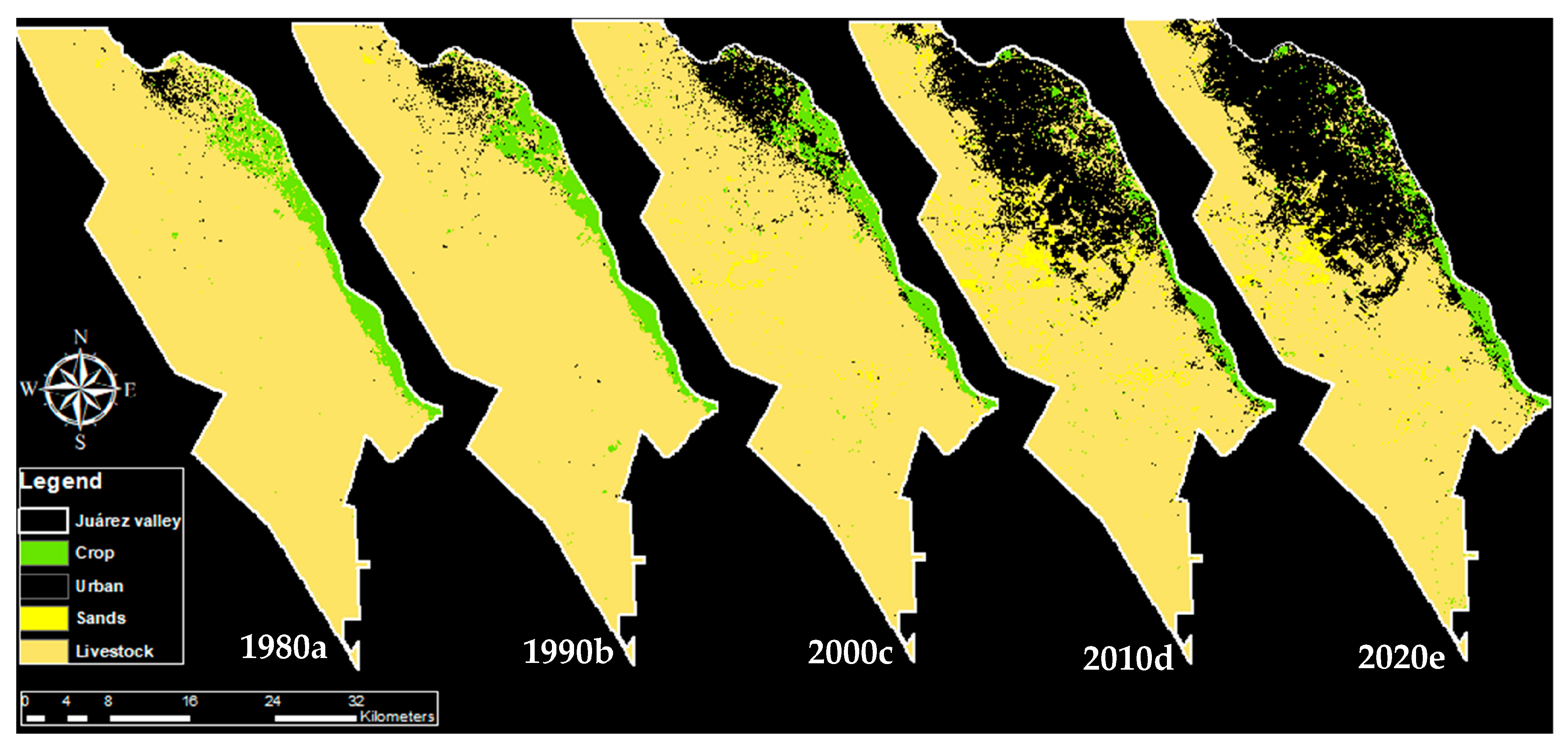
The main land uses and vegetation in the area are urban, agricultural, pasture, and shrub secondary vegetation. There is rainfed and irrigated agriculture [
18]. Cervantes and Montano [
19], in their book
El Valle de Juárez, mentioned that the main crops are alfalfa, sudan grass, pistachio, corn, wheat, cotton and sorghum, with regional environmental characteristics of average temperatures of 18.2 °C, a minimum of 7.5 °C and a maximum of 28.4 °C and an average annual precipitation of 265.3 mm and a population of 1,391,180 inhabitants as of 2015.
The processes used in this study (
Figure 2) utilized satellite images hosted in the Google Earth Engine™ (GEE) data catalog provided in cooperation with the United States Geological Survey (USGS). This cloud-based petabyte geomatics platform allows for the processing, analysis and visualization of imagery from various satellite platforms such as Landsat’s historical legacy platform of ETM+, TM and OLI/TIRS sensors [
20].
For the 1980s and 1990s, images were obtained for the Landsat 5 TM Collection Tier 1 mission calibrated for TOA (top of atmosphere) (LANDSAT/LT05/C02/T1_TOA courtesy of the U.S. Geological Survey) [
21]. For the 2000s and 2010s, Landsat 7 Collection 2 Tier 1 mission imagery calibrated to TOA (top of atmosphere) (LANDSAT/LE07/C02/T1_TOA courtesy of the U.S. Geological Survey) was used [
21]. The technical characteristics of these two platforms include a temporal resolution of 16 days, a multispectral band of 30 m, far infrared and thermal distances of 60 m and a Landsat 7 panchromatic band of 15 m, and their spectral ranges are from 0.45 to 2.35 μm [
22]. For the 2020s, images from the Landsat 8 OLI/TIRS Collection 2 Tier 1 mission calibrated for TOA (top of atmosphere) (LANDSAT/LC08/C02/T1_TOA courtesy of the U.S. Geological Survey) were used [
21]. The technical characteristics of this platform show a temporal resolution of 16 days operating under the same acquisition program as Landsat 5; the spatial resolution of the multispectral bands is 30 m, the panchromatic band of Landsat 8 is 15 m and its spectral ranges are from 0.443 to 1.375 nanometers [
22,
23].
Algorithms were developed on the GEE platform to analyze the multitemporal images. Date, boundary and cloud percentage filters were applied, and, subsequently, multispectral bands with spectral and spatial resolution were selected for the development of supervised and unsupervised classifications. Since the scenes available in the platform already have an atmospheric correction, this process was not applied. Date filters covering months with a lower percentage of cloud (<10%) were used next, and the boundaries (AOI) were loaded to the data warehouse and served as a mask file for extraction. Based on the filtered scenes, statistical reducers where the output is calculated per pixel were applied so that each pixel of the output was composed of the mean value of all images in the collection at that location (
Figure 3) [
20,
21,
22,
23,
24].
To obtain a multitemporal image, mosaics were generated. Images that did not comply with an acceptable percentage of cloudiness or coverage of the AOI of the studied regions were excluded, and cloud masking was applied using the quality band [
25] to generate better-quality images. For platforms with a panchromatic band, the HSV pansharpening technique [
26] was applied to increase the spatial resolution of the multispectral bands from 30 to 15 m.
For the Landsat 7 platform, the ETM+ sensor has an error from 2003 which causes banding or parallel lines and the absence of some information due to radiometric errors. To correct this drawback, interpolation and clustering techniques were applied following what was suggested by the USGS and EROS in 2004 [
27].
A classification based only on spectral variables can show confusion among objects with similar spectral responses. Spectral indices [
27,
28] of vegetation, soil, water or even indices based on RGB (red, green and blue) [
29] were used to discriminate pixels that could conflict in their spectral response. Among the indices used (
Table 1) to discriminate the pixels that could conflict in their spectral response, NDVI, GNDVI, EVI, AVI, SAVI, NDMI, MSI, GCI, BSI, NDWI, NDSI, NDSI and VARI were calculated by map algebra using the corresponding bands. The wavelength covered by each band per satellite platform varies; for example, it is not the same wavelength for Landsat 5 band 1 (blue) as for Landsat 8 band 1 (coastal aerosol). For the RGB indices, NGRDI, GLI and VDVI were calculated according to what Poley and McDermin mentioned [
30].
Physiographic variables were generated to support the classifier and indicate to the pixel its topographic or geographic position in the terrain [
31]. This information helps the classifier to recategorize a pixel in relation to its neighboring pixels by the value of its topographic position if it has the same spectral response and value in an index. A DEM (digital elevation model) obtained from the NASA-USGS (USGS/SRTMGL1_003 courtesy of the U.S. Geological Survey) was used for this purpose. This is a SRTM (shuttle radar topography mission) [
32] product with a spatial resolution of 30 m. The slopes and slope orientation variable were generated in degrees [
33].
As the first training and calibration variables, spectral separability was performed at the pixel level from an unmixing with the end members of each class (
Table 2). A transposed pseudo-inverse matrix was used to calculate the composite image for each class with the same number of bands. This technique is used in OBIA (object-based image analysis) [
34,
35].
To complement the OBIA processes, a segmentation of the physical and spectral characteristics representative of the objects that may contain the pixels was performed [
36]. The composite image was segmented into polygons of objects corresponding to their spectral and index values, shape and texture. Neighborhood groupings were integrated in this process, which are based on spatial contiguity and correspondence. This analysis determines if the behavior of a pixel is similar to its neighbor in its vertical, horizontal and vertex limits [
37,
38]. The integral efficiency analysis allows for accurate discrimination for the identification of objects and generation of training polygons based on statistics and geospatial behavior.
To train the classification algorithm, training points were generated by photointerpretation and the values corresponding to the spectral signatures that best represented each class or object. The identified classes were Crops, Urban, Sands and Livestock. The machine learning prediction algorithm of random forest [
39,
40] available in GEE was used. It was executed with a number of decision trees [
39] and the training points generated for each year and the variables or bands integrated in a single image.
The validation process consisted of comparing the results of the predictions or classifications against a set of independent data and calculating the kappa index that measures the level of agreement. This index allows us to know the degree to which the observers have certainty in their measurements or predictions [
41]. The results of the kappa index (Equation (1)) are obtained by subtracting a proposed theoretical contribution given to randomness (Equation (3)) from reliability. This yields a result that is less than the overall reliability (Equation (2)). For categorical mapping, a significant percentage of the random map should be correct for user agreement [
42].
where
Po = proportion of the area correctly classified (overall reliability), and
Pc = reliability resulting at random. Source: own elaboration based on Mas et al. [
42].
Table 3 shows the basic structure of a confusion matrix of size
n for the comparison of the georeferenced and map sites.
The results obtained for each period of each year were processed using a desktop GIS. The final layers were generated, and areas in hectares were calculated while isolating the land covers of interest. Formats for the classifications were prepared for their subsequent analysis in image processing software in the Land Use Change Modeler.
The LCM (Land Change Modeler) module was used to obtain the trends of land use change coverages, which allow for the mapping of transitions, permanences, losses and gains. The probability of change was calculated through Markov chains [
43,
44,
45] for the years 2025, 2030, 2050 and 2100 using 1980 as the base year and 2020 as the final and starting consecutive years to be predicted.
To generate the models, the input parameters were the results of each year with a normalized legend by ID and category. The first LCM result was calculated by overlapping the pixels of each category of the initial year against that of the end year. The units shown were indicated in pixel units, hectares or others.
From these options, cartographic results of losses, gains, persistence and transitions were constructed for each analyzed period and the historical period [
46,
47]. Finally, with the information stored in each of the models, tables of Markov chains or probability of future change were obtained [
48,
49].
2.2. Statistical Analysis
The GEE platform was used to call collections by their identifier corresponding to the Landsat 5, 7 and 8 platforms and filtered by dates and area of interest. For 1980, it was a collection from 22 August 1982 to 1 May 1985, depending on image availability and cloud percentage (<10%). The multispectral bands to be used were selected, and this process was repeated for the other platforms, modifying the date filter. For 1990, it was from 1 January to 31 December 1990. For 2000, 2010 and 2020, a mosaic was generated, and a statistical reducer was applied to the median.
The quality of the filtered images was improved by optimizing the value of the pixels through a masking operation, selecting the quality statistics band and a bit-by-bit operation [
50]. The HSV technique of pansharpening, used by Poveda et al. [
26], was applied to the platforms that had a panchromatic band of 15 m spatial resolution. The necessary bands to construct the spectral indices were selected, as indicated by Santos et al. [
28] and Roque [
29]. The equations of the University of Bonn portal were accessed and solved by means of an expression in map algebra. The necessary bands to construct the spectral indices were selected [
31], and slope variables in degrees and slope orientation [
33] were constructed using the SRTM DEM.
For the OBIA spectral separability analysis, the spectral bands of the image, indexes and physiographic variables were integrated into a single, multiband image according to Ela and Claire [
34] and Ramandhan et al. [
35]. The SNIC (simple non-iterative clustering) algorithm was used for segmentation, and a reducer was applied to the clustering band [
36,
37,
38].
In the final stage of the random forest (RF) classifier, the arguments from Phan et al. [
39] and Amini et al. [
40] were incorporated. An image composed of the bands obtained by unmixing, segmentation, physiographic and multispectral bands, their respective labels of each band with 500 decision trees [
39] and the series of training points generated from a base sampling taken from Mas et al. [
42] were used. This is a hybrid method combining systematic and clustering methods (MH). Ground truth points were obtained through photointerpretation and expert knowledge, representing each category of land use and vegetation analyzed.
The land use classifications for each year were validated using the kappa index and INEGI cartography scale 1:250,000, as indicated by Mas et al. [
42]. Values were extracted from all series that were constant in their categories between 1980 and 2020. The sampling used the MH method, generating a 2000 × 2000 m grid with points created on each line at a distance of 15 m (133 points), to which points by clusters were added [
42]. These were created within each polygon of the grid, where the minimum distance between them or the area of influence was 500 m so that each category or class within the quadrant had the same probability of being evaluated.
To run the LCM, classifications were spatially adjusted by resampling, ensuring that the spatial configuration was homogeneous in pixel size and number of columns and rows These were converted to ASCCI format for export to Terrset™ software and added to the soil change modeling processes in the LCM module, as mentioned by Anand and Ainam [
43], Hamad et al. [
44] and Sundara et al. [
45]. Models were run for each decade between 1980 and 2020, and predictions of changes for the dates of 2025, 2030, 2050 and 2100 were obtained, feeding the processes of gains, losses and transitions [
46,
47] to obtain the net contributions through Markov chains [
48,
49].


 ,
, 


