Article

Trade-Off Analyses of Food Loss and Waste Reduction and Greenhouse Gas Emissions in Food Supply Chains

Wageningen Food & Biobased Research, Wageningen University & Research, 6708 WG Wageningen, The Netherlands
*
Author to whom correspondence should be addressed.
Sustainability 2023, 15(11), 8531; https://doi.org/10.3390/su15118531
Submission received: 28 February 2023 / Revised: 28 April 2023 / Accepted: 9 May 2023 / Published: 24 May 2023
(This article belongs to the Special Issue Sustainability in Agri-Food Supply Chain: From Farm to Fork)

Abstract

:
Food losses and waste (FLW) reduction and mitigating climate impact in food chains are priorities in achieving sustainable development goals. However, many FLW-reducing interventions induce additional greenhouse gas (GHG) emissions, for example, from energy, fuel, or packaging. The net effect of such interventions (expressed in GHG emissions per unit of food available for consumption) is not obvious, as is illustrated in a number of case studies. We recommend that in the decision to take on FLW-reducing interventions, the trade-offs on sustainability impacts (such as GHG emissions) are taken into consideration. Since FLW induce demand and extra operations in all stages along a supply chain, adequate representation of cumulative GHG emissions along the production and supply chain, including ‘hidden parts’ of the chain, is required, which is challenging in full LCA studies. As a workaround, the case studies in this paper are based on a generic tool, the Agro-Chain greenhouse gas Emission (ACE) calculator that includes metrics and data for common food product categories and supply chain typologies. The calculator represents the structure of a generic (fresh food) supply chain and offers data sets for, amongst others, crop GHG emission factors and FLW in different stages of the production and distribution chain. Through scenario calculations with different chain parameters (describing pre and post-intervention scenarios), the net effects of an intervention on GHG emissions and FLW per unit of food sold to the consumer can be compared with little effort. In the case studies, interventions at the production stage as well as in post-harvest operations, are analyzed. Results show that post-harvest activities (especially FLW) contribute substantially to the carbon footprint of supplied food products. The FLW-reducing interventions are considered to induce additional GHG emissions. In most case studies, FLW-reducing interventions lower total GHG associated with a unit of food supplied to a client or consumer. However, in one case study, the extra emissions due to the intervention were higher than the prevented emission from lowering food losses. Consequently, in the latter case, the intervention is not an effective GHG emission reduction intervention.

1. Introduction

Food losses and wastes (FLW) significantly impair food security. Moreover, substantial environmental impacts are coupled with the production of the lost produce. Reducing FLW is considered an effective measure for both fulfilling food demand and reducing the associated environmental impacts since the greenhouse gas (GHG) emissions associated with the generation of extra food to compensate for the losses can be avoided. However, most FLW-reducing interventions will not only lower environmental impact per unit product available for consumption but also induce extra emissions (amongst others through energy, fuel, and packaging material use). Estimating net trade-offs of FLW-reducing interventions and emissions is far from obvious.
In food supply chains, a large fraction of the total GHG emissions are related to agricultural production [1]. Total GHG emissions due to agriculture, forestry, and other land use are estimated at around 12 Gt CO2-eq. per year [2]. Post-harvest operations, such as long-distance transport, processing, packaging, and refrigeration, add another 2.5 Gt and households 1 Gt CO2-eq. ([3], based on data from [4,5,6]). Food losses affect total GHG emissions because they induce extra crop production and post-harvest emissions up to the point where the product is lost. Ref. [7] estimates that 8–10% of global GHG emissions are associated with food that is not consumed
The ambition to reduce FLW (currently estimated at 30% of all food produced in the world for human consumption [8]) by half in 2030 (in line with the United Nations’ Sustainable Development Goals target 12.3 [9]) is supported by an increasing number of stakeholders in governments and throughout food supply and consumption chains. The realization of this ambition corresponds to the reduction of agricultural production by one-sixth, currently produced only to be lost. Since the loss percentages are lower for animal products (with relatively high GHG emission intensities) than staple crops and fruit and vegetables [10], GHG reductions through reduced FLW will be somewhat lower than one-sixth of the total GHG emissions related to food, but still very substantial.
FLW-reducing interventions such as packaging, refrigeration, and intensified transportation will induce extra emissions. Still, many, see, e.g., [11], estimate that “halving food loss and waste would reduce environmental pressures by 6–16% compared with the baseline projection”. However, additional emissions induced by the FLW-reducing interventions were not considered in those estimates. In this paper, we—through a number of case analyses—show that reducing FLW does not automatically result in a net reduction of GHG emissions; we argue that situational analysis is essential to select interventions with a net positive trade-off between FLW and GHG emission reduction.
The question is how to estimate the net effects for a specific product chain, thus, how to compare a conventional situation to a supposedly improved situation in numerous distinct case studies. For that, we propose the Agro-Chain greenhouse gas Emissions (ACE) calculator. That calculator accounts for the emissions generated during the entire production cycle of the product and corrects for losses at each operation, as is commonly done in life cycle analysis. Compared to common tools for life cycle analysis, which require significant resources and time and where data collection is considered a major challenge [12,13,14], the ACE calculator is simpler and less laborious and, therefore, more suitable for rapid estimation of the net effect of an intervention. The tool is provided with default parameter values for all operations along a value chain so that the user can limit data specification to the operations (or differences between scenarios) in the scope of the study. The ‘default’ values are derived from review papers and are considered typical/representative of the ‘unknown’ chain parts. By integrated calculation of effects of loss percentages as well as emissions related to energy use, fuel use, and (packaging) material use, the tool supports the analysis of GHG emission effects of loss-reducing interventions through comparisons of reference situations with intervention scenarios.
In order to estimate the carbon footprint per unit of supplied food, the ACE calculator adopts a product approach, such as the Cool Farm Tool [15], which is fundamentally different from methods that support the assessment of carbon footprints of regional agro-food systems (such as the EX-Ante Carbon-balance Tool EX-ACT [16]). The scope of the ACE calculator is limited to the post-harvest chain; for crop production, default/typical values are provided (specified to crop categories and seven global regions). For more dedicated studies, specific values for crop GHG emission intensity can be inserted in the tool; such more specific values may be derived from other calculators for crop production GHG emissions, such as the Cool Farm Tool or the Food Loss and Waste Value Calculator (Quantis [17]).
One of the major challenges of analyzing the post-harvest chain is collecting data on food losses. In many practical situations, only a limited set of data or estimates are available. In order to facilitate quantitative analysis, the calculator is supplemented with a complete set of FLW estimates per chain stage (averages at product category level and specified for typical post-harvest chain configurations, differentiated for seven global regions).
For analyzing trade-offs between FLW and GHG emissions, it is essential to create insight into the distribution of GHG emissions of all operations along the chain and to compare different scenarios (i.e., without and with FLW-reducing interventions). These functionalities are provided in the ACE calculator.
The method (including the ACE calculator) is explained in the following chapter. Section 3 outlines the process of using the ACE calculator to estimate the effects of FLW-reducing interventions. Section 4 shows results from various case studies; these illustrate that the net benefit of expected ‘climate smart’ measures may turn out positive or negative, dependent on the specific situation.

2. Method: Agro-Chain Greenhouse Gas Emissions (ACE) Calculator

2.1. Problem Statement: Assessing GHG Emissions of Food Supply

Assessing GHG emissions of food supply requires a specification of operations, inputs, and outputs (including losses) and associated GHG emission effects. In order to quantify the effects of FLW along the chain, cumulative GHG emissions associated with the lost product must be known. Altogether the following information is required:
  • A specification of the food supply chain, including geographic locations of production and final market, transportation distances and modalities, use of energy (for cooling and other operations) and fuels, other inputs (including packaging material), FLW percentage per chain stage, and FLW management practices. These parameters are case-specific and must be provided per case study;
    In scenario studies on FLW-reducing interventions, the inputs (such as packaging material used and refrigeration energy use) or logistic parameters may vary between the scenarios;
  • GHG emission intensities of inputs and residue management: crop production, electricity, fuels, packaging materials (plastics, steel, aluminum, glass, …), and loss/waste management options.
In most situations, primary data values for specific values (such as crop GHG emission intensities and FLW factors in different stages of the supply chain) are lacking.

2.2. Explanation of the Agro-Chain Greenhouse Gas Emissions (ACE) Calculator

The ACE calculator describes all activities (with inputs and losses per operation) along the supply chain, starting with the farm (crop GHG intensity) and ending at the point of sale (for which the product’s carbon footprint is calculated).
In order to relieve the data demand, a workaround has been created by providing a large set of secondary data:
  • Crop GHG emission intensities
    • Average/typical values are provided for all crop categories (FAOSTAT [18] coding), detailed per global geographical region: Europe; North America and Oceania; Industrialized Asia; Sub-Saharan Africa; North Africa, West and Central Asia; South and Southeast Asia; and Latin America. These datasets are derived from the review by [1];
    • More specific values for a country or specific farming situation (e.g., smallholder production) are derived from dedicated studies and from [18] for rice and animal products.
  • Loss factors along supply chains
    • Average/typical values are provided per crop category, specified per the aforementioned global region, again derived from the review by [1];
    • For situation-specific analysis, more dedicated data may be required. More specific data for a small number of situations is given, but it is recommended to gather more specific information from other sources. Good examples of inventories that aggregate findings from diverse studies include the African Post-harvest Losses Information System APHLIS [19] and the Post-Harvest Loss Information System SIPPOC [20].
  • Typical GHG emission effects of FLW management options vary from landfilling to biogas production (derived from [21,22]);
  • Typical GHG emission intensities for transportation modalities: since often the emission standard of the actual vehicle used in a shipment is not known, average GHG emission intensities are recommended. These are specified for diverse sizes of road vehicles (from small vans to large trucks), bulk and containerized sea transport, and continental and intercontinental air freight. The GHG emission intensities were largely derived from [23,24];
  • Packaging materials: typical GHG emission intensities are provided for paper/carton [25,26], plastics [25,27], glass [28,29], steel [28,30,31,32], and aluminum [28,33,34];
  • Electricity: for a large number of countries (average), GHG emission factors are provided in the tool (GHG emissions associated with production [35,36,37] and transmission and distribution [38]). In addition, typical GHG emission factors are provided for a number of renewable energy sources [39,40];
  • Fuels: well-to-wheel GHG emission factors are included [28] (the actual well-to-wheel emission factor may vary slightly among countries/regions, but the differences are relatively small—less than 5%—and therefore neglected).
The actual values can be examined (and optionally updated) in datasheets embedded with the calculator. In order to accommodate scenario studies, some of these parameters may be overruled by case-specific values (Table 1) in the ACE calculator worksheet.
The minimum input required from the user is a specification of the product and chain configuration:
  • Geographic region and country of production and delivery;
  • Crop;
  • Transportation distances and modalities;
  • Packaging materials used;
  • Electricity use: the actual electricity use per unit material is material/process/situation-specific and, therefore, must be specified by the user. A provision is included for refrigerated storage because it is broadly adopted in food supply chains; if electricity use for refrigerated storage is not specified, a default electricity use of 1 kWh per ton per day is suggested (estimated from [41]).
Table 1. Uses of the ACE calculator and data source per use type.
Aggregation level of dataAverages for crop category per geographical regionSpecific data for a dedicated crop, chain configuration and/or specific countrySpecifically defined unit operations along the chain
ExampleRoots and Tubers, Sub-Saharan AfricaCassava Sub-Saharan AfricaCassava MozambiquePotato KenyaCassava Mozambique, traditional processing Cassava Mozambique, mobile processing unit
Specific data source crop GHG emission factorAverage data (we used values from [1])Reference data sets such as FAO emissions database [18].
Dedicated literature source (country/chain study); see, e.g., [42,43].
Calculated value through an external calculator (e.g., Cool Farm Tool [15] or the Quantis Food Loss and Waste Value Calculator [17].
Dedicated literature source (country/chain study).
Calculated value through an external calculator
Specific data source FLW factors along the chainAverage data (we used values from [1])Reference data sets like APHLIS [19] and SIPPOC [20].
Dedicated literature source.
Direct measurements.
Dedicated literature source.
Expert estimate of the effect of the intervention on FLW.
Direct measurements.
Typical useEstimating average FLW and food supply GHG emissions at the food category levelAssessing/comparing different supply chain types or crop types that fulfill a nutritional need. Assessing/comparing net effects of different technology options.
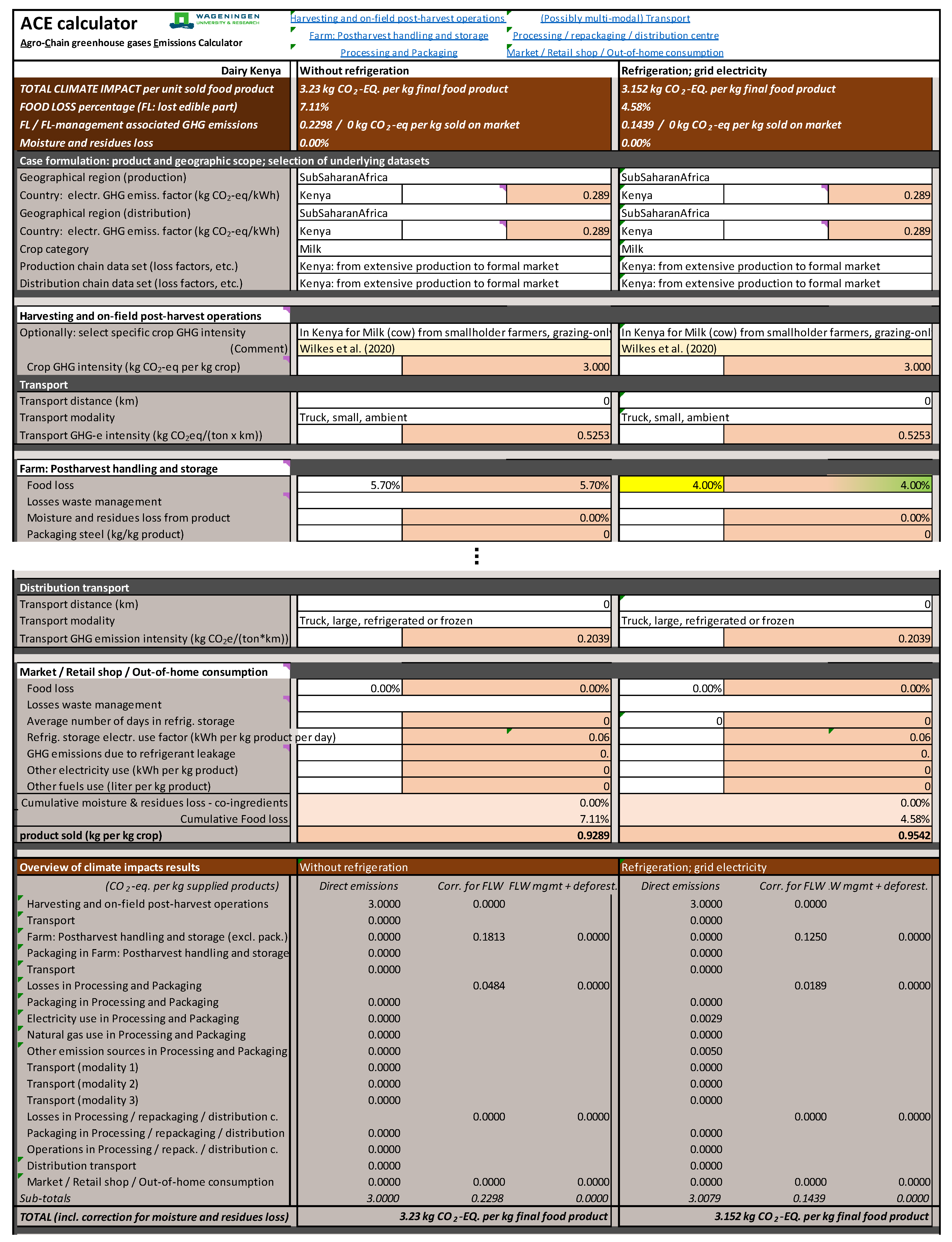
The ACE calculator provides fields for filling in the case-specific parameters and for optimally overwriting default values, as well as a summary table of GHG emissions due to different operations along the supply chain (Figure 1). The total calculated carbon footprint per unit product delivered is presented on top of the screen, whereas at the bottom of the user-interface, contributions of emissions are summarized.
Figure 1. Screenshots of parts of the ACE calculator user interface. Comparison of two scenarios for dairy supply chain configuration in Kenya. For convenience, differences between scenarios are indicated by highlighted cell colours: yellow, green or red (red not applicable in this figure) [44].
Sustainability 15 08531 g001

2.3. Conceptual Comparison with Existing Approaches

A comparison of various tools for FLW/GHG calculations (including a draft version of the ACE calculator) has been presented by WRI/Food Loss and Waste Protocol [45]. The scopes of listed calculators vary a lot, typically:
  • Estimating environmental impact per unit lost food: effects of destinations, including waste management options (EPA Waste Reduction Model);
  • Estimating environmental impact per unit lost food, including impacts of their agricultural production and effect of destinations of the lost product (for distinct food types: FLW Value Calculator, for distinct food basket types: ReFED US Impact Calculator);
  • Estimating impacts of crop–livestock production, including first-level processing (storage, packaging, grading) and transport (Cool Farm Tool);
  • Estimating GHG emissions of purchased foods, based on typical GHG emission intensities of food products, not specified to origin (Cool Food Calculator).
Another renowned tool not listed by WRI is FAO’s EX-ACT. This provides ex ante estimates of the net balance of GHG emissions, expressed in tCO2-e, emitted or sequestered following the realization of a project. Connected to that, the add-on EX-ACT VC can be used for estimating emissions of collection and delivery transport, processing energy, and packaging material used. Losses along the value chain are represented through the total GHG emissions per unit supplied product.
Most are aimed at raising awareness of the impacts of FLW and thriving to more sustainable waste management and higher valorization. Most calculators use typical/average GHG intensity factors for crops and crop mixes.
From the above tools, the functionality of EX-ACT VC seems most suited for analyzing trade-offs between food loss and waste reduction, and greenhouse gas emissions in food supply chains. However, the level of the detailed description of value chains is only suited for local/regional/national value chains (in line with the purpose of the EX-ACT tool: regional development plans). Furthermore, the calculations EX-ACT VC use fixed emission factors for inputs are used (most of them based on dated studies); no means are provided to update these in the tool.
Next to the dedicated tools, general LCA software may be used for the assessments. This is, however, in general quite laborious unless LCA models for similar chain configurations are available.
It is concluded that the ACE calculator provides a valuable addition to existing tools, uniquely suited for estimating GHG emissions in specific food supply chains and trade-offs between FLW and GHG interventions.

2.4. Limitations of the ACE Calculator

The scope of the ACE calculator is limited to the post-harvest chain and activities described above.
The accuracy of the result depends on the validity of the data. For instance, typical GHG emission factors are used for transportation (differentiating amongst others different road transport types, such as vans, small, medium, and large size trucks, sea bulk transport, sea container transport, and continental and intercontinental airfreight). However, the GHG emission factors are based on average capacity utilization factors. Likewise, the provided crop GHG emission intensities and loss factors along supply chains are average/typical values. Consequently, results generated by the ACE calculator are considered estimates. For LCA reporting, the adequacy of the data should be validated (and, as indicated, updated values may be inserted in the calculator).

3. Analyzing Climate Impact Effects of Interventions in Supply Chains

FLW-reducing measures include technical, logistical, or marketing interventions. Technical interventions are often shelf-life-extending measures (refrigeration, packaging, or other preservation methods). Logistical or marketing interventions may lead to supply chain lead time reduction, reduction of demand variance, etc. [46]. Each intervention will have multiple direct and indirect effects affecting FLW and GHG emissions. There are direct effects, such as emissions related to energy and packaging material used. Indirect effects are, for instance, related to increased tare weight (packaging) in transport, altered average storage durations (influencing energy use in refrigerated storage), and loss percentages which will be affected and/or shifted to other stages along the supply chain, etc. Trade-offs between energy and material use, FLW, and GHG emissions can be analyzed by modeling the reference situation and alternative supply chain configurations. Think of interventions such as:
  • Applying refrigeration or lowering the storage temperature in the chain (which may result in extended retail shelf life and reduction of FLW but will lead to an increase in energy use);
  • Applying protective packaging (which may lead to a reduction of losses, but at the cost of using packaging materials);
  • Transfer processing to a location near the crop production (this may lead to a reduction of transportation, but at the cost of increasing energy use: a regional, small-scale facility generally has lower energetic efficiency than a large-scale centralized processing facility).
For each scenario, the parameters such as transportation distances, packaging materials, storage durations, and FLW percentages per chain stage must be estimated (Table 1).
Quantitatively estimating the net effects of FLW-reducing interventions on GHG emissions requires an understanding of product quality decay, logistics processes, and demand. Quantification based on collecting primary data is one option. This requires data for the reference and new configuration where all conditions except for the intervention are comparable. This will only be possible in exceptional situations. Estimating effects from secondary data is another option, for instance, by deriving effects from comparable interventions in analogous systems (measured or described in the literature) or by making use of expert estimates or model-wise estimation of the effects. The latter option will require quantitative models (for product quality decay/shelf life, quantifying effects of the intervention on shelf life), logistic models (quantifying effects on transportation quantities, distances, and efficiency), and/or market models (quantifying, for instance, effects of supply characteristics and shelf life on loss percentage). An adequate methodology is described by [46].

4. Results—Case Studies on Effects of FLW Reductions on GHG Emissions

Below, six case studies are presented, in which the mitigation effect of adapting post-harvest operations on losses and GHG emissions are estimated, highlighting the importance of trade-offs and achieving net emissions reduction.
In these case studies, it is assumed that all secondary data presented in Chapter 2 apply; exceptions are mentioned in the case study explanations. Consequently, the specific results generated can be considered typical results.
All data and results from the case studies are presented in the Supplementary Material.

4.1. Case Study: Cooling in Milk Collection Chains in Kenya

Milk is an important agricultural product category in Kenya in terms of value creation by farmers and as well as for nutritional contribution to the average diet. Milk produced in rural areas is commonly consumed by families and (freshly) traded in the vicinity of the farmers. Losses in such chains are quite limited: [6] reports 5.7% losses at the farm (mainly evening milk), 1.5% loss at trader collection centers (without cooling), and 0.6% at co-operatives (with cooling facilities). Similar values are presented by [47,48]. An often suggested intervention is the introduction of small-scale refrigerators at the farmer (group) level, with a typical capacity of 100 to 200 liters of milk connected to the electricity grid or equipped with solar panels with a cold buffer. Results for the reference situation (5.7% losses at the farm, 1.5% at the collection center) and with the intervention (assuming that the losses in farming are reduced to 4%, 0.6% loss at the collection point) are given in Figure 2. In these analyses, the carbon footprint of milk was assumed to be 3 kg CO2-eq. per kg milk [44], GHG emissions related to refrigerator production at 0.005 kg CO2-eq. per kg milk (estimated from [49]), solar panel production at 0.005 kg CO2-eq. per kg milk (estimated from [40]), whereas the refrigerator’s electricity use (when connected to the electricity grid) is estimated at 0.01 kWh per kg milk.
The above results show that GHG induced by cooling (either equipped with a solar panel or using electricity from the grid) is substantially smaller than the GHG savings by FLW reduction. This underpins that, although the intervention is often not yet economically feasible, cold chain development is essential for projects that aim at increasing milk production in rural areas for urban markets, especially since the local surplus of evening milk will increase significantly then.

4.2. Case Study: Lowering the Storage Temperature for Bovine Meat in The Netherlands

Because of the high GHG emission intensity of beef, losses in the value chain induce substantial associated GHG emissions. One intervention (already current practice in the Netherlands) is lowering the maximum refrigerated storage temperature from 7 to 4 °C. This results in extended shelf life and consequently reduced FLW and FLW-associated GHG emissions in retail, but increases refrigeration energy use and energy-induced GHG emissions.
Through the intervention, the total maximum shelf life is extended by approximately three days [46]. Model simulations of a typical retail and buying profile predict an average keeping period (and thus refrigeration energy use) increase of 5 h. Furthermore, the energy use per day is increased because of the lower temperature (estimated at +50%). Analysis with Tromp et al.’s model shows an average loss reduction on the shelf of about 2%.
Specific parameter values for the scenarios are listed in Table 2 and Table 3.
Carbon footprint results per kg product sold to the consumer for both scenarios are summarized in Figure 3. Apparently, the GHG emissions savings through FLW reduction are much higher than the effects of higher energy use for cooling.

4.3. Case Study: Lowering the Keeping Temperature for Packaged Fresh-Cut Vegetables in The Netherlands

Here the same intervention as for beef is tested for cut vegetables. Factors deviating from the beef case are specified in Table 4.
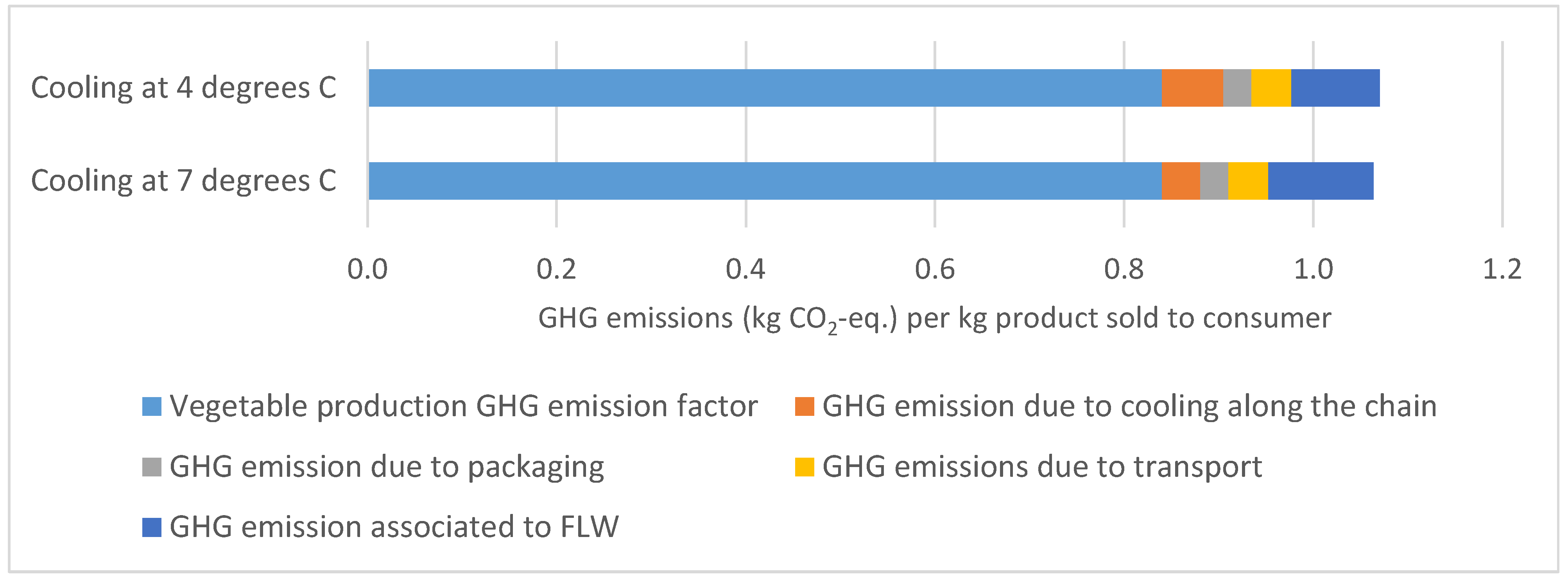
The substantially smaller carbon footprint of vegetable production compared to beef production is reflected in the total GHG emissions per kg sold in retail. However, because of the smaller carbon footprint of the product, the loss reduction results in small GHG emission reductions (in absolute terms), whereas the extra energy used for cooling is equal to that in the beef case study. In total, in this comparison, the intervention induces more GHG emissions compared to the reference situation (Figure 4).

4.4. Case Study: Effects of Modified Atmosphere Packaging in Melon Shipping from Honduras to UK

Intercontinental fruit transport is mostly done through refrigerated reefer containers. Modern packaging solutions (modified atmosphere packaging) result in the reduction of product losses compared to the common situation (without packaging). Specific parameters for this case study are given in Table 5.
Results for both scenarios are presented in Figure 5. Apparently, the GHG emission saving by reducing the FLW is higher than the GHG emissions induced by plastic use.

4.5. Case Study: Tomato Varieties for Traditional Smallholder Chains in India
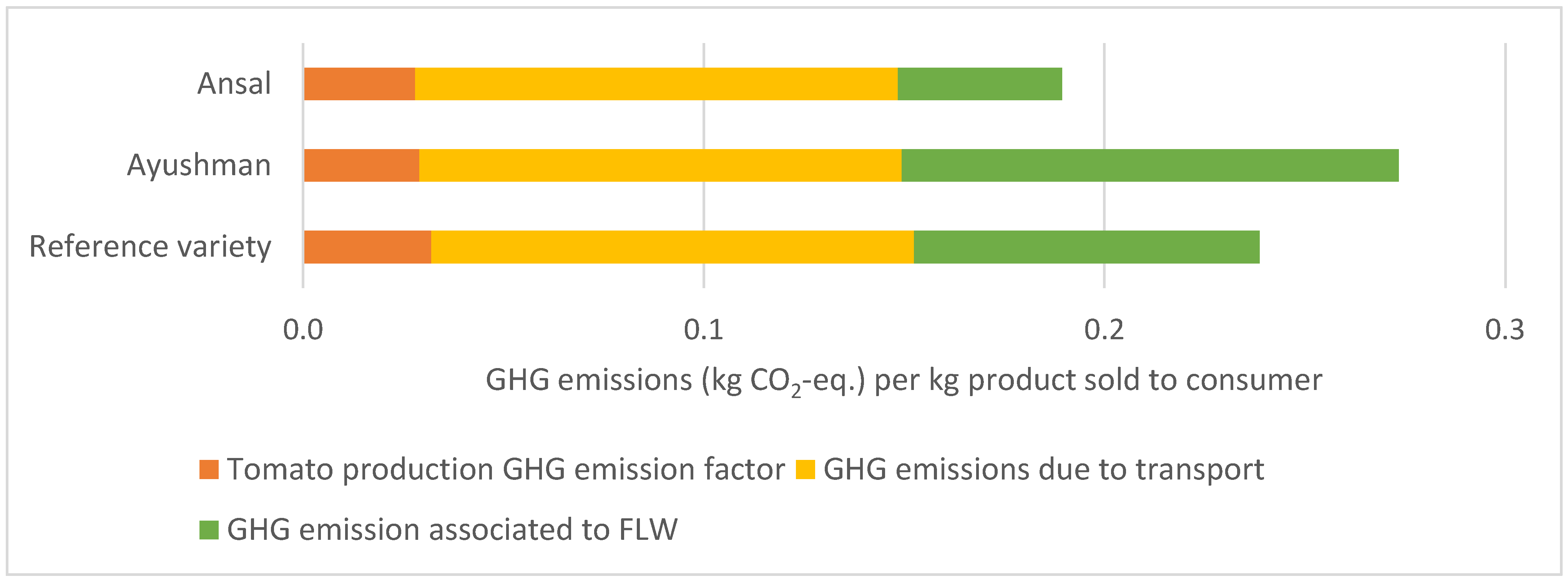
Different strategies can be applied in crop breeding to improve food security and reduce environmental impact, for instance, through increasing crop yield or improving products’ shelf life (in the challenging conditions of low-tech post-harvest chains). Bayer has recently developed different hybrid tomato varieties according to these strategies (see also [51]): Ayushman with increased yield and Ansal with improved shelf life. Specific data (provided by Bayer) are given in the following table.
Results (Figure 6) reveal that the increased yield of the Ayushman variety is annihilated by increased sensitivity to loss in the post-harvest chain. That variety is vulnerable to damage in long-distance transport and more suitable for local markets. The improved shelf life of Ansal is a strong success factor for serving remote markets.
Figure 6. Climate impact of tomato (kg CO2-eq. per kg sold to consumer) for scenarios detailed in Table 6.
Sustainability 15 08531 g006

4.6. Case Study: Supplying Dragon Fruit from Vietnam to Europe

Novel tropical fruits such as dragon fruit are transported to western markets through air transportation (most common, with high GHG emissions due to transport) and sea transportation (refrigerated reefer containers, with relatively low GHG emissions, but less frequently applied because of unreliable quality of the fruit and high losses because of product quality decay). In an expert consultation, a set of interventions was proposed—improve growing techniques and handling to increase the quality of the fruits combined with cold chain (pre-cooling quickly after picking and closed cold chain)—that is expected to eliminate the hotspots [52]. The intervention will prevent rapid quality decay during the first days after harvest and consequently significantly extend total shelf life under refrigerated conditions, resulting in significantly lowered rejects after (reefer) sea transport.
The outcomes of the scenario study (Table 7) highlight the hotspots of GHG emissions in air transportation and food losses in the case of sea transport. Furthermore, these demonstrate that the dramatic high losses in the case of sea transportation result in comparable GHG emissions as air transportation does; consequently, the common routes through air and sea result in more or less comparable climate impact per unit product on the end market. However, the air scenario does not allow for scaling as the cost price for the dragon fruit is simply too high to increase market shares. Next to that, most European retailers try to avoid airfreight as they aim for a decrease in their carbon footprint. The intervention results in significantly lower GHG emissions per unit product on the end market.

5. Conclusions

Reducing FLW can significantly contribute to reducing food-related GHG emissions. However, many FLW-reducing interventions will induce additional emissions. These trade-offs make the selection of FLW-reducing interventions a complicated decision, with the risk that FLW reduction is postponed in the absence of an evidently effective solution. Therefore it is imperative to enable rapid assessment of the trade-offs in the selection of FLW-reducing interventions. Based on (estimated) net effects, interventions that synergistically contribute to reducing FLW and reducing food-supply-related GHG emissions can be prioritized.
Through a number of case studies, we have shown that not only agricultural production but also processes in the post-harvest chain add significant GHG emissions to the food supply. It is demonstrated that FLW-reducing interventions may add substantial extra emissions. In most case studies reducing FLW results in a net reduction of GHG emissions per unit of supplied food. In one case study, however, the extra emissions due to the intervention are higher than the prevented emission from lowering FLW; the net effect is an increase of GHG emission per unit of supplied food. Hence, it is concluded that reducing FLW does not straightforwardly result in reducing GHG emissions.
With an eye on the high urgency of GHG emission mitigation and improving food security solutions, the synergy between FLW reduction and GHG emission reduction should be prioritized. Therefore it is recommended, before actually implementing FLW-reducing interventions, to analyze the trade-offs with GHG emissions.
A tool that supports such analysis at minimum efforts was introduced for that purpose in this paper: the ACE calculator. This calculator supports the identification of GHG emission hotspots along a chain (pointing to activities that are most interesting for interventions). Furthermore, it supports the comparison of GHG emissions for different food supply chain scenarios. Such comparisons support the assessment of net GHG emission effects of FLW interventions. This calculator combines metrics for estimating climate impacts along a food chain with secondary data, facilitating a quick assessment. A complete set of secondary data (including crops GHG emission factors aggregated at the product category level and FLW estimates per chain stage) is provided, aggregated at the product category level; all data are differentiated for seven global regions. After prioritizing an intervention based on those secondary data, more accurate estimates of the effects can also be made with the calculator by inserting (primary or more specific applicable secondary) data. The tool is highly suitable for assessing net GHG emission effects of FLW-reducing interventions: comparing different chain configurations, each with adequate FLW estimates.
The ACE calculator supports prioritizing climate-smart FLW reduction interventions. The approach can support the identification of GHG emission hotspots (as potential priorities for GHG emission mitigation) and the assessment of the actual mitigation effects of interventions. This is expected to help overcome decision-making paralysis.
We hope that making this tool publicly available will contribute to the actual adoption of solutions that result in GHG emission mitigation.
In the development of this tool, some essential data lacking became clear. Although there is an increasing set of crop carbon footprint data, the high diversity of crops, production regions, production conditions, and agricultural management practices are not covered. We aspire that sizeable new data will be generated in dedicated studies.

Supplementary Materials

The data presented in the case studies are available in https://www.mdpi.com/article/10.3390/su15118531/s1. The ACE calculator can be downloaded at https://www.wur.nl/nl/project/A-new-approach-towards-Food-Loss-and-Waste-including-Greenhouse-Gas-Emissions.htm (accessed on 25 August 2020).

Author Contributions

Methodology, J.B.; data collection, X.G.; case study management, H.A.; writing, J.B. All authors have read and agreed to the published version of the manuscript.

Funding

Support for this study was provided through the CGIAR Research Program on Climate Change, Agriculture and Food Security (CCAFS) and CGIAR Research Program Mitigate+: Initiative for Low-Emission Food Systems. We would like to thank all funders who supported this research through their contributions to the CGIAR Trust Fund. This work was furthermore supported by the US Foundation for Food and Agriculture Research under award number—Grant ID: DFs-18-0000000008 and by the Rockefeller Foundation under award number 2018 FOD 004.

Data Availability Statement

All generated data are provided in the Supplementary Material.

Conflicts of Interest

The authors declare no conflict of interest. The content of this paper is solely the responsibility of the authors and does not necessarily represent the official views of the sponsors or any other party.

References

  1. Porter, S.D.; Reay, D.S.; Higgins, P.; Bomberg, E. A half-century of production-phase greenhouse gas emissions from food loss & waste in the global food supply chain. Sci. Total Environ. 2016, 571, 721–729. [Google Scholar] [PubMed]
  2. IPCC. Climate Change 2014: Mitigation of Climate Change. Contribution of Working Group III to the Fifth Assessment Report of the Intergovernmental Panel on Climate Change; Edenhofer, O.R., Pichs-Madruga, Y., Sokona, E., Farahani, S., Kadner, K., Seyboth, A., Adler, I., Baum, S., Brunner, P., Eickemeier, B., et al., Eds.; Cambridge University Press: Cambridge, UK; New York, NY, USA, 2014. [Google Scholar]
  3. I4CE; Rogissart, L.; Foucherot, C.; Bellassen, V. Food Policies and Climate: A Literature Review, Institute for Climate Economics. 2019. Available online: https://www.i4ce.org/wp-core/wp-content/uploads/2019/03/0306-I4CE2984-PolitiquesAlimentairesEtClimat-Etude24p-VA_V2.pdf (accessed on 25 August 2020).
  4. Vermeulen, S.J.; Campbell, B.M.; Ingram, J.S.I. Climate Change and Food Systems. Annu. Rev. Environ. Resour. 2012, 37, 195–222. [Google Scholar] [CrossRef]
  5. Poore, J.; Nemecek, T. Reducing Food’s Environmental Impacts through Producers and Consumers. Science 2018, 360, 987–992. [Google Scholar] [CrossRef] [PubMed]
  6. FAO. Food Wastage Footprint Full-Cost Accounting: Final Report; FAO: Rome, Italy, 2014. [Google Scholar]
  7. UNEP. Food Waste Index Report 2021; United Nations Environment Programme: Nairobi, Kenya, 2021. [Google Scholar]
  8. Guo, X.; Broeze, J.; Groot, J.; Axmann, H.; Vollebregt, M. A global hotspot analysis on food loss & waste and associated greenhouse gas emissions. Sustainability 2020, 12, 7488. [Google Scholar]
  9. United Nations General Assembly. Resolution Adopted by the General Assembly on 25 September 2015. 70/1 Transforming Our World: The 2030 Agenda for Sustainable Development; United Nations General Assembly: New York, NY, USA, 2015. [Google Scholar]
  10. Gustavsson, J.; Cederberg, C.; Sonesson, U.; Otterdijk, R.V.; Meybeck, A. Global Food Losses and Food Waste: Extent, Causes and Prevention; Food and Agriculture Organisation of the United Nations (FAO): Rome, Italy, 2011. [Google Scholar]
  11. Springmann, M.; Clark, M.; Mason-D’Croz, D.; Wiebe, K.; Bodirsky, B.L.; Lassaletta, L.; De Vries, W.; Vermeulen, S.J.; Herrero, M.; Carlson, K.M.; et al. Options for keeping the food system within environmental limits. Nature 2018, 526, 519–526. [Google Scholar]
  12. Bacenetti, J.; Cavaliere, A.; Falcone, G.; Giovenzana, V.; Banterle, A.; Guidetti, R. Shelf life extension as solution for environmental impact mitigation: A case study for bakery products. Sci. Total Environ. 2018, 627, 997–1007. [Google Scholar] [CrossRef] [PubMed]
  13. Gutierrez, M.M.; Meleddu, M.; Piga, A. Food losses, shelf life extension and environmental impact of a packaged cheesecake: A life cycle assessment. Food Res. Int. 2017, 91, 124–132. [Google Scholar] [CrossRef]
  14. Notarnicola, B.; Sala, S.; Anton, A.; McLaren, S.J.; Saouter, E.; Sonesson, U. The role of life cycle assessment in supporting sustainable agri-foodsystems: A review of the challenges. J. Clean. Prod. 2017, 140, 399–409. [Google Scholar] [CrossRef]
  15. Cool Farm Alliance, Cool Farm Tool. Available online: coolfarmtool.org/coolfarmtool/greenhouse-gases/ (accessed on 1 August 2020).
  16. FAO. 2023. Available online: https://www.fao.org/in-action/epic/ex-act-tool/suite-of-tools/ex-act/en/ (accessed on 27 February 2023).
  17. Quantis FLW Value Calculator. Available online: https://www.flwprotocol.org/why-measure/food-loss-and-waste-value-calculator/ (accessed on 18 December 2018).
  18. FAO. 2020. Available online: www.fao.org/faostat/en/#data (accessed on 1 May 2020).
  19. APHLIS. 2023. Available online: www.aphlis.net (accessed on 27 February 2023).
  20. SIPPOC. 2023. Available online: https://sippoc.esalqlog.com.br/ (accessed on 27 February 2023).
  21. EPA. Documentation for Greenhouse Gas Emission and Energy Factors Used in the Waste Reduction Model (WARM); Management Practices Chapters; U.S. Environmental Protection Agency Office of Resource Conservation and Recovery: Washington, DC, USA, 2018.
  22. Nordahl, S.L.; Devkota, J.P.; Amirebrahimi, J.; Smith, S.J.; Breunig, H.M.; Preble, C.V.; Satchwell, A.J.; Jin, L.; Brown, N.J.; Kirchstetter, T.W.; et al. Life-Cycle Greenhouse Gas Emissions and Human Health Trade-Offs of Organic Waste Management Strategies. Environ. Sci. Technol. 2020, 54, 9200–9209. [Google Scholar] [CrossRef] [PubMed]
  23. EcoTransIT. Environmental Methodology and Data Update 2020, Version 2.0; EcoTransIT World: Hanover, Germany, 2021. [Google Scholar]
  24. IMO. Fourth IMO GHG Study 2020; International Maritime Organization: London, UK, 2020. [Google Scholar]
  25. RISE. The Carbon Footprint of Carton Packaging 2019, RISE, Pro Carton. 2019. Available online: https://www.procarton.com/wp-content/uploads/2020/03/Carbon-Footprint-Report-2019.pdf (accessed on 25 November 2022).
  26. Venditti, R. Effect of Methodology on the Life Cycle Analysis of Paper Products; White Paper; North Carolina State University: Raleigh, NC, USA, 2012; Available online: https://faculty.cnr.ncsu.edu/richardvenditti/wp-content/uploads/sites/24/2018/08/WhitePaperLCAMethods272012.pdf (accessed on 25 November 2022).
  27. ETC/WMGE. Greenhouse Gas Emissions and Natural Capital Implications of Plastics (Including Biobased Plastics); Eionet Report—ETC/WGME 2021/3; European Topic Centre on Waste and Materials in a Green Economy: Copenhagen, Denmark, 2021. [Google Scholar]
  28. UK Government GHG Conversion Factors for Company Reporting: Conversion Factors 2019. Available online: https://www.gov.uk/government/publications/greenhouse-gas-reporting-conversion-factors-2019 (accessed on 1 February 2023).
  29. Schmitz, A.; Kamiński, J.; Scalet, B.M.; Soria, A. Energy consumption and CO2 emissions of the European glass industry. Energy Policy 2011, 39, 142–155. [Google Scholar] [CrossRef]
  30. Garofalo, P.; D’Andrea, L.; Tomaiuolo, M.; Venezia, A.; Castrignanò, A. Environmental sustainability of agri-food supply chains in Italy: The case of the whole-peeled tomato production under life cycle assessment methodology. J. Food Eng. 2017, 200, 1–12. [Google Scholar] [CrossRef]
  31. APEAL. Life Cycle Assessment on Tinplate (Leaflet). 2012. Available online: www.apeal.org/wp-content/uploads/2012/04/APEAL-LCA_summary_paper11.pdf (accessed on 27 August 2020).
  32. World Steel Association. Life Cycle Inventory Study 2018; World Steel Association: Belgium, Brussels, 2018; Available online: https://worldsteel.org/publications/bookshop/life-cycle-inventory-report-2018/ (accessed on 11 March 2019).
  33. Simon, B.; Amor, M.B.; Földényi, R. Life cycle impact assessment of beverage packaging systems: Focus on the collection of post-consumer bottles. J Clean. Prod. 2016, 112, 238–248. [Google Scholar] [CrossRef]
  34. Stotz, P.M.; Niero, M.; Bey, N.; Paraskevas, D. Environmental screening of novel technologies to increase material circularity: A case study on aluminium cans. Resour. Conserv. Recycl. 2017, 127, 96–106. [Google Scholar] [CrossRef]
  35. European Environmental Agency. Greenhouse Gas Emission Intensity of Electricity Generation in Europe. Available online: https://www.eea.europa.eu/ims/greenhouse-gas-emission-intensity-of-1 (accessed on 25 March 2022).
  36. International Energy Agency. Available online: https://www.iea.org/data-and-statistics/charts/carbon-intensity-of-electricity-generation-in-selected-regions-in-the-sustainable-development-scenario-2000-2040 (accessed on 1 April 2020).
  37. World Resources Institute. Sustainability Dashboard Methodology. Available online: https://www.wri.org/sustainability-wri/dashboard/methodology (accessed on 12 January 2023).
  38. UK Government GHG Conversion Factors for Company Reporting: Conversion Factors 2017. Available online: https://www.gov.uk/government/publications/greenhouse-gas-reporting-conversion-factors-2017 (accessed on 1 February 2023).
  39. CE-Delft. Chain Emissions Electricity (Update Energy Mix 2019); CE Delft: Delft, The Netherlands, 2022. [Google Scholar]
  40. Müller, A.; Friedrich, L.; Reichel, C.; Herceg, S.; Mittag, M.; Neuhaus, D.H. A comparative life cycle assessment of silicon PV modules: Impact of module design, manufacturing location and inventory. Sol. Energy Mater. Sol. Cells 2021, 230, 111277. [Google Scholar] [CrossRef]
  41. Evans, J.A.; Foster, A.M.; Huet, J.M.; Reinholdt, L.; Fikiin, K.; Zilio, C.; Houska, M.; Landfeld, A.; Bond, C.; Scheurs, M.; et al. Specific energy consumption values for various refrigeratedfood cold stores. Energy Build. 2014, 74, 141–151. [Google Scholar] [CrossRef]
  42. Nemecek, T.; Weiler, K.; Plassmann, K.; Schnetzer, J. Geographical Extrapolation of Environmental Impact of Crops by the MEXALCA Method. Unilever-ART Project No. CH-2009-0362 “Carbon and Water Data for Bio-based Ingredients”: Final Report of Phase 2: Application of the Method and Results; Agroscope Reckenholz-Tänikon Research Station ART: Zurich, Switzerland, 2011. [Google Scholar]
  43. Clune, S.; Crossin, E.; Verghese, K. Systematic review of greenhouse gas emissions for different fresh food categories. J. Clean. Prod. 2017, 140, 766–783. [Google Scholar] [CrossRef]
  44. Wilkes, A.; Wassie, S.; Odhong’, C.; Fraval, S.; van Dijk, S. Variation in the carbon footprint of milk production on smallholder dairy farms in central Kenya. J. Clean. Prod. 2020, 265, 121780. [Google Scholar]
  45. WRI/Food Loss & Waste Protocol, Connecting Food Loss and Waste to Greenhouse Gas Emissions: Guidance for Companies. Available online: https://www.flwprotocol.org/flw-standard/tools-resources/ (accessed on 13 April 2023).
  46. Tromp, S.O.; Haijema, R.; Rijgersberg, H.; van der Vorst, J.G. A systematic approach to preventing chilled-food waste at the retail outlet. Int. J. Prod. Econ. 2016, 182, 508–518. [Google Scholar] [CrossRef]
  47. Lore, T.; Omore, A.; Staal, S. Types, Levels and Causes of Post-Harvest Milk and Dairy Losses in Sub-Saharan Africa and the Near East: Phase Two Synthesis Report; ILRI: Nairobi, Kenya, 2005. [Google Scholar]
  48. Ndungu, M.M.; Lagat, J.K.; Langat, J.K. Determinants and causes of postharvest milk losses among milk producers in Nyandarua North subcounty, Kenya. East Afr. Agric. For. J. 2019, 83, 269–280. [Google Scholar] [CrossRef]
  49. Xiao, R.; Zhang, Y.; Liu, X.; Yuan, Z. A life-cycle assessment of household refrigerators in China. J. Clean. Prod. 2015, 95, 301–310. [Google Scholar] [CrossRef]
  50. Brito de Figueirêdo, M.C.; Kroeze, C.; Potting, J.; da Silva Barros, V.; Sousa de Aragão, F.A.; Sonsol Gondim, R.; de Lima Santos, T.; de Boer, I.J.M. The carbon footprint of exported Brazilian yellow melon. J Clean. Prod. 2013, 47, 404–414. [Google Scholar] [CrossRef]
  51. Bayer. 2023. Available online: https://www.bayer.com/en/news-stories/how-we-can-counter-climate-change-by-reducing-food-loss-and-waste (accessed on 27 February 2023).
  52. Axmann, H.; Soethoudt, H.; Van Dao, T.; Kok, M.; Nguyễn Anh, P.; Broeze, J. Roadmap Post Harvest Loss Reduction in Selected Vietnamese Value Chains: Phase 1: Hotspots and Feasible Interventions in Dragon Fruit and Longan; Report Wageningen Food & Biobased Research, No. 2161; Wageningen Food & Biobased Research: Wageningen, The Netherlands, 2021. [Google Scholar] [CrossRef]
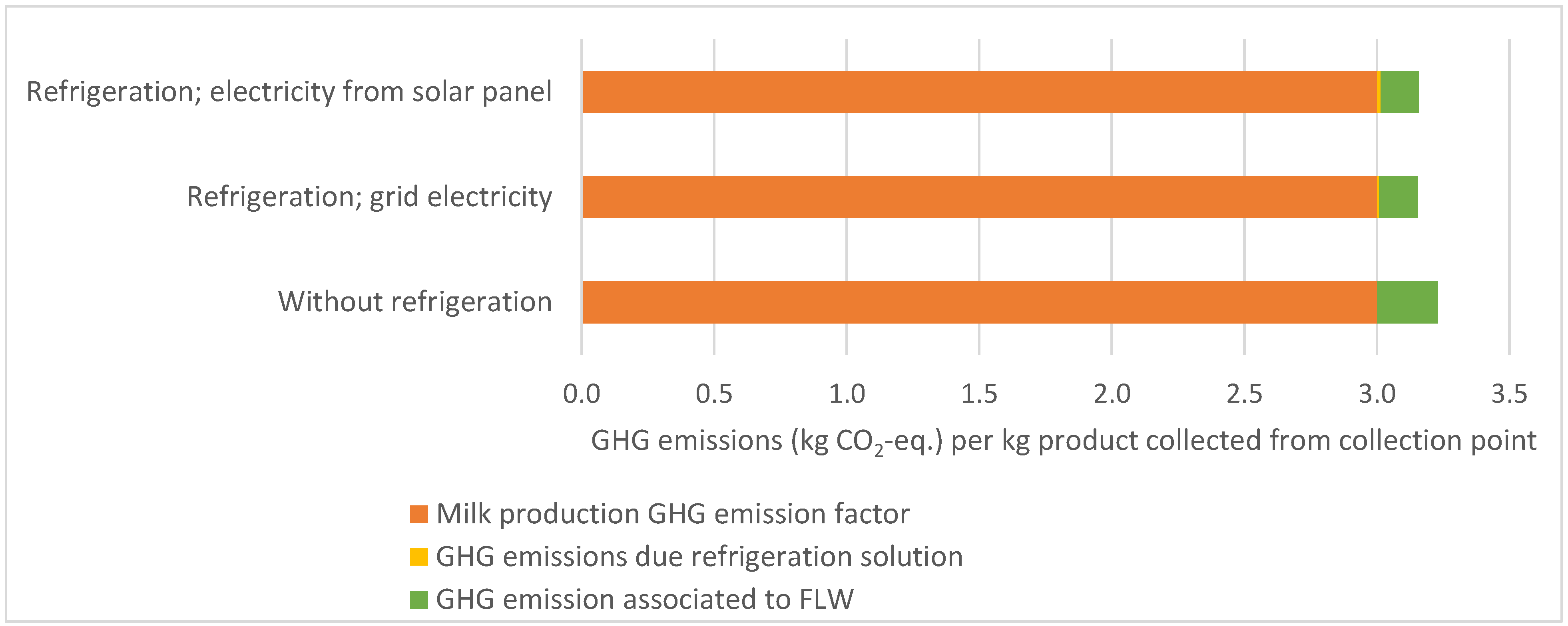
Figure 2. Calculated GHG emissions along the dairy value chain up to collection from the collection point.
Sustainability 15 08531 g002
Figure 3. Total GHG associated with 1 kg bovine meat bought by a consumer for two cooling scenarios.
Sustainability 15 08531 g003
Figure 4. Total GHG associated with 1 kg pre-processed vegetables bought by a consumer for two cold chain scenarios.
Sustainability 15 08531 g004
Figure 5. GHG emissions induced by different operations along the supply chain for melons from Honduras to UK.
Sustainability 15 08531 g005
Table 2. Impact factors and FLW factors for both scenarios.
FactorsValueSource/Comment
Bovine meat GHG emission factor22.9 kg CO2-eq./kg product[1]
Processing/packaging loss factor5%[1]
Retail shelf loss factorCooling at 7 °C: 3%
Cooling at 4 °C: 1%
Estimated with the method presented by [46] for a representative supply chain in the Netherlands
Table 3. Chain configuration parameters for the bovine meat product.
Chain Configuration
Parameters
ValueSource/Comment
Processing energy use-GHG emissions up to meat processing are included in the product’s GHG emission factor and, thus, should not be added to the calculations.
Refrigerated storage duration in processing/packaging stage1.3 dayspractical expert estimate
Packaging plastics0.03 kg plastics per kg meatmeasured from practical samples (random samples from a supermarket)
Transport from the packaging station to the distribution center80 km, large truckpractical expert estimate
Refrigerated storage duration in the distribution center0.5 dayspractical expert estimate
Transport from distribution center to retail shop50 km, large truckpractical expert estimate
average Refrigerated retail display durationCooling at 7 °C: 40 h
Cooling at 4 °C: 45 h
Estimated with the method presented by [46] for representative supply chain in The Netherlands
Table 4. Impact factors and FLW factors for the vegetable product scenarios.
FactorsValueSource/Comment
Vegetable production GHG emission factor0.84 kg CO2-eq./kg product[1]
Handling and storage loss factor7.3%[1]
Processing/packaging loss factor2.0%[1]
Retail shelf loss factorCooling at 7 °C: 3%
Cooling at 4 °C: 1%
Estimated with the method presented by [46] for a representative supply chain in the Netherlands
Packaging plastics0.01 kg plastics per kg productPractical samples measurement
Table 5. Chain and GHG emission parameters for melon supply from Honduras to UK (data provided by Stepac unless otherwise stated).
ParameterValue and Further Specification
Crop GHG emission factor 0.27 kg CO2-eq. per kg crop [50]
Trucking distance from the orchard to the packing house 15 km (non-refrigerated medium size truck)
Operations in the packaging stationCooling down
Cold storage for an average of 2 days
Packaging
Packaging material useCarton: 80 g per kg melon
Plastic (optional): 4 g per kg melon
Intercontinental transport (refrigerated reefer container)Large truck: 386 km
Container ship: 8760 km
Large truck: 20 km
Losses (rejects) at point of arrivalScenario without packaging: 17.5%
Scenario with modified atmosphere packaging: 3.5%
Table 6. Chain and emission parameters for the tomato varieties.
Reference Hybrid
Variety
Variety with Improved Yield (Ayushman)Variety with Improved Shelf Life (Ansal)
Average annual yield (ton/ha)3943.545
Crop GHG emission factor (kg CO2-eq. per kg crop)0.0320.0290.028
Farmer grading: rejects20%3–5%3–5%
Buyer grading: rejects1%1%1%
Loss during long-distance transportation and on market20–25%34–39%8–10%
Transportation from field to collection center20 km; small truck20 km; small truck20 km; small truck
Transportation from collection center to market500 km; medium size truck500 km; medium size truck500 km; medium size truck
Table 7. Chain scenario parameters and GHG emissions (emissions due to cooling, transport, and losses derived with ACE calculator).
Scenario 1.
Current Supply Chain: From Mekong Delta to Amsterdam (By Air)
Scenario 2. Supply Chain: From
Mekong Delta to Rotterdam (By Sea, Reefer Container)
Scenario 3: Equal to Scenario 2,
Supplemented with Cold Storage Directly after
Picking
Total food losses (measured/estimated)15%44%13%
Crop production GHG intensity *14.3 kg CO2-eq./kg14.3 kg CO2-eq./kg14.3 kg CO2-eq./kg
Emissions due to cooling energy use in the collection chain--≪ 0.1 kg CO2-eq./kg
Emissions due to international transport *11 kg CO2-eq./kg0.6 kg CO2-eq. per kg0.5 kg CO2-eq. per kg
Emissions due to post-harvest losses **1.1 kg CO2-eq./kg9.0 kg CO2-eq./kg0.4 kg CO2-eq./kg
TOTAL emissions per kg product on end market26.5 kg CO2-eq./kg24 kg CO2-eq./kg15 kg CO2-eq./kg
* Per unit produced or transported product. ** Emissions due to extra production and transport needed to compensate for the losses.
Disclaimer/Publisher’s Note: The statements, opinions and data contained in all publications are solely those of the individual author(s) and contributor(s) and not of MDPI and/or the editor(s). MDPI and/or the editor(s) disclaim responsibility for any injury to people or property resulting from any ideas, methods, instructions or products referred to in the content.