Abstract
Many applications of water resources planning and management depend on continuous streamflow predictions. A lack of data sources makes it difficult to predict stream flows in many world regions, including Saudi Arabia. Therefore, using simple, parsimonious models is more attractive in areas where data is scarce since they contain few parameters and require minimal input data. This study investigates the ability of simple, parsimonious water balance model models to simulate monthly time series of stream flows for poorly gauged catchments. The modified Schreiber’s empirical model and SIXPAR monthly water balance model were applied to simulate monthly streamflow in six mountainous watersheds located southwest of Saudi Arabia. The SIXPAR model was calibrated on one single gauged catchment where adequate hydrological data were available. The calibrated parameters were then transferred to the ungauged catchments based on transferring information using a physical similarity approach to regionalization. The results show that the simplified Schreiber’s model was found to consistently underestimates the monthly discharge, especially at low and moderate flow. The monthly water balance model SIXPAR based on the regionalization approach was found more capable of producing the monthly streamflow at the ungauged site under all flow conditions. This study’s finding agrees with other studies conducted in the same area using different modeling approaches.
1. Introduction
The streamflow information generated from river basins at specific time scales is needed for several hydrological applications and basic studies concerning water supply, irrigation, hydropower generation, and integrated watershed management.
Understanding the rainfall-runoff behavior of ungauged catchments provides a basis for sustainable water resource management and the understanding of systems behavior.
Water resource management and flood prediction in many countries are compromised by poorly gauged or completely ungauged catchments. Therefore, accurate streamflow modeling and forecasting is a key issue in hydrology for water resources assessment and flood Management [1,2,3,4].
Modeling rainfall-runoff in ungauged catchments is still challenging Due to the lack of local runoff data [5] and the considerable uncertainties associated with modeling [6]. It is important to calibrate model parameters since most model equations are empirical in nature, model output depends on poorly known initial and boundary conditions, and, most importantly, since most flow processes occur under the surface, where media characteristics are heterogeneous and unknown. The properties of soil vary dramatically in space but very little in time, so parameter calibration can greatly enhance model performance.
All over the world, Streamflow forecasting in ungauged basins is seen as a significant challenge. Therefore, a lot of work has been put into solving this problem. However, there is no single best way to do something, and different methods may be more effective in different situations.
Streamflow predictions in ungauged catchments continue to be an active area of research. In many developing countries, many catchments are either inadequately gauged or completely ungauged, making it difficult for these countries to manage their water resources and predict floods. Numerous researchers have used different watershed models to tackle the problem of hydrologic analysis in ungauged watersheds, and Kim and Kaluarachchi [7] have provided a history of parameter estimates for ungauged watersheds.
Most continuous-time rainfall-runoff models come under the conceptual model category [8]. More focus has been placed on the use of conceptual models generally, which primarily benefits from black-box modeling and a calibration process to obtain hydrological parameters and streamflow [9,10] and to simulate groundwater levels [11,12]. The rainfall-runoff process at the catchment scale can be reliably predicted using distributed and conceptual models. However, they do not apply to basins without specific data or parameters [13].
Early attempts to estimate streamflow from ungauged catchments used model parameters that had been calibrated using data from nearby gauged catchments. However, when basin parameters such as geography, land use, and soil type differ significantly from those of gauged catchments, the estimated streamflow from ungauged catchments may contain errors [14,15]. If runoff data are unavailable, we cannot calibrate or validate the watershed model; therefore, we need to use regional methods that can easily relate watershed model parameters to measured watershed characteristics.
Broadly, regionalization methods can be classified based on temporal dimension into two main groups; the first group provides an estimate of streamflow series (e.g., [16,17]). The second group, as an alternative to the estimation of the continuous streamflow series, provides an estimation of some specific hydrological indices (e.g., [18]), or A flow’s various percentiles (e.g., regionalization of the so-called flow duration curve—F.D.C.) [19].
The use of hydrologically similar catchments is a good example of how to estimate model parameters in ungauged catchments. Hydrological similarity assumes that runoff responses to a given rainfall input in two different catchments will be similar if rainfall-runoff processes are similar.
Hydrologic regionalization is the process of transferring model parameter data from gauged to ungauged catchments [20]. In efforts to improve hydrologic models and bring reliable flow prediction in ungauged watersheds as a parallel method to calibration, regional analysis, which transfers certain common information from one catchment to another within a specified homogeneous geographic area, has been utilized extensively [21,22]. Similar characteristics can show similar hydrological behavior; therefore, similar parameters can be used while modeling these catchments [23]. It is assumed that catchment attributes are surrogates of the hydrological processes within a catchment, such as the catchment size, topography, land use, geology, elevation, and soil characteristics.
Some researchers found that transposing a complete set of model parameters performed better than regression [24,25].
Numerous hydrologic regionalization techniques have emphasized creating comparisons of gauged and ungauged catchments based on physical characteristics and spatial proximity. Physical characteristics of the catchment have been employed as exploratory variables to understand better the relationship between model parameters, which indicate model function, and physical properties of the watershed [17].
In efforts to improve hydrologic models and bring reliable flow prediction in ungauged watersheds as a parallel method to calibration, regional analysis, which transfers certain common information from one catchment to another within a specified homogeneous geographic area, has been utilized extensively [21,26], and Important progress is being made to regionalize continuous simulation using parsimonious rainfall-runoff models [25,27]. However, since lack of data continues to be the major issue in many developing nations, simple conceptual water balance models such as ABCD using satellite products as data sources for meteorological variables are suitable tools for simulation [28].
In the present study, an attempt has been was made to compare the modified Schreiber model (Miranda et al., 2002) [29] and the SIXPAR monthly conceptual water balance model proposed by Jazim in 2006 [30] in predicting the monthly water yield of Al Sarwat mountainous watersheds southwest of Saudi Arabia. The main objective is to investigate these simple parsimonious models’ ability to estimate monthly streamflow series satisfactorily using minimum available hydrological data.
2. Materials and Methods
2.1. Study Area and Data
The study area covers 7 watersheds located southwestern part of Saudi Arabia, with areas ranging from 1090 to 4885 km2 adjacent to the southwest coastal region.
Figure 1 shows the location of 7 catchments within the Saudi Arabia map. The largest is the Hali catchment, with an area of 4885 km2, whereas the smallest is the Demad catchment, with only 1090 km2. These catchments cover a large area but have nearly considerable similarities in climatic and physiographic characteristics. For example, the annual precipitation, aridity index, percentage of the forest, and slope vary from 149 to 284 mm, 0.067 to 0.101, 16.8 to 43.2%, and 25.22 to 37.5%, respectively. Watershed characteristics such as size, the x and y coordinates of the centroid, mean annual rainfall, minimum elevation, mean elevation, maximum elevation, and length of rivers are all provided in Table 1.
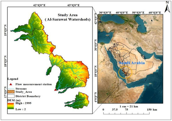
Figure 1.
Location of the study area.

Table 1.
Characteristics of watersheds in the study area.
These watersheds are part of Al Sarawat mountain range that extends from southern Yemen to the beginning of the Gulf of Aqaba. The Kingdom’s share is approximately 1550 km, with a width ranging from 150 km to 40 km. Few studies have been undertaken to assess the potential of water resources in Al Sarawat mountain range. Some reports give some exaggerated figures about the runoff potential of this mountain range, but these figures are not supported by scientific studies and research. This study attempts to assess the potential of water resources in these mountainous watersheds and assess possible utilization through water harvesting.
The ‘SIXPAR’ conceptual model requires a monthly precipitation time series, potential evapotranspiration, and streamflow to conduct calibration and validation. These data are very scarce in these mountainous watersheds. Therefore, the author has collected these data from different sources. The average monthly time series of Streamflow and precipitation for the Baysh watershed was extracted from some published studies and reports conducted on the area; the data were available for 14 years between the years 1977 and 1991 [31,32].
The mean time series of area average of monthly air temperature and time series of area -average of merged satellite-gauge precipitation estimate –Final Run (recommended by NASA for general use) was downloaded from Giovanni website, a Web application developed by the NASA GES/DISC (https://giovanni.gsfc.nasa. gov/giovanni/ (accessed on 12 July 2022)).
GPM-IMERGE product shows good correlation performance in Iran. Furthermore, it is superior to the other products when applied in areas with diverse topography and variable precipitation. In conclusion, the product is suitable for future meteorological and hydrological models application [33]. Furthermore, in Saudi Arabia, IMERG products showed a high correlation between gauge measurements and corresponding satellite estimates in most Saudi Arabia regions [34].
Generally, the GPM-IMERGE product with monthly time step performed well compared to the rain gauge record and could detect monthly rainfall temporally and spatially [35,36,37,38,39,40]. In addition, several other researchers have reported that the IMERG Final-Run product is a reliable source of rainfall data for various hydrological and hydroclimatic studies [41,42,43].
The spatial average of 8-day Potential Evapotranspiration, available through MOD16A2 Version 6 global product, was downloaded from NASA AppEEARS Data Site at (https://appeears.earthdatacloud.nasa.gov/ (accessed on 14 July 2022) ). The MOD16A2 is the sum of 8-day P.E.T. at 500 m spatial resolution [44], providing an estimate for P.E.T. according to toPenman–Monteith equation. Monthly average P.E.T. was calculated from the sum of 8-day P.E.T. This product has been validated across an arid environment with a poor data monitoring system and found beneficial for hydrological application [45].
The digital elevation model, DEM. of the study area, was downloaded from the Nasa website; the DEM is freely available at 30 m resolution. Several DEMs have been downloaded, merged, and composed inside the program to make a single DEM covering the study area and then projected into WGS_1984_UTM_Zone_38N.
DEM was manipulated using ArcGIS 10.4.1 Arc Hydro tools (a version that works with ArcGIS 10.4.1) are used to define the streams and drainage network in the study area and to delineate the watershed boundaries on the bases of DEM. Many data sets that together describe the catchment drainage patterns are derived using the Arc Hydro tools. Data on flow direction, flow accumulation, stream definition, stream segmentation, and watershed delineation are generated using raster analysis. These data are then used to create a vector representation of the watershed and drainage lines from selected points. The result of this process is shown in Figure 1, which illustrates the watershed area of southwestern parts of the Al Sarawat mountain range.
Most of Saudi Arabia’s soil is primarily characterized as shallow to deep soil over bedrock [46]. However, some studies have investigated the properties of Saudi Arabia’s agricultural regions’ soils and reported that the predominant soil textures in these regions are sand, loamy sand, and sandy loam [47].
Since soil studies are very limited in the study area, the Harmonized Global Soil Database (FAO/IIASA/ISRIC/ISSCAS/JRC, 2012) provided the required information on soil data [48]. Therefore, HWSD-Viewer is used to visualize the study area’s dominant soil type and texture. The soil in the study area consists of three major groups: Leptosol, Fluvisols, and Calcisols. The most dominant soil group in the study area is Letosol, with approximately 70%. Table 2 shows the USDA soil texture class and depth for different soil groups in the study area.
Table 2.
USDA soil texture class and depth for different soil groups in the study area.
The main source for the values used for the soil hydraulic conductivity parameter and other soil parameters was taken from Saxton and Rawls (2006) [49].
Landsat 8 O.L.I. & TIRS multispectral band with 30 m spatial resolution were obtained from United State Geological Survey (USGS) (https://earthexplorer.usgs.gov/ (accessed on 8 January 2021)). Google Earth is employed as a high-resolution satellite image to reclassify and identify the changing features in the study area. Erdas Imagine software, version 15, 2015 defines the study area’s land use and land cover features. Satellite image processing based on supervised and unsupervised classification algorithms. Google Earth is used as a high-resolution satellite image to reclassify and identify the changing features. ERDAS Imagine software version 15, 2015 has been used for Pre-processing and Geometric correction of the satellite imagery. Six different classes have been defined for the study area: Agriculture, Baren Land, Rock Outcrop, Urban, Sparse Vegetation, and Dense Vegetation, as illustrated in Figure 2.
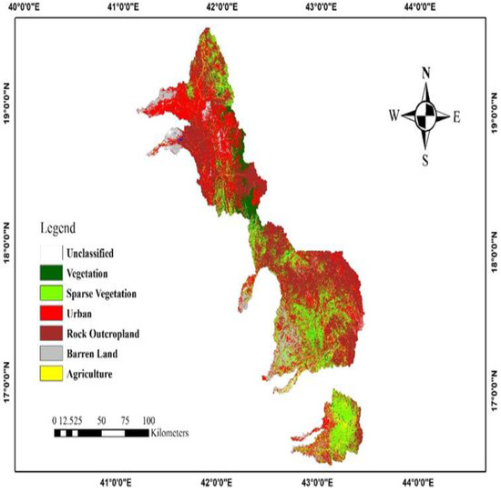
Figure 2.
Land cover classification of the study watersheds produced using ERDAS IMAGINE software, version 15, 2015.
2.2. Modified Schreiber’s Empirical Model
An attempt was made in this study to examine the ability of the modified Schreiber model to provide a satisfactory estimate of catchment yield in a changing climate using only limited available data and commonly available local parameters.
The model showed a good runoff prediction in tropical and sub-tropical areas [50]. The main input parameters for the model are monthly precipitation, monthly atmospheric temperature, and watershed area.
where,
Vq = monthly Runoff Volume (m3/s)
Ax = watershed Area (K2)
e0 = monthly evapotranspiration (mm)
r = monthly rainfall (mm)
Di = number of days in the month
T = monthly Mean Temperature (co)
2.3. SIXPAR Monthly Water Balance Model
Rainfall–runoff model (SIXPAR), developed by Jazim (2006), is a conceptual rainfall–runoff model with six parameters and works with a monthly time steps. This model was developed to suit the condition of arid and semiarid catchments.
The soil moisture storage of the drainage basin is divided into two stores: the upper layer soil moisture store (U.S.M.) and the lower layer soil moisture store (L.S.M.). The model is primarily based on the water balance concept. Each layer in the Jazim model has a unique potential for absorbing and retaining moisture. The lower layer is an intermediate layer over a saturated aquifer, while the upper layer simulates fast runoff and soil moisture storage. Monthly rainfall, pan evaporation, and streamflow records are major input data for the model., and accordingly simulate monthly surface flow, subsurface flow, groundwater flow, and upper and lower soil contents. The SIXPAR model performance in the arid and semiarid regions has been investigated by several researchers [51,52,53,54], and they reported that the model provides a satisfactory simulation of the monthly streamflow time series. Figure 3. shows a schematic representation of the SIXPAR conceptual rainfall–runoff model.
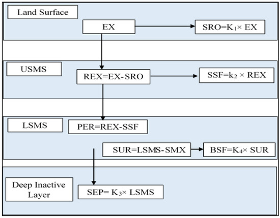
Figure 3.
Schematic of the SIXPAR conceptual rainfall–runoff model.
where,
USMS = upper layer soil moisture content
LSMS = lower layer soil moisture content
USMX = upper layer soil moisture storage capacity (USMX is the first model parameter)
LSMX = lower layer soil moisture storage capacity (LSMX is the second model parameter)
EX = USMS-USMX, excess water above the upper layer soil moisture storage capacity
SRO = K1 × EX surface runoff (K1 is the third model parameter)
R.E.X. = EX-SRO, the remaining excess will flow in part as subsurface flow and in part will percolate downward to augment the lower layer soil moisture storage
SSF = K2 × REX, subsurface flow (K2 is the fourth model parameter)
PER = R.E.X.–S.S.F., percolation to LSMS
SEP = K3 × LSMS, deep seepage (K3 is the fifth model parameter)
S.U.R. = LSMS–LSMX surplus water in excess of the lower layer soil moisture storage capacity
BSF = K4 × SUR, base flow (K4 is the sixth model parameter)
2.4. Hydrological Model Calibration and Evaluation Methods
Obtaining an optimal parameter set that either minimizes or maximizes an objective function of observed and simulated flow is the traditional method for fitting a rainfall-runoff model to the data. Rainfall-runoff modeling has been used to develop and apply numerous objective functions. The proposed model’s performance is evaluated using a variety of objective functions in this study. Each objective function can be used independently or collectively to assess the proposed model’s parameters. The first objective function utilized in this work is the well-known least square objective function, perhaps one of the most frequently used in model calibration. The least squares objective function can be obtained by
when N represents the overall number of months, Qobsi represents the observed flow for a month i, Qsimi represents the simulated flow for month i, and the least square objective function calculates the sum of flow residual. To accurately simulate the monthly runoff, the value of OF must be close to zero.
Nash efficiency criterion, defined as in Equation (4), is used as an additional optimization method.
where is the observed streamflow during the calibration period N. A value of R2 close to 100 percent indicates a perfect agreement between the observed and simulated flows. In contrast, a negative R2 indicates a lack of agreement worse than if the simulated flows were replaced with the observed monthly flow.
The degree of agreement between the simulated and observed hydrographs is shown by the coefficient of determination R2. The coefficient of determination, R2, is expressed in Equation (5) below,
an additional criterion, the relative error in volume, RE, between the observed and simulated flow, has been used to assess the model prediction accuracy. The relative error in volume, RE is defined by
RE should be close to zero to ensure a good match between the observed and simulated total volume.
The optimization method known as Shuffled Complex Evolution (SCE.UA), developed by Duan et al., (1992), is utilized in this study to optimize the SIXPAR model’s parameters. A powerful global optimization method, SCE.UA, was initially developed to address the peculiarities encountered during conceptual watershed model calibration.
2.5. Regionalization Methods
Regression-based and donor-based methods are the two basic categories into which the regionalization techniques may be divided. A physical similarity or donor-based regionalization method has been employed in this study. Donor-based methods attempt to locate a suitable donor-gauged watershed (or watersheds) most similar to the target ungauged watershed and transfer the complete set of donor parameters from this watershed to the ungauged watershed. Then, suitable donor watersheds are chosen based on the hydrologic similarities between the gauged and ungauged watersheds. In many regions, the physical similarity method is more effective [55,56,57].
Methods for comparing physical similarity are based on watershed characteristics, including mean elevation, types of forest cover, and soil types [24,58,59].
These techniques are founded on the notion that hydrological behavior might be comparable amongst geographically separated catchments. With the physical similarity method, donor catchments are chosen based on their characteristics on the basis that catchments with comparable characteristics may behave similarly in hydrological processes [60,61].
The similarity index suggested by Burn & Boorman [62], which is generated using the following formula, was employed in this study:
where CD stands for “catchment descriptor,” “d” for “donor catchment,” “t” for “target catchment,” “k” stands for “total number of catchment descriptors,” and “CDi” stands for “range of ith catchment descriptor.”
In this study, the Baysh watershed has been selected as a donor watershed, where six catchment descriptors have been selected, as listed in Table 3. The catchment descriptors include; slope, percentage of the forest, mean annual precipitation, mean annual evapotranspiration, drainage density (DD), and aridity index. All catchment descriptors were used to investigate the similarity between Baysh and other ungauged watersheds in the study area.
Table 3.
List of catchment descriptors used in the regionalization.
3. Results and Discussion
3.1. Calibration and Validation of the SIXPAR Model
Wadi Baysh catchment was selected as a donor catchment, where the SIXPAR model has been calibrated and validated using the available limited data. Available observed stream flows were used for calibration and validation for 1977–1983 and 1984–1991. The performance of the SIXPAR model shows a good agreement between the monthly time series of streamflow during the calibration and validation period. The simulation results are shown in Figure 4, along with the values of a performance criterion, such Nash- Sutcliff criterion, E, and coefficient of determination, R.
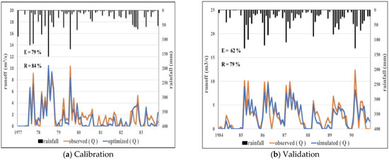
Figure 4.
Wadi Baysh observed and simulated monthly runoff hydrograph. (a) calibration period (1977–1983) and (b) validation period (19984–1991).
The coefficient of efficiency, E, is 79% for calibration and 62% for validation. The coefficient of determination, R, ranges from 84% during calibration to 79% during validation.
The relative error in volume and RE between the observed and simulated streamflow was less than 10% during calibration and validation. The total simulated flow volume is within 9% of the total recorded flow volume during the optimization and within 6% of the total recorded flow volume during the validation. It’s evident that during the calibration, the values of RE are always higher than the validation. The SIXPAR performance was satisfactory on Wadi Baysh, with better performance obtained during the calibration period. The optimized parameter values for the SIXPAR model were obtained for the Wadi Byash catchment and presented in Table 4.
Table 4.
SIXPAR optimum parameters with their lower and upper bound.
The SIXPAR performance was satisfactory on Wadi Baysh, with better performance obtained during the calibration period. As a result, the optimum parameter values for the SIXPAR model were obtained for the Wadi Byash catchment and presented in Table 5. Most of the parameters take values closer to their lower bound except Lower Soil Moisture Storage, LSMS which takes value closer to its upper bound; this is because, unlike upper soil, which is continuously depleted through evapotranspiration and seepage, the lower soil layer contains more clay and silt ratio and therefore has higher water moisture holding capacity and tend to retain water for a longer time. As a result, the majority of monthly streamflow is made up of direct surface runoff; this is due to the nature of the watershed in the study area, where the majority of surface runoff occurs in mountainous parts of the watershed where rain typically falls at high intensity. In addition, other driving factors, like steep slopes, shallow water, and rock outcrops, make the conditions more favorable for surface runoff. Normal precipitation can be intercepted and held in the plant’s canopy, fall to the soil’s surface, or evaporate away later. The heavy rain causes water to flow overland as runoff, accelerate toward a stream channel, and contribute to the short-term response of the stream. Water begins infiltrating the subsurface at the lower reach of Wadi courses, particularly where superficial deposits or porous sedimentary rocks are present.
Table 5.
Sensitivity analysis of the proposed model parameters (when parameters values increase by 10%).
Base flow at a substantial rate in the study area; this is evident from the high value of parameter k4. During winter floods, groundwater recharge occurs exclusively. If the amount of water in that layer exceeds the field capacity for water, water can percolate from the upper soil layer into the lower layer. Percolated water enters and flows into the shallow aquifer through the vadose zone, where it reaches the lowest depth of the soil profile. Deep seepage is a fraction of percolated water and occurs continuously from lower soil storage, but as noted in Table 4, the value of K3 is small, indicating that deep seepage occurs at a lower rate than the rate of base flow. Base flow depends on the available moisture content in the lower soil layers. When the moisture content of the lower soil layer exceeds the maximum holding capacity, the base flow originates. In this study, the physical similarity method of regionalization has been adopted based on the resemblance of hydrological behavior between the donor-gauged catchment and other ungauged catchments in the study area. The parameters set calibrated in Wadi Baysh have been transferred to six other ungauged catchments for streamflow prediction. Figure 5 illustrates the results of streamflow prediction using the SIXPAR model at the selected ungauged watersheds in the study area based on 20 years of historical data.
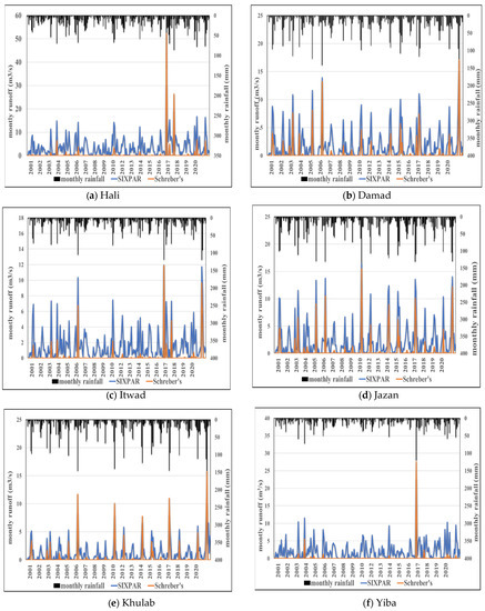
Figure 5.
Time series of monthly runoff in ungauged watersheds simulated by the SIXPAR conceptual model and Schreiber’s empirical model (from 2001–2020).
In the same figure, the results of streamflow prediction using the modified Schreiber’s empirical model are also provided. The results reveal that the SIXPAR conceptual water balance model performs well in runoff prediction under all stream conditions. However, Schreiber’s empirical model overestimated high streamflow in the dry watershed while underestimating low streamflow in the wet watershed; this may happen due to the nature Schreiber function, which relates the ratio of actual evapotranspiration to precipitation. When the monthly precipitation (P) exceeds the monthly amount of potential evapotranspiration (P.E.), the remaining precipitation will soak into the ground to replenish soil moisture and run off as streamflow. The large number of outliers in Figure 5 makes the Schreiber empirical model less useful in watersheds with primarily arid or semiarid climates, making it an unsatisfactory method for estimating monthly runoff.
3.2. Uncertainty Analysis
3.2.1. Sensitivity Analysis of the SIXPAR Model Parameters
As a crucial step in model uncertainty analysis, sensitivity analysis was carried out to investigate the sensitivity of the SIXPAR model to the variation of parameter values. Operational projects for managing water resources should always take into account and evaluate uncertainty in streamflow estimation [63].
While each parameter was altered within a ten percent range of the optimal value, the remaining model parameters’ optimal values were maintained. The results of the sensitivity analysis are shown in Table 5 and Table 6. The SIXPAR model was extremely sensitive to USMX (moisture in the upper soil layer); the SEN values for an increase and decrease in the value of USMX are 28.29 and 42.74, respectively, which is a very high value. This high sensitivity was because USMX mainly controls the runoff generation process, and therefore this parameter is expected to have high sensitivity in surface runoff simulation. Also, since USMX takes a value closer to its lower constraint, the available soil moisture storage capacity is very limited, and the moisture level at the catchments soil is always greater than the field capacity; therefore, the excess water above the upper layer of soil moisture storage capacity augment surface runoff continuously.
Table 6.
Sensitivity analysis of the proposed model parameters (when parameters values decrease by 10%).
The sensitivity measures for LSMX range from 12.81 to 29.56 for a 10% increase and decrease in the parameter value, which is a significant value. LSMX is augmented by percolation from the upper layer soil store and causes keep moisture in this layer within its field capacity because this parameter takes value closer to its lower constrain, and hence small change in the parameter value is expected to have a great impact on base flow and deep percolation and consequently on the objective function.
The SEN value for surface runoff coefficient, k1, varies between 9.63 and 17.56 for a 10% increase and decrease in the parameter value, which indicates that K1 is also a sensitive parameter since this parameter has a direct relation with the process of runoff generation, and has strong interactions with other parameters such as LMSX, interflow coefficient, K2 and deep seepage coefficient k3. Therefore, a small variation of this parameter is expected to greatly impact other runoff components, such as subsurface and base flow.
Interflow coefficient k2 is taking value near to its lower constraint. This parameter has nearly the same SEN value for a 10% increase and decreases around its optimum value. The SEN value is insignificant, indicating that k2 is an insensitive parameter. Interflow is common in mountain soils, where vegetation can form a layer with high porosity on the surface. However, the situation is reversed in relatively bare soil, as in most arid and semiarid catchments. Interflow co-efficient K2 should always be optimized under all modeling conditions Since it is very difficult to predict its occurrence and relate it to watershed characteristics.
Baseflow coefficient, K3 has a SEN value range from 3.037 to 6.89 when changing its value by more than or less than 10% about the optimal value, which indicates that K3 has small to medium, medium sensitivity. The baseflow component is fundamental to stream runoff in arid and semiarid watersheds. The thermal regime, geological conditions, land cover, precipitation, temperature, and soil moisture can impact it. In the SIXPAR model, the primary source for baseflow is the recharge from precipitation, which continuously replenishes the soil layer’s moisture and keeps it near its field capacity level. In the study area, as the air temperature rises, evapotranspiration can increase while precipitation infiltration and soil water decrease further; therefore, the baseflow component contributes little to the total streamflow compared to surface and subsurface runoff.
The coefficient of deep seepage, k4 has the lowest SEN value; the value is closer to zero. Deep seepage is associated with the available moisture in the lower soil layer, which is always depleted by evapotranspiration and baseflow. In this study, the lower value for LSMX induces the occurrence of baseflow and reduces the deep seepage. Soils in high mountain watersheds of the study area are characterized by a thin surface layer and shallow depth and have a very low deep percolation rate; therefore, K3 is the less sensitive parameter since the deep seepage component is not significant in the study area and has little influence on the process of streamflow generation. Nevertheless, the above analysis reveals that the USMX, LSMX, and K1 are the most sensitive model parameters; therefore, these parameters should be optimized properly under all modeling conditions.
Similar results were obtained when SIXPAR for the simulation of water balance processes in Karaj Basin, central Iran, where it was reported that parameters USMX and K1 demonstrate the highest sensitivity [51]. Another study showed that the SIXPAR model parameter LSMX is the most sensitive and has the greatest significant impact on the uncertainty of runoff [64].
3.2.2. Flow Duration Curve
FDCs can be useful for identifying and characterizing the uncertainty of hydrological models. By comparing the observed and simulated FDCs, it is possible to identify areas of uncertainty and improve the accuracy and reliability of hydrological models.
Figure 6 shows the flow duration curves (FDC) of the observed and simulated streamflow for the Wadi Baysh catchment during the validation period. The SIXPAR model detected the change in the flow regime, but it was not accurate enough for exact reproduction. As a result, the SIXPAR model tends to underestimate streamflow values during the peak period.
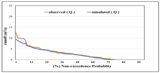
Figure 6.
Flow duration curves (FDC) of monthly streamflow for the Wadi Baysh catchment during the validation period (1984–1991).
The underestimation of high flows can result from several factors, including catchment processes and the input and flow data, and is highly influenced by smaller scales in space and time variations of elevation and precipitation. The rainfall rate during spring and summer seasons with steep slopes in the mountainous area upstream of the studied watersheds are the main cause of flooding. Flash floods originate in the mountainous parts of the watersheds due to high-intensity rainfall occurring within a short duration and is the main cause of the peak flow. Unfortunately lumped conceptual model cannot identify the full range of this process since the lumped modeling approach considers a watershed as a single unit and generally doesn’t consider the spatial distribution of input data, such as the variations of precipitation and watershed characteristics.
Compared to the wet period, the performance of SIXPAR is significantly improved during the dry period. This is because the SIXPAR simulation structure does not consider all the parameters that affect runoff production and variability in the wet period. However, the performance is better in the dry period because there is less uncertainty. Conceptual models are simplified representations of real-world hydrological processes that are used to estimate surface runoff and other hydrological variables. However, these models are often based on assumptions and simplifications that can lead to underestimation of surface runoff.
One common issue with conceptual models is the assumption of uniform rainfall across the catchment area. However, rain can vary significantly across a catchment due to topography, vegetation cover, and land use. Therefore, if the model assumes uniform rainfall, it may underestimate the surface runoff because it does not consider the spatial variability of rainfall.
Another issue is the assumption of constant soil properties throughout the catchment area, such as soil infiltration capacity and hydraulic conductivity. In reality, soil properties can vary significantly within a catchment due to soil type, texture, and structural differences. Therefore, if the model assumes constant soil properties, it may underestimate the surface runoff because it does not account for the spatial variability of soil properties. Additionally, conceptual models may not fully account for the effects of antecedent moisture conditions, which can significantly impact surface runoff. For example, suppose the catchment is saturated or has high soil moisture content due to previous rainfall events. In that case, the surface runoff will be higher than if the catchment was dry before the rainfall event. If the model does not account for these antecedent moisture conditions, it may underestimate the surface runoff. In summary, conceptual models can underestimate surface runoff due to various factors, including assumptions of uniform rainfall, constant soil properties, lack of consideration of antecedent moisture conditions, and failure to account for the effects of human activities.
The underestimation of the peak flow is one of the key issues in hydrological modeling. Still, it poses challenges to modeling with simple spatially lumped conceptual models and more complex physically based hydrological models such as SWAT [29,65,66,67,68].
3.3. Models Performance Comparison
Figure 7 displays the simulation results of both the SIXPAR and Schreiber’s models during the wettest month (August) within the simulation period at the Khulab watershed for [2001–2020]. The figure presents a comparison between observed and simulated runoff values by the SIXPAR and Schreber’s models in the wettest month (August) for the simulation period (2001–2020), allowing for a comparison between the two models. The results indicate that the SIXPAR model produces the best results in estimating the wettest month runoff. However, Schreiber’s model tends to overestimate the wettest month runoff. Similarly, Figure 8 illustrates the simulation results of the SIXPAR and Schreiber’s models at the Khulab watershed in the driest months (Novembre–February) during the simulation period. Schreiber’s model’s worst performance was during the dry months (Novembre–February) since the model failed to generate the monthly runoff when the monthly rainfall depths were less than 30 mm. SIXPAR model outperformed Schreiber’s model during both the wettest and driest periods. However, the modified Schreiber’s model exhibited poor performance when used to simulate water balance in arid and semiarid watersheds. As a result, it is not recommended to use this model for such applications. The modified Schreiber model is a simple method for estimating the water balance of a catchment based on precipitation and evapotranspiration. However, it may not be able to generate low flow in arid watersheds due to several reasons. One reason is that the model assumes that surface runoff and groundwater recharge are generated solely from precipitation. In arid watersheds, the amount of precipitation is often low and irregular, which can result in low surface runoff and groundwater recharge.
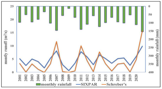
Figure 7.
Comparison between observed and simulated runoff values by the SIXPAR and Schreiber’s models in the wettest month (August) for the simulation period (2001–2020).
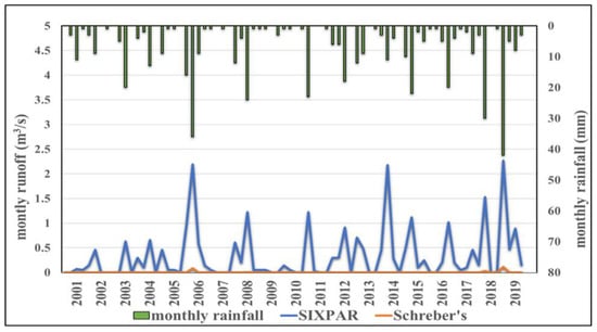
Figure 8.
Comparison between observed and simulated runoff values by the SIXPAR and Schreiber’s models during the driest period of the year (Novembre–February) for the simulation period (2001–2020).
Table 7 compares the performance of the annual water balance prediction between the SIXPAR conceptual model and other models. The comparison results indicate a relative convergence in the prediction ability between the SIXPAR conceptual model and the physically based hydrological model (SWAT) in estimating the annual runoff volume. It was also found that the annual runoff volume estimated by the SIXPAR model is somewhat close to the observed annual runoff values documented in some studies that included some old and limited historical data for the annual runoff volume values in some drainage basins of the study area [69].
Table 7.
Comparison of prediction performance of annual water balance for SIXPAR, Schreiber’s, and Swat models.
Although both SIXPAR and SWAT models provided a good prediction for annual water balance, they have marked differences in their performance when simulating the different components of the total streamflow. Table 8 illustrates the proportion of interflow and baseflow contributions or the percentage of baseflow and interflow components to the total streamflow when SIXPAR and SWAT models were used to simulate water balance in the study area. The results indicate that the interflow and baseflow accounted for 17 to 34% of the annual streamflow in the Al Sarwat watersheds when the simulation was performed using the SIXPAR conceptual model, whereas the percentage contribution of the interflow and base flow range from 11 to 98% when the simulation is performed using SWAT model. Based on SIXPAR simulation results, the dominant streamflow component (Table 8) was the overland flow, followed by interflow from the soil horizon.
Table 8.
Percentage contribution of the interflow and baseflow components to the total streamflow at Al Sarwat mountainous watersheds.
The SIXPAR model produces a more objective estimate for the percentage contribution of the baseflow and interflow since the rivers and streams in the study area are typically characterized as intermittent and ephemeral, which is likely not sustained by baseflow and interflow. Watersheds in dryland environments frequently exhibit lower infiltration capacities and shallow soils with lower soil moisture storage capacities in contrast to watersheds in more humid regions. Therefore, surface runoff is an important flow pathway from these watershed lands. These watersheds generally respond more quickly, with relatively higher peak streamflows for a given amount of rainfall excess than watersheds in other regions. Furthermore, the streamflow is often ephemeral or intermittent because of a lack of soil moisture storage, deep groundwater, and relatively low and frequently sporadic precipitation input. As a result of high temperatures, the annual potential evapotranspiration always exceeds the quantity of annual precipitation. The resulting streamflow tends to be dominated by overland flow (quick flow) that generate flash flood. Due to the high intensity of rainfall and the high percentage of bare soil, rapid flow is very common in arid and semiarid regions.
Consequently, large aquifers do not exist in most locations with a high proportion of rapid flow. Under the climate condition in the study area, the floors of alluvial basins are drying out, and the groundwater beneath them is getting very little recharge. There is very little soil in the upper parts of the catchments to store water. The mountain’s slopes are very steep, and most of the hills cover by impervious rocks. Therefore, retention of moisture by filling the depressions and infiltration is negligible. In the lower portion of the watersheds, because the high-intensity rain quickly seals the bare soil surface, only a shallow depth of soil moisture can be reached before ponding, and surface runoff begins.
The results are in line with similar studies conducted in semiarid watersheds in South Africa and the united states [70,71].
4. Conclusions
This study uses a physical similarity regionalization approach valid for regions characterized by similar physiographic and climatic characteristics. It was successfully applied to one gauged and six ungauged mountainous watersheds southwest of Saudi Arabia. First, the SIXPAR monthly conceptual model was implemented and successfully calibrated and validated at Baysh watersheds (NSE = 79 percent, R = 84 percent during calibration); During validation, NSE = 62 percent, R = 79 percent). After finding the optimal set of parameters of the SIXPAR model at the Baysh watershed, the entire parameters set was transferred to a similar ungauged watershed in the study area.
The SIXPAR conceptual model’s performance was compared with Schreiber’s empirical model in simulating monthly surface runoff in ungauged watersheds. The findings demonstrate that the simplified Schreiber’s model consistently underestimates the monthly discharge time series, particularly at low and moderate flow. On the other hand, the monthly water balance model SIXPAR based on the regionalization approach demonstrates better runoff prediction performance at the ungauged site under all stream conditions.
The methodology employed in this study is applied to a watershed with a low density of rainfall stations and limited streamflow data. This study provides evidence for using a simple, parsimonious conceptual hydrological model as an easy and cost-effective option for predicting water balance in arid and semiarid regions. The results of this study will assist hydrologists in comprehending the effectiveness and application of various rainfall-runoff models, as well as the extent to which parsimonious conceptual and empirical models can be used to estimate streamflow in ungauged watersheds accurately.
Observing the precipitation distribution is necessary to accurately analyze the potential for the development of water resources and create a development plan. The study area currently has several rain gauge stations. Nonetheless, the observation system is poorly managed, resulting in a lack of fundamental data. Also, wadi discharge requires improved monitoring. Consequently, it is essential to establish a monitoring network and intensify efforts to collect and analyze observed streamflow data in ungauged watersheds properly.
This study didn’t account for many anthropogenic issues, such as land use and land cover changes which might have disrupted the hydrological response and functioning of the catchments. The change in vegetation cover and land use cause great alteration to the watershed surface feature, which may have greatly impacted the soil moisture holding capacity and the runoff generation processes. In contrast, the numerous dams constructed over the past few years in the studied watersheds may disrupt the hydrological regime. As a result, improvements must be made in future studies so that these dams can be considered when estimating the long-term water balance. These improvements are essential so that the models can be used to forecast the impacts of global changes in the region to overcome the significant water shortage problem.
The current method’s reliability may be enhanced by applying it to a larger study area with a greater number of watersheds and greater watershed attribute variability.
Author Contributions
The author A.A.J.G. has the sole responsibility for the study conception and design, data curation, analysis and interpretation of results, and manuscript preparation. All authors have read and agreed to the published version of the manuscript.
Funding
This research was funded by the Deanship of Scientific Research at Najran University–Kingdom of Saudi Arabia under code number (NU/NRP/SERC/12/3).
Institutional Review Board Statement
Not applicable.
Informed Consent Statement
Not applicable.
Data Availability Statement
The data is available in the manuscript.
Acknowledgments
The author thanks the Deanship of Scientific Research at Najran University for funding this work under the Research Priorities program (NU/NRP/SERC/12/3).
Conflicts of Interest
The author declares no conflict of interest.
References
- Kamruzzaman, M.; Shahriar, M.S.; Beecham, S. Assessment of Short Term Rainfall and Stream Flows in South Australia. Water 2014, 6, 3528–3544. [Google Scholar] [CrossRef]
- Zhao, N.; Yu, F.; Li, C.; Wang, H.; Liu, J.; Mu, W. Investigation of Rainfall-Runoff Processes and Soil Moisture Dynamics in Grassland Plots under Simulated Rainfall Conditions. Water 2014, 6, 2671–2689. [Google Scholar] [CrossRef]
- Wu, M.C.; Lin, G.F. An Hourly Streamflow Forecasting Model Coupled with an Enforced Learning Strategy. Water 2015, 7, 5876–5895. [Google Scholar] [CrossRef]
- Liu, Y.; Sang, Y.F.; Li, X.; Hu, J.; Liang, K. Long-Term Streamflow Forecasting Based on Relevance Vector Machine Model. Water 2016, 9, 9. [Google Scholar] [CrossRef]
- Pilgrim, D.H.; Chapman, T.G.; Doran, D.G. Problèmes de La Mise Au Point de Modèles Pluie-Écoulement Dans Les Régions Arides et Semi-Arides. Hydrol. Sci. J. 1988, 33, 379–400. [Google Scholar] [CrossRef]
- Sivapalan, M.; Takeuchi, K.; Franks, S.W.; Gupta, V.K.; Karambiri, H.; Lakshmi, V.; Liang, X.; McDonnell, J.J.; Mendiondo, E.M.; O’Connell, P.E.; et al. IAHS Decade on Predictions in Ungauged Basins (PUB), 2003–2012: Shaping an Exciting Future for the Hydrological Sciences. Hydrol. Sci. J. 2003, 48, 857–880. [Google Scholar] [CrossRef]
- Kim, U.; Kaluarachchi, J.J. Application of Parameter Estimation and Regionalization Methodologies to Ungauged Basins of the Upper Blue Nile River Basin, Ethiopia. J. Hydrol. 2008, 362, 39–56. [Google Scholar] [CrossRef]
- Wheater, H.S. Progress in and Prospects for Fluvial Flood Modelling. Philos. Trans. R. Soc. Math. Phys. Eng. Sci. 2002, 360, 1409–1431. [Google Scholar] [CrossRef]
- Ghanim, A.A.J. Modeling Rainfall Runoff Relations at Arid Catchments Using Conceptual Hydrological Modeling Approach. Indian J. Sci. Technol. 2020, 13, 329–339. [Google Scholar] [CrossRef]
- Ghanim, A.A.J.; Beddu, S.; Sabariah, T.; Abd, B.; Al Yami, S.H.; Irfan, M.; Nasar, S.; Mursal, F.; Liyana, N.; Kamal, M.; et al. Prediction of Runoff in Watersheds Located within Data-Scarce Regions. Sustainability 2022, 14, 7986. [Google Scholar] [CrossRef]
- Aqili, S.W.; Hong, N.; Hama, T.; Suenaga, Y.; Kawagoshi, Y. Application of Modified Tank Model to Simulate Groundwater Level Fluctuations in Kabul Basin, Afghanistan. J. Water Environ. Technol. 2016, 14, 57–66. [Google Scholar] [CrossRef]
- Hong, N.; Hama, T.; Suenaga, Y.; Aqili, S.W.; Huang, X.; Wei, Q.; Kawagoshi, Y. Application of a Modified Conceptual Rainfall-Runoff Model to Simulation of Groundwater Level in an Undefined Watershed. Sci. Total Environ. 2016, 541, 383–390. [Google Scholar] [CrossRef]
- Lin, Y.; Wen, H.; Liu, S. Surface Runoff Response to Climate Change Based on Artificial Neural Network (ANN) Models: A Case Study with Zagunao Catchment in Upper Minjiang River, Southwest China. J. Water Clim. Chang. 2019, 10, 158–166. [Google Scholar] [CrossRef]
- Jeon, J.H.; Lim, K.J.; Engel, B.A. Regional Calibration of SCS-CN L-THIA Model: Application for Ungauged Basins. Water 2014, 6, 1339–1359. [Google Scholar] [CrossRef]
- Vis, M.; Knight, R.; Pool, S.; Wolfe, W.; Seibert, J. Model Calibration Criteria for Estimating Ecological Flow Characteristics. Water 2015, 7, 2358–2381. [Google Scholar] [CrossRef]
- Magette, W.L.; Shanholtz, V.O.; Carr, J.C. Estimating Selected Parameters for the Kentucky Watershed Model from Watershed Characteristics. Water Resour. Res. 1976, 12, 472–476. [Google Scholar] [CrossRef]
- Merz, R.; Blöschl, G. Regionalisation of Catchment Model Parameters. J. Hydrol. 2004, 287, 95–123. [Google Scholar] [CrossRef]
- Nathan, R.J.; McMahon, T.A. Evaluation of Automated Techniques for Base Flow and Recession Analyses. Water Resour. Res. 1990, 26, 1465–1473. [Google Scholar] [CrossRef]
- Castellarin, A.; Vogel, R.M.; Brath, A. A Stochastic Index Flow Model of Flow Duration Curves. Water Resour. Res. 2004, 40, 3104. [Google Scholar] [CrossRef]
- Blöschl, G.; Sivapalan, M. Scale Issues in Hydrological Modelling: A Review. Hydrol. Process. 1995, 9, 251–290. [Google Scholar] [CrossRef]
- Vandewiele, G.L.; Xu, C.Y.; Huybrechts, W. Regionalisation of Physically-Based Water Balance Models in Belgium. Application to Ungauged Catchments. Water Resour. Manag. 1991, 5, 199–208. [Google Scholar] [CrossRef]
- Wagener, T.; Wheater, H.S. Parameter Estimation and Regionalization for Continuous Rainfall-Runoff Models Including Uncertainty. J. Hydrol. 2006, 320, 132–154. [Google Scholar] [CrossRef]
- Bárdossy, A. Hydrology and Earth System Sciences Calibration of Hydrological Model Parameters for Ungauged Catchments. Hydrol. Earth Syst. Sci 2007, 11, 703–710. [Google Scholar] [CrossRef]
- Parajka, J.; Merz, R.; Blöschl, G. A Comparison of Regionalisation Methods for Catchment Model Parameters. Hydrol. Earth Syst. Sci. 2005, 9, 157–171. [Google Scholar] [CrossRef]
- Wagener, T.; Wheater, H.S.; Gupta, H.V. Rainfall-Runoff Modelling in Gauged and Ungauged Catchments; Imperial College Press: London, UK, 2004. [Google Scholar] [CrossRef]
- Hundecha, Y. Regionalization of Parameters of a Conceptual Rainfall-Runoff Model. Available online: https://www.researchgate.net/publication/35658824_Regionalization_of_parameters_of_a_conceptual_rainfall-runoff_model (accessed on 16 January 2023).
- Hong, X.; Guo, S.; Chen, G.; Guo, N.; Jiang, C. A Modified Two-Parameter Monthly Water Balance Model for Runoff Simulation to Assess Hydrological Drought. Water 2022, 14, 3715. [Google Scholar] [CrossRef]
- Baseri, M.; Mahjoobi, E.; Rafiei, F.; Baseri, M. Evaluation of ABCD Water Balance Conceptual Model Using Remote Sensing Data in Ungauged Watersheds (a Case Study: Zarandeh, Iran). Environ. Earth Sci. 2023, 82, 126. [Google Scholar] [CrossRef]
- De Miranda, L.B. Princípios de Oceanografia Física de Estuários; Edusp: São Paulo, Brazil, 2002; Volume 42. [Google Scholar]
- Jazim, A.A. A Monthly Six-Parameter Water Balance Model and Its Application at Arid and Semiarid Low Yielding Catchments. J. King Saud Univ. Eng. Sci. 2006, 19, 65–81. [Google Scholar] [CrossRef]
- Al-Turki, S. Water Resources in Saudi Arabia with Particular Reference to Tihama Asir Province. Ph.D. Thesis, Durham University, Durham, UK, 1995. [Google Scholar]
- Japan International Cooperation Agency (JICA). The Study on Master Plan on Renewable Water Resources Development in the Southwest Region in the Kingdom of Saudi Arabia; Japan International Cooperation Agency (JICA): Chiyoda, Japan, 2010; Volume 3. [Google Scholar]
- Sharifi, E.; Steinacker, R.; Saghafian, B. Assessment of GPM-IMERG and Other Precipitation Products against Gauge Data under Different Topographic and Climatic Conditions in Iran: Preliminary Results. Remote Sens. 2016, 8, 135. [Google Scholar] [CrossRef]
- Mahmoud, M.T.; Al-Zahrani, M.A.; Sharif, H.O. Assessment of Global Precipitation Measurement Satellite Products over Saudi Arabia. J. Hydrol. 2018, 559, 1–12. [Google Scholar] [CrossRef]
- Maghsood, F.F.; Hashemi, H.; Hosseini, S.H.; Berndtsson, R. Ground Validation of GPM IMERG Precipitation Products over Iran. Remote Sens. 2019, 12, 48. [Google Scholar] [CrossRef]
- Mahmoud, M.T.; Mohammed, S.A.; Hamouda, M.A.; Mohamed, M.M. Impact of Topography and Rainfall Intensity on the Accuracy of IMERG Precipitation Estimates in an Arid Region. Remote Sens. 2020, 13, 13. [Google Scholar] [CrossRef]
- Nascimento, J.G.; Althoff, D.; Bazame, H.C.; Neale, C.M.U.; Duarte, S.N.; Ruhoff, A.L.; Gonçalves, I.Z. Evaluating the Latest IMERG Products in a Subtropical Climate: The Case of Paraná State, Brazil. Remote Sens. 2021, 13, 906. [Google Scholar] [CrossRef]
- Nadeem, M.U.; Ghanim, A.A.J.; Anjum, M.N.; Shangguan, D.; Rasool, G.; Irfan, M.; Niazi, U.M.; Hassan, S. Multiscale Ground Validation of Satellite and Reanalysis Precipitation Products over Diverse Climatic and Topographic Conditions. Remote Sens. 2022, 14, 4680. [Google Scholar] [CrossRef]
- Ramadhan, R.; Yusnaini, H.; Marzuki, M.; Muharsyah, R.; Suryanto, W.; Sholihun, S.; Vonnisa, M.; Harmadi, H.; Ningsih, A.P.; Battaglia, A.; et al. Evaluation of GPM IMERG Performance Using Gauge Data over Indonesian Maritime Continent at Different Time Scales. Remote Sens. 2022, 14, 1172. [Google Scholar] [CrossRef]
- Anjum, M.N.; Irfan, M.; Waseem, M.; Leta, M.K.; Niazi, U.M.; Rahman, S.U.; Ghanim, A.; Mukhtar, M.A.; Nadeem, M.U. Assessment of PERSIANN-CCS, PERSIANN-CDR, SM2RAIN-ASCAT, and CHIRPS-2.0 Rainfall Products over a Semi-Arid Subtropical Climatic Region. Water 2022, 14, 147. [Google Scholar] [CrossRef]
- Mahmoud, M.T.; Hamouda, M.A.; Mohamed, M.M. Spatiotemporal Evaluation of the GPM Satellite Precipitation Products over the United Arab Emirates. Atmos. Res. 2019, 219, 200–212. [Google Scholar] [CrossRef]
- Wei, L.; Jiang, S.; Ren, L.; Zhang, L.; Wang, M.; Duan, Z. Preliminary Utility of the Retrospective IMERG Precipitation Product for Large-Scale Drought Monitoring over Mainland China. Remote Sens. 2020, 12, 2993. [Google Scholar] [CrossRef]
- Freitas, E.d.S.; Coelho, V.H.R.; Xuan, Y.; de C.D. Melo, D.; Gadelha, A.N.; Santos, E.A.; Galvão, C.d.O.; Ramos Filho, G.M.; Barbosa, L.R.; Huffman, G.J.; et al. The Performance of the IMERG Satellite-Based Product in Identifying Sub-Daily Rainfall Events and Their Properties. J. Hydrol. 2020, 589, 125128. [Google Scholar] [CrossRef]
- Mu, Q.; Zhao, M.; Running, S.W. Improvements to a MODIS Global Terrestrial Evapotranspiration Algorithm. Remote Sens. Environ. 2011, 115, 1781–1800. [Google Scholar] [CrossRef]
- Shafieiyoun, E.; Gheysari, M.; Khiadani, M.; Koupai, J.A.; Shojaei, P.; Moomkesh, M. Assessment of Reference Evapotranspiration across an Arid Urban Environment Having Poor Data Monitoring System. Hydrol. Process. 2020, 34, 4000–4016. [Google Scholar] [CrossRef]
- Karrar, G.; Batanouny, K.H.; Mian, M.A. A Rapid Assessment of the Impacts of the Iraq-Kuwait Conflict on Terrestrial Ecosystems Part Three: The Kingdom of Saudi Arabia; International Fund for Agricultural Development: Rome, Italy, 1991. [Google Scholar]
- Bashour, I.I.; Al-Mashhady, A.S.; Devi Prasad, J.; Miller, T.; Mazroa, M. Morphology and Composition of Some Soils under Cultivation in Saudi Arabia. Geoderma 1983, 29, 327–340. [Google Scholar] [CrossRef]
- Harmonized World Soil Database v1.2|FAO SOILS PORTAL|Food and Agriculture Organization of the United Nations. Available online: https://www.fao.org/soils-portal/data-hub/soil-maps-and-databases/harmonized-world-soil-database-v12/en/ (accessed on 12 March 2023).
- Saxton, K.E.; Rawls, W.J. Soil Water Characteristic Estimates by Texture and Organic Matter for Hydrologic Solutions. Soil Sci. Soc. Am. J. 2006, 70, 1569–1578. [Google Scholar] [CrossRef]
- Noriega, C.; Araujo, M.; Flores-Montes, M.; Araujo, J. Trophic Dynamics (Dissolved Inorganic Nitrogen-DIN and Dissolved Inorganic Phosphorus-DIP) in Tropical Urban Estuarine Systems during Periods of High and Low River Discharge Rates. An. Acad. Bras. Cienc. 2019, 91, e20180244. [Google Scholar] [CrossRef]
- Tayefeh Neskili, N.; Zahraie, B.; Saghafian, B. Coupling Snow Accumulation and Melt Rate Modules of Monthly Water Balance Models with the Jazim Monthly Water Balance Model. Hydrol. Sci. J. 2017, 62, 2348–2368. [Google Scholar] [CrossRef]
- Farsi, N.; Mahjouri, N.; Kerachian, R. Quantifying the Impact of Human Activities and Climate Change on Monthly Runoff in Watersheds Quantifying the Impact of Human Activities and Climatic Change on Monthly Runoff in Watersheds. In Proceedings of the 9th International Conference on Environment and Natural Science (ICENS), Frankfurt, Germany, 4–5 September 2018. [Google Scholar]
- Taheri, M.; Anboohi, M.S.; Mousavi, R.; Nasseri, M. Hybrid Global Gridded Snow Products and Conceptual Simulations of Distributed Snow Budget: Evaluation of Different Scenarios in a Mountainous Watershed. Front. Earth Sci. 2022. [Google Scholar] [CrossRef] [PubMed]
- Taheri, M.; Anboohi, M.S.; Nasseri, M.; Bigdeli, M.; Mohammadian, A. Quantifying a Reliable Framework to Estimate Hydro-Climatic Conditions via a Three-Way Interaction between Land Surface Temperature, Evapotranspiration, Soil Moisture. Atmosphere 2022, 13, 1916. [Google Scholar] [CrossRef]
- Arsenault, R.; Brissette, F.P. Continuous Streamflow Prediction in Ungauged Basins: The Effects of Equifinality and Parameter Set Selection on Uncertainty in Regionalization Approaches. Water Resour. Res. 2014, 50, 6135–6153. [Google Scholar] [CrossRef]
- Baez-Villanueva, O.M.; Zambrano-Bigiarini, M.; Mendoza, P.A.; McNamara, I.; Beck, H.E.; Thurner, J.; Nauditt, A.; Ribbe, L.; Thinh, N.X. On the Selection of Precipitation Products for the Regionalisation of Hydrological Model Parameters. Hydrol. Earth Syst. Sci. 2021, 25, 5805–5837. [Google Scholar] [CrossRef]
- Oudin, L.; Andréassian, V.; Perrin, C.; Michel, C.; Le Moine, N. Spatial Proximity, Physical Similarity, Regression and Ungaged Catchments: A Comparison of Regionalization Approaches Based on 913 French Catchments. Water Resour. Res. 2008, 44, 1–15. [Google Scholar] [CrossRef]
- Kokkonen, T.S.; Jakeman, A.J.; Young, P.C.; Koivusalo, H.J. Predicting Daily Flows in Ungauged Catchments: Model Regionalization from Catchment Descriptors at the Coweeta Hydrologic Laboratory, North Carolina. Hydrol. Process. 2003, 17, 2219–2238. [Google Scholar] [CrossRef]
- Samuel, J.; Coulibaly, P.; Metcalfe, R.A. Estimation of Continuous Streamflow in Ontario Ungauged Basins: Comparison of Regionalization Methods. J. Hydrol. Eng. 2011, 16, 447–459. [Google Scholar] [CrossRef]
- Acreman, M.C.; Sinclair, C.D. Classification of Drainage Basins According to Their Physical Characteristics; an Application for Flood Frequency Analysis in Scotland. J. Hydrol. 1986, 84, 365–380. [Google Scholar] [CrossRef]
- Kay, A.L.; Jones, D.A.; Crooks, S.M.; Kjeldsen, T.R.; Fung, C.F. An Investigation of Site-Similarity Approaches to Generalisation of a Rainfall-Runoff Model. Hydrol. Earth Syst. Sci. 2007, 11, 500–515. [Google Scholar] [CrossRef]
- Burn, D.H.; Boorman, D.B. Estimation of Hydrological Parameters at Ungauged Catchments. J. Hydrol. 1993, 143, 429–454. [Google Scholar] [CrossRef]
- Vasiliades, L.; Mastraftsis, I. A Monthly Water Balance Model for Assessing Streamflow Uncertainty in Hydrologic Studies. Environ. Sci. Proc. 2023, 25, 39. [Google Scholar] [CrossRef]
- Farsi, N.; Mahjouri, N. Evaluating the Contribution of the Climate Change and Human Activities to Runoff Change under Uncertainty. J. Hydrol. 2019, 574, 872–891. [Google Scholar] [CrossRef]
- Getahun, Y.S.; HAJ, V.L. Assessing the Impacts of Land Use-Cover Change on Hydrology of Melka Kuntrie Subbasin in Ethiopia, Using a Conceptual Hydrological Model. J. Waste Water Treat. Anal. 2015, 6, 1. [Google Scholar] [CrossRef]
- Rijal, M.; Pandit, H.P.; Mishra, B.K. SWAT-Based Runoff and Sediment Simulation in a Small Watershed of Nepalese River: A Case Study of Jhimruk Watershed. Int. J. Hydrol. Sci. Technol. 2022, 13, 215–235. [Google Scholar] [CrossRef]
- Hussainzada, W.; Lee, H.S. Hydrological Modelling for Water Resource Management in a Semi-Arid Mountainous Region Using the Soil and Water Assessment Tool: A Case Study in Northern Afghanistan. Hydrology 2021, 8, 16. [Google Scholar] [CrossRef]
- Reddy, N.M.; Saravanan, S.; Almohamad, H.; Abdullah, A.; Dughairi, A.; Abdo, H.G. Effects of Climate Change on Streamflow in the Godavari Basin Simulated Using a Conceptual Model Including CMIP6 Dataset. Water 2023, 15, 1701. [Google Scholar] [CrossRef]
- ŞEN, Z.; AL-SUBA’I, K. Hydrological Considerations for Dam Siting in Arid Regions: A Saudi Arabian Study. Hydrol. Sci. J. 2002, 47, 173–186. [Google Scholar] [CrossRef]
- Bugan, R.D.H.; Jovanovic, N.Z.; de Clercq, W.P. The Water Balance of a Seasonal Stream in the Semi-Arid Western Cape (South Africa). Water 2012, 38, 201–212. [Google Scholar] [CrossRef]
- Aboelnour, M.; Gitau, M.W.; Engel, B.A. A Comparison of Streamflow and Baseflow Responses to Land-Use Change and the Variation in Climate Parameters Using SWAT. Water 2020, 12, 191. [Google Scholar] [CrossRef]


Disclaimer/Publisher’s Note: The statements, opinions and data contained in all publications are solely those of the individual author(s) and contributor(s) and not of MDPI and/or the editor(s). MDPI and/or the editor(s) disclaim responsibility for any injury to people or property resulting from any ideas, methods, instructions or products referred to in the content. |
© 2023 by the author. Licensee MDPI, Basel, Switzerland. This article is an open access article distributed under the terms and conditions of the Creative Commons Attribution (CC BY) license (https://creativecommons.org/licenses/by/4.0/).