Abstract
The coupling and coordination between green finance (GF) and economic resilience (ER) are the foundation of sustainable economic development. This paper uses the panel data of 30 provinces (autonomous regions and municipalities) in mainland China from 2011 to 2021 to calculate the comprehensive development level of the two systems by the entropy weight method. At the same time, we analyze the spatiotemporal evolution characteristics of the coupling coordination degree of the two systems by using the coupling coordination degree model, kernel density curve, spatial autocorrelation model, and Markov transition matrix. The results show that (1) the development level of ER increased steadily while that of GF fluctuated. The coupling coordination degree of the two systems shows an increasing trend. (2) The coupling coordination level of the two systems presents a spatial gradient pattern of “East > Middle > West”. (3) The level of coupling coordination has an obvious spatial correlation. (4) The coupling coordination level in our country remains stable in the future, and there is a possibility of transition to a higher level. The research of this paper provides valuable enlightenment for implementing a sustainable development strategy in China.
1. Introduction
Economic development is a dynamic process subject to various influencing factors, such as economic crises and political conflicts. The emergence of green finance (GF) has significantly facilitated the rational allocation of funds, the transformation of economic development models, the promotion of green transition and upgrading, the advancement of public health initiatives, and environmental pollution control [1,2]. In the complex domestic and international environment of 2020, China’s green investment and financing projects benefited from rapid and cost-effective financial support. China has promoted green development through capital allocation and leveraged financing, laying a “green” foundation for “new infrastructure” such as artificial intelligence and industrial Internet. This proactive approach has effectively contained the spread of the epidemic, provided a solution for economic transformation, and achieved positive economic growth, contributing more than 30 percent to world economic growth, which has instilled confidence in the world economy and highlighted the huge potential and resilience of the Chinese economy.
Economic resilience (ER) refers to the ability of the economic system to maintain structural stability and function and key indicators to remain relatively stable when an economy is affected by external shocks, where systems can shift to new equilibria [3,4]. It is an important indicator used to measure economic development. As an indispensable foundation for regional development, ER, if not strong enough, could easily lead to stunted economic growth or even social unrest in the event of external shocks. Disruption can be minimized by ensuring strategies are developed and delivered within a resilience framework [5]. With the 2030 Agenda for Sustainable Development, sustainable development has become a development goal of all countries today. On 11 March 2021, the Outline of Medium and Long-term Goals of China’s 14th Five-Year Plan proposed to build a “livable, innovative, smart, green, cultural and resilient city”. Further, it set the goal of sustainable economic development. Therefore, we can explore how green finance, as a novel financial field, can be coupled and coordinated with ER to keep it sustainable.
With the complexity of the social environment and the increasing number of risk impacts, the notion of resilience has garnered the interest of the economic sphere for its connotative traits of dynamism, coevolution, and a “bounce-back to a superior state [6,7].” The concept of resilience has gradually become a research hotspot in regional economics, economic geography, and other fields, which has acquired extensive application in exploring the adaptive tactics of the financial system in response to unpredictable, substantial, and uncertain climate variations in the future [8,9]. However, current academic measures of ER are not uniform. Bergeijk assessed the ER of several nations by quantifying the decline in global trade volume precipitated by the financial crisis [10]. Davies and Brakman employed unemployment statistics and GDP as indicators to evaluate the regional resilience of European countries following the 2008 financial crisis [11,12]. At the same time, some scholars said that the measurement of ER evaluated by a single index needed to be more scientific and representative. Later, Briguglio proposed constructing a basket-of-indicators system to measure ER [13]. Martin R and other scholars believe that to analyze regional ER, a comprehensive analysis should be conducted from four aspects: adaptability, resilience, repositioning, and development power [14]. Based on constructing the evaluation index of ER, some scholars further study the factors affecting the level of ER. To find ways to improve a country’s ER, Oprea examines the impact of economic and financial policies on ER [15]. Xu et al. and Martin et al. examined the impact of economic structure on ER, adopting an economic structure-oriented approach [16,17]. Brown et al. studied the influence of industrial diversification on ER [18]. Martin et al. looked at the effects of technological innovation on ER [19]. The relevant research on the factors affecting ER is still in progress. Many factors undoubtedly influence the ER of an economy. In China, which puts forward the requirement for high-quality economic development, GF is also an inevitable part of studying ER.
It is widely understood that finance plays a crucial role in economic development. It is considered one of the main factors affecting high-quality economic development advancement. GF is seen as a new and innovative way to promote financial growth. It is considered a pioneering innovation and reform within finance, and enhancing GF has huge significance in facilitating industrial transformation and upgrading [20]. GF also helps promote the sustainable development of regional economies, which has been seen as a way to propel social progress forward. The academic community has different perspectives on what GF means. According to Salazar, GF is a remarkable financial sector breakthrough, promoting economic development through environmentally conscious measures and striking a delicate balance between the economy and ecology [21]. Cowan views that GF primarily allocates funding toward green capital, representing an integrative fusion of sustainable economic development and financial predicaments [22]. Lee maintains that GF should represent a financial strategy incorporating environmental protection as a fundamental national policy, embodying sustainable development principles through financial operations [23]. The execution of the GF strategy spurs the coordinated development of environmental and resource conservation and economy, ultimately leading to sustainable economic growth [24]. From the perspective of financial instruments, according to He, Y., GF constitutes a financial and capital market mechanism entailing the integration of environmental and economic policies, including green credit and green insurance [25]. Labatt and White believe that GF is a financial instrument based on market research, which improves environmental quality and transfers ecological risks [26].
To sum up, scholars have put forward different views on the meaning of GF, but the core concept is inseparable from environmental protection and sustainable development. Existing studies in China also have different opinions on measuring the development level of GF. Zhou et al. (2020) evaluated the development level of GF by selecting six indicators from four dimensions: green credit, green investment, green securities, and carbon finance [27]. Wang, E et al. added green insurance based on previous studies and evaluated GF more specifically and extensively [28].
Based on a series of connotations and evaluation system construction of GF, scholars evaluate and study the effect of GF. Li, C et al. analyzed the mechanism and relationship between GF and high-quality economic development [29]. The research showed that the enhancement of GF’s developmental level was found to stimulate the advancement of green total factor productivity, and this link was characterized by a nonlinear association exhibiting a threshold effect. According to Zhang Z’s study, developing green credit can effectively curtail highly polluting enterprises’ financing and investment practices while redirecting capital inflows toward industries engaged in resource-saving, technology-friendly, and environmentally sustainable operations [30]. In S. Liu’s investigation, increasing green credit in various regions of China has led to a notable surge in the overall volume of green patents, exhibiting a positive spatial correlation. As such, green credit has substantially influenced the local levels of green technology innovation [31]. Lin, B et al. found that the development of GF has improved considerably in our country. Developing GF and using renewable energy can effectively curb carbon dioxide emissions per unit of GDP, and this inhibition effect gradually increases [32]. Further, Yao, D et al. studied the impact of GF on ER. GF can effectively promote the development of regional ER [33].
This study aims to establish a coupling coordination degree evaluation model of GF and ER. The coupling coordination degree measures GF and ER’s consistency and positive interaction. Taking 30 provinces, autonomous regions, and municipalities in mainland China as examples, this paper uses the spatial autocorrelation analysis method, non-parametric kernel density model, and Markov transfer matrix to study the coupling coordination relationship between GF and ER. It discusses the geographical distribution and dynamic evolution mechanism of the coupling coordination level of the two systems. This evaluation model makes up for the need for more attention to the coupling and coordination of the two systems in previous studies and fills the gap in current studies on GF and ER.
This study makes several contributions. (1) The concept of coupling and coordination between GF and ER is relatively novel, which provides a new perspective and path for sustainable development strategy. (2) It enriches the index system of GF and ER. It can provide a reference for follow-up research. (3) By analyzing spatial effects and dynamic evolution, it provides data support for measuring the long-term and dynamic effects of the coordinated development of GF and ER.
2. Materials and Methods
2.1. The Coupling Mechanism of GF and ER
As shown in Figure 1, there is a natural coupling between ER and GF. The two condition and promote each other. GF is the key engine to promote ER, and ER can provide solid development conditions for GF. Both have developed out of human needs and practices. They focus on development and take sustainable development as the direction to achieve synergy in interaction, which refers to the combined working together of two or more things to produce an effect greater than the sum of their separate effects.
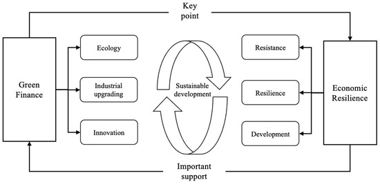
Figure 1.
Coupling mechanism of ER and GF.
First, the development system of ER covers three levels: resistance, resilience, and development. Improving the level of ER requires the participation of the government, the economy, medical care, research, science, technology, and culture [34,35]. We cannot separate any parts from the support of the financial system, and GF can play a crucial role in it. Resistance requires a stable social structure, production structure, and solid social foundation. The advancement of GF could catalyze the reformation of industrial systems, foster growth in public social undertakings, and bolster the enhancement of environmental responsibility [36]. At the same time, developing GF can also enhance the ability to prevent and defuse major risks and enhance the resilience of the economy aftershocks [37]. Regarding development power, GF can promote high-tech and green technology innovation, improve production efficiency, and transform the economy into a more advanced social development mode [38].
At the same time, the improvement of ER can enhance the stability and anti-risk ability of the economic system, prevent and defuse the impact of financial and economic risks, and thus provide a reliable economic environment for the development of GF. A stable economic environment can provide more favorable conditions for the development of the GF market, attract more investors and enterprises to participate in it, improve the liquidity and efficiency of the market, and thus promote the innovation of green financial products and the better transfer of green funds to green industries. In addition, the development of GF needs policy support and market cultivation, and a stable economic environment can provide a more powerful guarantee for policy implementation and market cultivation so that the development process of the GF market will be smoother and more sustainable [39].
2.2. ER and GF Index Evaluation System
Since ER and GF are multi-dimensional, a single indicator cannot fully reflect the other’s characteristics. Therefore, based on the research results of existing scholars, combined with the reliability and representativeness of data [23,40], this paper constructs an ER evaluation index system from three dimensions of ER: resistance, resilience, and development power. According to the development of GF in China and based on existing literature research [41], an evaluation index system based on five links of credit, securities, investment, insurance, and carbon finance is constructed. It comprehensively reflects the multi-dimensional characteristics of ER and GF (as shown in Table 1 and Table 2).

Table 1.
Green finance evaluation system.
Table 2.
Economic resilience evaluation system.
2.3. Methods
2.3.1. Entropy Value Method
The entropy method is utilized to compute and determine the weight of each evaluation index for the GF level and ER level, which are integrated through the weighted summation method. The calculation procedure comprises the following steps:
First, the raw data are processed with polar difference standardization method to consider the variances in the scale and positive/negative directions of each indicator.
Positive indicators:
Negative indicators:
The weight of the value of indicator d in the i-th provincial unit:
Calculation of the entropy value of the indicator:
Calculation of indicator weights:
Weighted summation calculation of population health level and economic development level:
where is the value of the d indicator for the i provincial unit. and are the minimum and maximum values of all provincial cells of the d-index, respectively. is the normalized value of the indicator d of the provincial unit i, m is the number of provincial cells, n is the number of indicators, is the entropy value of the d-index, is the weight of indicator d, and is the value of GF level and ER level for provincial unit i.
2.3.2. Coupling Coordination Degree Model
The term “coupling” has its roots in physics and signifies the existence of mutual interaction and influence between two or more systems or components. Subsequently, it has been extended to the realm of economics. The coupling level gauges the extent of correlation between systems, with greater coupling signifying stronger correlation and dependence between systems. Based on this, the coupling coordination degree model can more effectively capture the synergistic impact between systems [42,43,44].
The coupling degree model is described as follows:
stands for ER system, and stands for GF system. C is the coupling degree between ER and GF systems, and its value is between [0, 1]. C = 0 indicates that the systems are disordered; C = 1 means that the systems are completely ordered and form a benign resonance between the systems.
The coupling degree model needs to be improved in its ability to fully analyze the relationship between GF and ER. It does not indicate whether the two are mutually reinforced when the level of interaction is high or closely related when the level of interaction is low. It also cannot reflect the level of coordination between the two. Therefore, the coupled coordination degree model was introduced. This model can evaluate the level of coordinated development between GF and ER. The calculation is as follows:
D is the coupling coordination degree of the ER and GF systems, and its value is [0, 1]; T is the comprehensive development level of the ER and GF systems. are coefficients. Considering the interaction between the two systems, this paper believes that the two systems are equally essential and assign the same weight, so .
The classification of coupling coordination degree is shown in Table 3 [45].
Table 3.
Classification of coupling coordination degree.
2.3.3. Spatial Autocorrelation Model
This study employs the global Moran’s I index to evaluate the spatial correlation properties of the coupling degree between ER and GF in different provinces [46,47]. The formula used for calculation is as follows:
where and are the values of variables between neighboring provinces. is the data of the spatial weight matrix W. The space matrix is selected as 0-1 adjacency matrix, the neighbor rule is rook contiguity, and n is the number of regions. The value of I is [−1, 1]. If is positive, it means the space has a positive correlation; otherwise, it has a negative correlation.
Local spatial autocorrelation is conducted to analyze the spatial correlation between the coupling coordination degree of ER and GF, further explore the spatial nonequilibrium of local regions, and then analyze the spatial heterogeneity of the coupling coordination level of ER and GF among areas.
2.3.4. Kernel Density Estimation Method
Kernel density estimation is a non-parametric method commonly used to study the unbalanced distribution of regional variables [48,49]. It can analyze the spatial distribution characteristics of the research object according to the observed data. Usually, using frequency distribution maps can directly reflect the location, shape, ductility, and other information of the variable distribution. The expression of the kernel density estimation method is as follows:
“n” is the number of observed values; K (·) is the kernel density, the weight function. In this paper, we select the Epanechnikov kernel function [50]. “h” is bandwidth, and the smaller the bandwidth, the smaller the estimation deviation. According to Silverman’s rule of thumb, the optimal bandwidth is as follows:
Epanechnikov kernel function:
where u is the distance between an observation and the mean in the data set.
The position of the curve distribution indicates the degree of coupling coordination between ER and GF, while the height and width of the wave crest signify the inter-provincial differences in coupling coordination degree. The number of wave crests signifies the level of polarization within the sample. The ductility of the distribution indicates the extent of spatial differences between provinces with the highest level of coupling coordination and other provinces. Lastly, elongated right tail indicates increased difference.
2.3.5. Markov Transfer Matrix Analysis
Using kernel density estimation to test the evolution trend of regional variables is difficult to examine whether it is effective in terms of heterogeneity, nor can it reveal the evolution trend of regional variable distribution from the time dimension [51,52]. Markov transition matrix is an effective method to analyze whether there is “club convergence” in a region. When other conditions remain unchanged, the future state is only related to the present state and has nothing to do with the historical state. Traditional Markov transition matrix uses a Markov transition probability matrix with a probability value of of to abstract the state transition process of the whole thing. represents the one-step transition probability of the region belonging to type i in year t + 1 to type j, and its estimation method is as follows:
represents the sum of the provinces belonging to type i in a certain year in the observation period and transferred to type j in the lag period. is the sum of the number of provinces of type i in all years.
Based on the traditional Markov transfer matrix, we consider state transition probability analysis under different spatial lag types to reveal the influence of coupling coordination level between ER and GF in neighboring regions on dynamic regional evolution, which is used to analyze the convergence evolution characteristics of coupling coordination degree under the different backgrounds of neighboring areas [53,54,55,56]. An effective tool is also used to test whether there is “club convergence” in each region. If region i is adjacent to area j, the formula for calculating the Markov transfer matrix of the region i’s spatial lag type is
Lag represents the spatial lag operator; represents the coupling coordination degree between the ER of province i and GF. is the space lag weight. This paper adopts the adjacency principle to determine the spatial weight matrix: if provinces i and j are adjacent, its value is defined as 1; otherwise, it is 0. When , . The adjacency matrix is generated with GeoDa. The neighbor rule is rook contiguity.
2.4. Data Sources and Processing
In this paper, we will be focusing on the study period from 2011 to 2021. Our spatial scope covers 30 provinces, autonomous regions, and municipalities directly under the central government in mainland China, with the provincial administrative district as our spatial unit of study. We have yet to include Hong Kong, Tibet, Macao, and Taiwan in our study due to the lack of data available at this time. This paper’s numerical currency index data are based on 2010 and discounted by the corresponding price index to avoid the possible impact of price fluctuations on the empirical results. The data in this study mainly come from the China Statistical Yearbook, the statistical yearbooks of each region, and the China Stock Market and Accounting Research Database. We used the map data for our analysis, which was produced according to the standard map with review number GS (2020) 4619 from the Ministry of Natural Resources website. The base map remained unaltered during the process.
3. Results
3.1. ER and GF Development Level
Due to space constraints, only the data from 2011, 2013, 2015, 2017, 2019, and 2021 are listed here, and the specific results are shown in Table 4.
Table 4.
Comprehensive development level of GF and ER.
The finding illustrated in Figure 2 shows that the development of ER in various regions of China shows an apparent upward trend, with a significant increase in the growth rate, showing that China has achieved good results in increasing the level of ER in recent years. Regarding geographical distribution, the ER of the eastern region exceeds the national average, followed by the central area, and the western part comes in last. The east region has a sound foundation of geographical advantages, advantages in infrastructure construction, and human capital. At the same time, it is also the pioneer of the new policy. It has a sound foundation, strong impetus, and quick results.

Figure 2.
Development level of ER.
According to the data illustrated in Figure 3, GF development in China generally needed to be improved, displaying a fluctuating and declining trend before 2015, but has since exhibited a steady rise marked by consistent growth. From the perspective of regional distribution, the GF level of the eastern region is above the national average level. The western region ranked second and was overtaken by the central region after 2017. The result shows that geographical factors greatly influence the development of GF. The eastern region has natural advantages in green development due to its superior economic growth, capital allocation, and high-level talent. It is worth noting that the development of GF shows a fluctuating trend. We can see that GF’s development progress is not smooth, and there are still many obstacles.
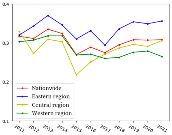
Figure 3.
Development level of GF.
3.2. Time Distribution Characteristics of RR and GF Coupling Coordination Degree
As shown in Figure 4, considering the temporal trends, the developmental trajectory of the coupling coordination measure between ER and GF in each province over the period of 2011–2021 can be bifurcated into two stages: the reluctant coordination stage (2011–2018) and the primary coordination stage (2019–2011). The two systems promote each other and coordinate with each other, and the coupling degree presents a steady upward trend on the whole. There was an increase of 13.8% from 0.535 in 2011 to 0.610 in 2021. After a slight decline in 2015, it continued to rise. The reason is that the development of GF stagnated in 2015, hindering the level of coupling and coordination among systems. Subsequently, the Overall Plan for the Reform of the Ecological Civilization System put forward in 2015 and the Guiding Opinions on Building a GF System put forward in 2016 have significantly promoted the development of GF and accelerated the level of coupling and coordination between the two systems. In general, during 2011–2014 and 2015–2021, the coupling of the two systems in the first four years resulted in lagging ER, while in the last seven years, mainly GF significantly lagged behind the development of ER and gradually widened the gap.
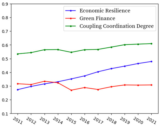
Figure 4.
Level of coupling coordination.
3.3. ER and GF Coupling Coordination Spatial Distribution Characteristics
This study classifies the coupling level into five distinct categories to render a clear visual representation of the coupling coordination degree of ER and GF in each province. We draw the spatial distribution of China’s coupling coordination degree between 2011 and 2021 using ArcGIS 10.2. Figure 5 displays the results of the selected time intervals.
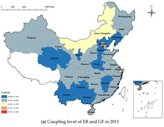
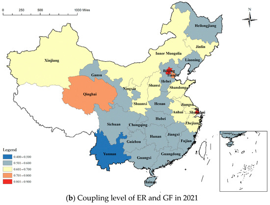
Figure 5.
Coupling level of ER and GF.
From the perspective of regional distribution, the regional differences between ER and GF coupling coordination degrees are apparent. While China’s ER and GF are improving, a significant gap exists between the eastern and central provinces. Taking 2021 as an example, the coupling coordination degree of Beijing and Shanghai is the highest, 8.67 and 8.34, respectively. Due to the comparative advantages of historical differences, location conditions, human capital, and other factors, the ER and GF of Beijing and Shanghai are much higher than those of other regions, making the coupling coordination degree far higher than the national average level of 0.609, reaching a good coordination level and approaching the advanced coordination level.
In contrast to the previous year, the overall level of the coupling coordination degree between ER and GF in the central and western provinces is relatively poor; most provinces are still in a state of reluctant coordination in the stage of excessive coordination, while Guangdong and Yunnan are on the verge of imbalance. The level of ER and GF development in the two provinces is relatively low, and there is potential for further progress in these areas. It is particularly worth pointing out that compared with 2011, Qinghai Province developed from the verge of imbalance to intermediate coordination in 2021, benefiting from the comprehensive implementation of a regional coordinated development strategy based on local conditions and giving full play to regional comparative advantages. To sum up, the spatial distribution of the coupling coordination degree between ER and GF presents an unbalanced situation between north and south and east and west.
3.4. Coordinated Spatial Autocorrelation Analysis of ER and GF
The range of values for global Moran’s I statistic is bounded between −1 and 1. If the value of I is positive, it indicates a positive correlation; a negative value implies a negative correlation, while a value of 0 indicates the absence of correlation. The larger the value, the smaller the overall difference. Table 5 shows the global Moran I test value of the coupling coordination degree of ER and GF from 2011 to 2021 which is calculated with StataSE. As shown in Table 5, Moran’s I index fluctuated around 0.5 from 2011 to 2021 and reached 6.40 and 6.90 in 2020 and 2021, showing a significant spatial correlation. The coupling coordination degree of national ER and GF shows a significant positive correlation; that is, there is an apparent spatial agglomeration, and the agglomeration degree has an upward trend, indicating that the integration of ER and GF shows a good development trend.
Table 5.
Global Moran’s I of coupling coordination degree.
To account for the limitations of the global Moran I test, which yields overly general results, our study employs the local Moran I test to assess the extent of regional spatial clustering in each area. This approach encompasses four agglomeration modes, namely “high-high,” “low-low,” “low-high,” and “high-low.” In particular, Figure 6 visually presents the local Moran scatter plot in 2011, 2015, 2018, and 2021, providing relevant insights into the clustering patterns over time.
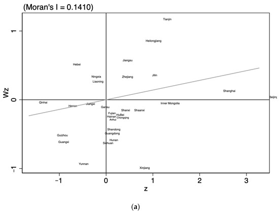
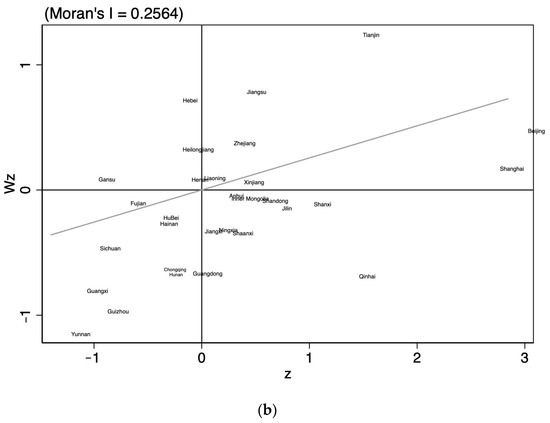
Figure 6.
Local Moran scatter plot of 2011 (a) and 2021 (b).
The scatter plot changed little from 2011 to 2021. The four plots in Figure 6 illustrate that the number of points in the first and third quadrants is noticeably higher than those in the second and fourth quadrants, pointing toward a substantial positive spatial correlation. In other words, there is a high similarity in the coupling coordination degree of both systems, and provinces, regions, and cities tend to cluster together. The coupling coordination degree of China’s ER and GF is mainly concentrated in the “H-H” and “L-L” clusters, with a noticeable spatial spillover effect.
Compared with 2011, in 2021, Beijing, Tianjin, Shanghai, and Zhejiang, located in the first quadrant, are located in the eastern coastal areas and have better geographical advantages. They have higher levels of GF development and ER development, as well as higher coupling coordination degrees, and their surrounding areas also have higher coupling coordination degrees, belonging to the “H-H” cluster area.
Located in the second quadrant, Hebei, Heilongjiang, Liaoning, Henan, Gansu, and other regions have low levels of ER and GF. It is worth highlighting that regions exhibiting low levels of coupling coordination are often hindered by relatively weak primary conditions. This implies that these regions struggle to develop interrelated systems despite their adjacency to regions with a high degree of coupling coordination. As a result, they need to improve their ability to leverage the synergistic benefits of their neighboring regions. It belongs to the “L-H” cluster area. Although the coupling coordination degree of Shanxi, Inner Mongolia, Jilin, Anhui, Shandong, Shaanxi, Qinghai, and Ningxia, which are located in the fourth quadrant, is higher than that of the surrounding areas, the coupling coordination degree of the adjacent regions is relatively low, which does not play a positive role of radiation driving, and belongs to the “H-L” agglomeration area with spatial heterogeneity. Regarding the specific regions located in the third quadrant of the local Moran scatter plot, it can be observed that they comprise Fujian, Jiangxi, Sichuan, Guizhou, Yunnan, Hubei, Guangxi, Hainan, Hunan, Guangdong, and Chongqing. These regions are characterized by relatively low degrees of coupling coordination, and the surrounding areas also exhibit a correspondingly low level of coupling coordination. Based on their mutual clustering patterns, these regions can be classified as belonging to the “LL” agglomeration group. The majority of these regions are situated in the northwestern and southwestern regions of China. The coupling and coordinated development of ER and GF are minimal. After ten years of development, some provinces have undergone quadrant changes depending on their development and the radiation effect of surrounding areas. For example, Henan and Shandong have changed from the third quadrant to the fourth quadrant, while some provinces have changed from the first to the second quadrant due to a lack of development impetus, such as Heilongjiang.
4. Dynamic Evolution Process and Prediction
4.1. Dynamic Evolution of ER and GF Coupling Coordination Degree
To further study the dynamic evolution trend of the coupled coordination degree of ER and GF over time and reveal the distribution characteristics of the coupling coordination degree of the two systems, this paper draws the kernel density curve of the coupled coordination degree of the country, eastern region, central region, and western region during 2011–2021 with StataSE, as shown in Figure 7a–d below.
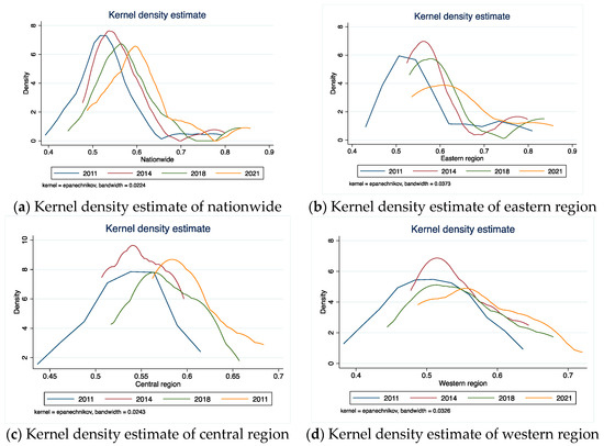
Figure 7.
Dynamic distribution of the coupling coordination degree between ER and GF.
Figure 7a depicts the temporal changes in the degree of coupling coordination between ER and GF across 30 provinces from 2011 to 2021. In general, the primary peak of the kernel density function is located to the right of its central point, and the entire distribution shifts toward the right over time. Furthermore, the peak height exhibits a pattern of an initial increase and a subsequent decline. The result indicates that the coupling coordination degree between ER and GF in most regions of China during the study period is medium to above and gradually improved. The range of variation distribution is gradually shortened, which indicates that although some areas are still ahead of the national level of coupling coordination, the gap between regions is narrowed, and the phenomenon of polarization is reduced. Viewing from the crest, the whole presents a “single-peak” distribution.
Figure 7b illustrates the temporal changes in the degree of coupling coordination between ER and GF, specifically in eastern China, from 2011 to 2021. The four curves depict a gradual shift toward the high-value side, and the peak of the nuclear density curve also shifts to the right with each passing year. These observations suggest a steady improvement in the coupling and coordination between ER and GF. Notably, the height of the primary peak decreased while the width of the curve notably shrank, and the nuclear density curve also trailed to the right, indicating a reduction in differences and an enhanced degree of coupling coordination in the eastern region.
Figure 7c showcases the temporal changes in the degree of coupling coordination between ER and GF in central China from 2011 to 2021. The kernel density curve exhibits a gentle peak, with the primary peak at the function’s midpoint. Over time, the curve shifts toward the right, suggesting a gradual improvement in the coupling coordination degree of ER and GF. The distribution interval of the kernel density curve remains relatively stable with insignificant changes. Moreover, the interval span of the curve is smaller than that observed in the eastern region, indicating a relatively low level of the coupling coordination degree in the central provinces.
Figure 7d presents the temporal changes in the degree of coupling coordination between ER and GF in western China from 2011 to 2021. The kernel density curve moves toward the right, and the primary peak gradually becomes gentle, forming a right skew. Compared to 2011, the kernel density curve in 2021 is located on the right side of the kernel density function. These findings suggest a gradual improvement in the coupling coordination degree of ER and GF in western provinces. However, an increasing trend of bifurcation and dispersion is observed, indicating a deviation or discrepancy in the coupling coordination degree across different regions in western China.
4.2. Spatio-Temporal Transfer Law of Coupling Coordination Degree between ER and GF
The kernel density function enables the depiction of the temporal evolution pattern of the coupling coordination degree between ER and GF across all provinces. However, it cannot judge the specific transfer law and the impact of neighboring provinces on their provinces’ coupling coordination degree level. Therefore, this paper uses MATLAB 2022 to calculate the traditional Markov transition matrix and further considers the geographical location and spatial effects.
4.2.1. Transfer Result of Coupling Coordination Degree Based on Traditional Markov Transfer Matrix
According to the conventional Markov transition matrix shown in Table 6, the diagonal elements represent the probability of a given region’s coupling coordination degree remaining relatively unchanged. On the other hand, the non-diagonal elements represent the probability of a transition occurring between different coupling levels. It is worth noting that these diagonal elements are crucial in determining the system’s overall stability. From 2011 to 2021, the coupling coordination degree of provinces did not show the “club convergence” phenomenon. Specifically, the probability of low-level, medium-low-level, medium-high-level, and high-level provinces maintaining the original state is greater than the probability of horizontal transfer, and it is easier to keep the original condition. However, in the long run, the likelihood of maintaining the initial state at low, medium-low, and medium-high levels decreased, and the probability of regressing to lower levels increased. However, the probability of maintaining the original level was still greater than the probability of horizontal transfer, and it was not easy to jump, showing an apparent path-dependent feature. Given the current situation, we must take targeted measures to improve the ER and GF in regions with relatively weak development. The coordinated development will bring the level of coupling and coordination to a higher level and prevent them from falling.
Table 6.
Traditional Markov transition matrix of coupling coordination degree.
4.2.2. Transfer Result of Coupling Coordination Degree Based on Spatial Markov Transfer Matrix
As can be seen from Table 7, under the same inter-period and different economic environments, the probability of a stable coupling coordination level or upward or downward transfer is different among provinces of the same type, showing a specific spatial dependence; that is, the coupling coordination degree of neighboring provinces will affect the coupling coordination level transfer probability of the province itself. Specifically, taking low-level provinces as an example, in the traditional Markov transfer probability matrix, the possibility of the low-level provinces maintaining the state is 91.9%. In contrast, when the influence of neighboring provinces is considered, the probability of the low-level provinces maintaining the state is 91.7%, 93.4%, 85.3%, and 100.0%, respectively. That is, neighboring provinces have a significant impact on their state changes. Among them, the low-level area is likely to progress to a higher level when the external environment is at a medium and high level through spatial effects. When the external environment is low, the path locking and “poverty trap” phenomenon is significant.
Table 7.
Spatial Markov transition matrix of coupling coordination degree.
We observe a space spillover effect whereby the degrees of coupling coordination between neighboring provinces influence each other. Specifically, when a province is adjacent to a region with a low coupling coordination degree, the likelihood of experiencing a downward transition in the state of the province increases. Conversely, when a province is adjacent to a region with a higher level of coupling coordination, the likelihood of an upward transition in the state of that province rises. For instance, over the short term, the upward transfer probabilities for middle- and low-level provinces show a steady upward trend, with values of 3.4%, 11.9%, 16.4%, and 60%, respectively, following improvements in the coupling coordination degree of neighboring provinces. Meanwhile, the probability of downward transfer for middle- to high-level provinces is 0%, 0%, 1.2%, and 2.8%, respectively. These observations suggest that the high-level areas’ spatial effect is more prominent than that of the low-level regions.
The spatial lag effect of neighboring provinces with lower coupling coordination degrees on the observed province is less negative than that of neighboring provinces with higher coupling coordination degrees. In the case of middle-to-low-level provinces with low-level neighboring provinces, the probability of a downward transition to a lower-level province is 8.3%, higher than the 8.1% observed with the traditional Markov transition matrix. This finding suggests that low-level neighbors are more likely to pull down the regional coupling coordination degree to a lower level. On the other hand, when neighboring provinces belong to middle-to-high or high-level regions, the likelihood of upward transition to middle-to-high-level provinces is 16.4% and 60%, respectively, higher than 13.3% in the traditional Markov transition matrix. This observation indicates that high-level neighbors contribute more to the upward transition of the regional coupling coordination degree.
Due to a development gap, the neighboring provinces with a large level difference have a more significant effect on the lower-level regions. That is, compared with the lower-level areas, the provinces themselves are more susceptible to the positive pulling effect of the higher-level neighbors, and the negative impact of the lower-level regions on the higher-level regions is weaker, which also shows that provinces that achieve high coupling coordination levels have stronger maintenance capabilities. Therefore, it is imperative to leverage the dominant role of economically advanced provinces, foster collaboration in narrowing the development disparity, facilitate the development of less developed regions through positive spillover effects, and establish a promotion paradigm for sustained growth.
5. Conclusions and Suggestions
Based on the scientific evaluation of ER and GF, this paper establishes a coupled coordination evaluation model of ER and GF. Taking 30 provinces, autonomous regions, and municipalities in mainland China as examples, the spatiotemporal distribution and dynamic evolution process of the coupled coordination of the two systems were explored using a spatial autocorrelation model, kernel density estimation, and Markov transfer matrix. The main conclusions are as follows:
(1) The degree of coupling coordination between ER and GF has gradually improved and gained momentum. While ER has continuously bolstered, the development of GF has exhibited fluctuating growth. The coordinated and integrated development of both systems is mainly driven by ER. Nonetheless, the widening development gap between them poses a challenge to their continuing coordinated development.
(2) High levels of coupling coordination are primarily concentrated in regions along the eastern coast, while low levels of coupling coordination are distributed across various regions, mainly in the western part of the country. Despite the nationwide improvement, there is still a significant polarization in terms of the degree of coupling coordination, and the discrepancy between the eastern and western regions continues to widen.
(3) The coupling coordination levels of ER and GF have a significant spatial correlation. The coupling coordination levels between neighboring provinces will influence each other, and the higher-level region more obviously drives the lower-level region. The internal coupling coordination degree of each area does not show the “club convergence” phenomenon, and the convergence process is not independent of time and space. In particular, when a considerable disparity exists between adjacent provinces, the development gap may impede the synergic effect derived from the positive interaction among proximal regions.
Drawing on the above research outcomes, the ensuing recommendations are as follows:
(1) Building regional linkage and promoting regional coordinated development is necessary. Lower-level regions should strengthen exchanges and cooperation with developed areas, actively learn from the advanced experience of developed regions, and make use of the trickle-down effect of the ER and GF coupling coordination degree to establish long-term and effective cooperation and a collaborative governance mechanism between high-level coastal regions and lower-level inland regions. It is also recommended to set a central city cluster and radiate the development of low-level areas in points and regions. It is necessary not only to actively promote the benign positive diffusion from the region with a high coupling coordination degree to the region with a low level in eastern China but also to promote the balanced development of a regional economy. Based on effective risk control, it is necessary to prevent the negative spatial spillover effect from aggravating the spread of the crisis to maintain the sustainable development of a regional economy.
(2) The government must strengthen modernization, improve infrastructure, and upgrade industrial models. It should also deepen financial reform and accelerate urban financial development in order to alleviate the financial difficulties faced in the process of technological innovation so as to promote urban technological progress and industrial upgrading. To match the policy promotion mode of GF with the industrial structure, government departments should do an excellent job of guidance. Regarding policy matching, we should grasp the heat of market clearance, minimize the cyclical fluctuation of the policy effect, and it is necessary to secure the durability of policy efficacy over the long term. It is recommended that the central government reinforce primary fiscal outlays, expedite the development of infrastructural facilities such as education and healthcare, and enhance the technological advancement of public services.
(3) Strengthening technological innovation, cultivating technical talents, and promoting quality development are crucial. We should vigorously introduce and cultivate scientific and technological personnel, build a high ground for human innovation, and provide personnel support for the innovative development of scientific and technical finance and advanced manufacturing. For fostering the growth and advancement of GF and advanced manufacturing, it is proposed that the government concentrate on addressing the technical challenges confronted by major progressive manufacturing enterprises, considering the specific advantages and requirements of regional industrial development. The innovative development of advanced manufacturing enterprises can be accelerated by effectively harnessing the influential and dynamic role of science and technology finance in the area of scientific and technological innovation and outcome transformation.
6. Limitations and Future Research
Due to limited data availability and imperfect knowledge, this study has some limitations. For example, the coupling coordination degree evaluation model must be further optimized. More indicators should be considered, such as green consumption and other aspects of life. In addition, further empirical analysis is needed to analyze the interactions between GF and ER. With data availability and in-depth research, these issues will be further explored in our future work.
Author Contributions
Conceptualization, J.Z.; data curation, X.H.; methodology, J.Z.; resources, J.Z.; supervision, S.Z.; visualization, Z.Z.; writing—original draft, J.Z.; writing—review and editing, J.Z. and S.Z.; software, C.J. All authors have read and agreed to the published version of the manuscript.
Funding
This research was funded by the Graduate Student Innovation Fund of the Anhui University of Science and Technology, grant number “2022CX2150”.
Acknowledgments
The authors wish to thank the three reviewers for their helpful comments and suggestions.
Conflicts of Interest
The authors declare no conflict of interest.
References
- Huang, S.; Xu, L.Q. The driving factors of green finance development: Evidence from China. J. Clean. Prod. 2019, 233, 882–890. [Google Scholar]
- Huang, S.; Zhang, Y.; Ma, B. Social interconnection and the development of green finance: A perspective from China. Technol. Forecast. Soc. Chang. 2019, 148, 119697. [Google Scholar]
- Terpstra, T.; Olsthoorn, M.; Koppenjan, J. Resilience in the face of a crisis: A case study of flood-affected firms. J. Risk Res. 2020, 23, 572–587. [Google Scholar]
- Reggiani, A.; De Graaff, T.; Nijkamp, P. Resilience: An Evolutionary Approach to Spatial Economic Systems. Netw. Spat. Econ. 2002, 2, 211–229. [Google Scholar] [CrossRef]
- Paton, D.; Johnson, D. Disasters and Communities: Vulnerability, Resilience and Preparedness. Disaster Prev. Manag. 2001, 10, 270–277. [Google Scholar] [CrossRef]
- Wildavsky, A.B. Searching for Safety; Routledge: London, UK, 1988; pp. 118–124. [Google Scholar]
- Barnett, J. Adapting to Climate Change in Pacific Island Countries: The Problem of Uncertainty. World Dev. 2001, 29, 977–993. [Google Scholar] [CrossRef]
- Thomalla, F.; Downing, T.; Spanger-Siegfried, E.; Han, G.; Rockström, J. Reducing Hazard Vulnerability: Towards a Common Approach between Disaster Risk Reduction and Climate Adaptation. Disasters 2006, 30, 39–48. [Google Scholar] [CrossRef]
- Evans, J.P. Resilience, Ecology and Adaptation in the Experimental City. Trans. Inst. Br. Geogr. 2011, 36, 223–237. [Google Scholar] [CrossRef]
- Van Bergeijk, P.A.G.; Brakman, S.; Van Marrewijk, C. Heterogeneous economic resilience and the great recession’s world trade collapse. Pap. Reg. Sci. 2017, 96, 3–13. [Google Scholar] [CrossRef]
- Davies, S. Regional resilience in the 2008-2010 downturn: Comparative evidence from European countries. Camb. J. Reg. Econ. Soc. 2011, 4, 369–382. [Google Scholar] [CrossRef]
- Brakman, S.; Garretsen, H.; Van Marrewijk, C. Regional resilience across Europe: On urbanisation and the initial impact of the Great Recession. Camb. J. Reg. Econ. Soc. 2015, 8, 309–312. [Google Scholar] [CrossRef]
- Briguglio, L.; Cordina, G.; Farrugia, N.; Vella, S. Conceptualizing and Measuring Economic Resilience. Building the Economic Resilience of Small States. 2006, pp. 265–288. Available online: https://www.researchgate.net/publication/335930167_Conceptualising_and_measuring_economic_resilience (accessed on 12 April 2023).
- Martin, R.; Sunley, P.; Gardiner, B.; Tyler, P. Regional economic resilience, hysteresis and recessionary shocks. J. Econ. Geogr. 2012, 12, 1–32. [Google Scholar] [CrossRef]
- Oprea, F.; Onofrei, M.; Lupu, D.; Vintila, G.; Paraschiv, G. The determinants of economic resilience. The case of eastern european regions. Sustainability 2020, 12, 4228. [Google Scholar]
- Xu, Y.S.; Warner, M.E. Understanding employment growth in the recession: The geographic diversity of state rescaling. Camb. J. Reg. Econ. Soc. 2015, 8, 205–225. [Google Scholar] [CrossRef]
- Martin, R.; Sunley, P.; Gardiner, B.; Coombes, M.; Green, A. How regions react to recessions: Resilience and the role of eco-nomic structure. Reg. Stud. 2016, 50, 561–585. [Google Scholar] [CrossRef]
- Brown, L.; Greenbaum, R.T. The Role of Industrial Diversity in Economic Resilience: An Empirical Examination Across 35 Years. Urban Stud. 2017, 54, 1322–1339. [Google Scholar] [CrossRef]
- Martin, R.; Sunley, P.; Tyler, P. Local Growth Evolutions: Recession, Resilience and Recovery. Camb. J. Reg. Econ. Soc. 2015, 8, 205–225. [Google Scholar] [CrossRef]
- Desalegn, G.; Tangl, A. Enhancing Green Finance for Inclusive Green Growth: A Systematic Approach. Sustainability 2022, 14, 7416. [Google Scholar] [CrossRef]
- Salazar, J. Environmental Finance: Linking Two Worlds. Financial Innovations for Biodiversity. Bratislava 1998, 1, 2–18. [Google Scholar]
- Cowan, E. Topical Issues in Environmental Finance; Asia Branch of the Canadian International Development Agency (CIDA): Toronto, ON, Canada, 1999. [Google Scholar]
- Lee, J.W. Green finance and sustainable development goals: The case of China. J. Asian Financ. Econ. Bus. 2020, 7, 577–586. [Google Scholar] [CrossRef]
- Dikmen, N.; Tutar, M. Green finance and sustainable economic growth: Evidence from selected developing countries. Environ. Sci. Pollut. Res. 2020, 27, 35081–35094. [Google Scholar]
- He, Y.; Liu, J. Innovation diffusion in green finance: Evidence from China. J. Clean. Prod. 2021, 285, 125170. [Google Scholar]
- Labatt, S.; White, R. Environmental Finance: A Guide to Environmental Risk Assessment and Financial Products; John Wiley & Sons, Inc.: Toronto, ON, Canada, 2002; pp. 3–12. [Google Scholar]
- Zhou, X.; Tang, X.; Zhang, R. Impact of Green Finance on Economic Development and Environmental Quality: A Study Based on Provincial. Environ. Sci. Pollut. Res. 2020, 27, 19915–19932. [Google Scholar] [CrossRef] [PubMed]
- Wang, E.; Hong, D.; Chang, Y.; Qiao, Y. The influence of green insurance on corporate environmental protection behavior: Evi-dence from China. J. Clean. Prod. 2021, 311, 127808. [Google Scholar]
- Li, C.; Chen, Z.; Wu, Y.; Zuo, X.; Jin, H.; Xu, Y.; Zeng, B.; Zhao, G.; Wan, Y. Impact of Green Finance on China’s High-Quality Economic Development, Environmental Pollution, and Energy Consumption. Front. Environ. Sci. 2022, 10, 2205. [Google Scholar] [CrossRef]
- Zhang, Z.; Duan, H.; Shan, S.; Liu, Q.; Geng, W. The impact of green credit on the green innovation level of heavy-polluting enterprises—Evidence from China. Int. J. Environ. Res. Public Health 2022, 19, 650. [Google Scholar] [CrossRef]
- Liu, S.; Xu, R.X.; Chen, X.Y. Does green credit affect the green innovation performance of high-polluting and energy-intensive enterprises? Evidence from a quasi-natural experiment. Environ. Sci. Pollut. Control. Ser. 2021, 28, 65265–65277. [Google Scholar] [CrossRef]
- Lin, B.; Huang, W. Does green finance improve regional economic and energy structure? Evidence from China. J. Clean. Prod. 2021, 279, 123740. [Google Scholar]
- Yao, D.; Wang, X.; Yao, Y. The Impact of Green Finance Development on the Macro-Economic Resilience in China. J. Shandong Univ. Financ. Econ. 2023, 35, 13–26. [Google Scholar]
- Li, R.; Li, F.; Li, Y.; Wang, X.; Wang, X. Resilience Evaluation of Resource-Based Cities in China Using a Hierarchical System Stability Analysis Model. J. Clean. Prod. 2021, 317, 128297. [Google Scholar]
- Hu, B.; Wang, X.; Liu, Y.; Fu, H.; Zhang, X. Does Green Finance Help Mitigate Climate Change? A Case Study of the China BRICs Countries. J. Clean. Prod. 2019, 228, 1546–1557. [Google Scholar]
- Li, Y.; Xie, Q. Research on the Influence of Ecological Restoration on Green Finance: Take Water Source Protection Projects in the Minjiang River Basin as an Example. J. Clean Prod. 2019, 236, 117490. [Google Scholar]
- Wang, T.; Duan, C.; Lu, Z. The Relationship between Green Finance and Regional Ecological Conservation: Evidence from China. J. Clean. Prod. 2021, 319, 128322. [Google Scholar]
- Agrawal, S.; Chatterjee, R. Green finance: Challenges and opportunities for innovation. J. Open Innov. Technol. Mark. Complex. 2019, 5, 4. [Google Scholar]
- Tao, R.; Zhou, S. Is There a Positive Relationship between Green Finance and Economic Growth? An Empirical Study of the Belt and Road Initiative Based on the Panel Data. Environ. Sci. Pollut. Res. 2020, 27, 35697–35708. [Google Scholar]
- Xu, X.; Wang, M.; Wang, M.; Yang, Y.; Wang, Y. The Coupling Coordination Degree of Economic, Social and Ecological Resil-ience of Urban Agglomerations in China. Int. J. Environ. Res. Public Health 2023, 20, 413. [Google Scholar] [CrossRef]
- Zhang, J.; Zhang, S.; Zhang, Y. Evaluation of the Effect of Green Finance in Promoting Green Technology Innovation: A Two-Stage DEA Model. J. Taiyuan City Vocat. Tech. Coll. 2022, 256, 185–187. [Google Scholar]
- Yang, Y.; Wang, R.; Tan, J. Coupling Coordination and Prediction Research of Tourism Industry Development and Ecological Environment in China. Discret. Dyn. Nat. Soc. 2021, 2021, 6647781. [Google Scholar] [CrossRef]
- Sun, L.; Wang, Z.; Yang, L. Research on the Dynamic Coupling and Coordination of Science and Technology Innovation and Sustainable Development in Anhui Province. Sustainability 2023, 15, 2874. [Google Scholar] [CrossRef]
- Hou, C.; Chen, H.; Long, R. Coupling and Coordination of China’s Economy, Ecological Environment and Health from a Green Production Perspective. Int. J. Environ. Sci. Technol. 2022, 19, 4087–4106. [Google Scholar] [CrossRef]
- Tang, H.; Chen, Y.; Ao, R.; Shen, X.; Shi, G. Spatial-Temporal Characteristics and Driving Factors of the Coupling Coordination between Population Health and Economic Development in China. Sustainability 2022, 14, 10513. [Google Scholar] [CrossRef]
- Cheng, M.; Wei, Y.M.; Fan, L.W. Spatial-temporal heterogeneity of the coupling relationship between green finance and energy transition in China. Energy Policy 2020, 137, 111091. [Google Scholar]
- Moran, P.A.P. Notes on Continuous Stochastic Phenomena. Biometrika 1950, 37, 17–23. [Google Scholar] [CrossRef]
- Dai, J.; Liu, Y.; Chen, J.; Liu, X. Fast Feature Selection for Interval-Valued Data through Kernel Density Estimation Entropy. Int. J. Mach. Learn. Cybern. 2020, 11, 2607–2624. [Google Scholar] [CrossRef]
- Mnatsakanov, R.; Sarkisian, K. Varying Kernel Density Estimation on Statist. Probab. Lett. 2012, 82, 1337–1345. [Google Scholar] [CrossRef]
- Rosenblatt, M. Remarks on Some Nonparametric Estimates of a Density Function. Ann. Math. Stat. 1956, 27, 832–837. [Google Scholar] [CrossRef]
- Kaijser, T. On Markov Chains Induced by Partitioned Transition Probability Matrices. Acta Math. Sin. 2011, 27, 441–476. [Google Scholar] [CrossRef]
- Kaijser, T. A Limit Theorem for Partially Observed Markov Chains. Ann. Probab. 1975, 3, 677–696. [Google Scholar] [CrossRef]
- Wang, S.; Gao, S.; Huang, Y.; Shi, C. Spatiotemporal Evolution of Urban Carbon Emission Performance in China and Predic-tion of Future Trends. J. Geogr. Sci. 2020, 30, 757–774. [Google Scholar] [CrossRef]
- Han, Y.; Jia, H. Simulating the spatial dynamics of urban growth with an integrated modeling approach: A case study of Foshan, China. Ecol. Model. 2017, 353, 107–116. [Google Scholar] [CrossRef]
- Kaijser, T. On Convergence in Distribution of the Markov Chain Generated by the Filter Kernel Induced by a Fully Dominated Hidden Markov Model. Dissertationes Math. 2016, 514. [Google Scholar] [CrossRef]
- Rey, S.J. Spatial Empirics for Economic Growth and Convergence. Geogr. Anal. 2001, 33, 195–214. [Google Scholar] [CrossRef]
Disclaimer/Publisher’s Note: The statements, opinions and data contained in all publications are solely those of the individual author(s) and contributor(s) and not of MDPI and/or the editor(s). MDPI and/or the editor(s) disclaim responsibility for any injury to people or property resulting from any ideas, methods, instructions or products referred to in the content. |
© 2023 by the authors. Licensee MDPI, Basel, Switzerland. This article is an open access article distributed under the terms and conditions of the Creative Commons Attribution (CC BY) license (https://creativecommons.org/licenses/by/4.0/).