Study on Vertical Load Distribution of Pile Group–Liquefied Soil System under Horizontal Seismic Environment

Abstract

The dynamic responses of pile–liquefied composite soils are complex, and the bearing capacities of single piles or pile groups in liquefiable soils remain unclear. For friction piles, the friction resistance determines the vertical bearing capacity of the pile. In a pile–soil system, it is very important to study the friction resistance changes in the pile during vibration. Based on a shaking table test, this study investigated the vertical bearing capacity of a pile foundation–liquefied soil system under simulated horizontal seismic forces, using the MIDAS GTS software. The load borne by the top of the pile was studied under a horizontal earthquake with a certain vertical load, different pile spacings, and different vibration times, along with the cumulative coefficient CCPF of the pile side friction. The distributions of the CCPF along the pile body of a single pile and pile groups with different pile spacings were analyzed at different vibration times. It was found that the CCPF intuitively reflected the distribution law of the pile side friction during vibration. When the CCPF at the bottom of the pile was equal to 1, the load on the top of the pile was equal to the average value of the total load. When the CCPF at the bottom of the pile was less than 1, the load on the top of the pile was less than the average value of the total load. When the CCPF at the bottom of the pile was greater than 1, the load on the top of the pile was greater than the average of the total load.

1. Introduction

In recent years, earthquakes have occurred frequently all over the world, and the resulting disasters are becoming more and more serious. There are many causes of disasters. However, due to the effects of an earthquake’s force, damaged pile foundations, along with decreases in bearing capacity, are undoubtedly some of the most important resulting disasters. For this reason, the topic of pile–soil dynamic interaction has been gradually valued and studied by relevant scholars in recent years. However, this subject involves many factors, such as pile groups, the properties of the soil around piles, and the infinity of the underlying foundation soil, as well as cross-research of the structural dynamics and soil dynamics, which makes the research of this subject very complex; thus, the relevant research progress is relatively slow.

The study of the dynamic interaction between liquefied soil and pile foundations is mainly based on p–y curves. Zhang Chongwen et al. [1], Huang Qunxian et al. [2], and others regarded the pile–soil interaction as a nonlinear relationship, using ANSYS analysis software, and used spring elements to simulate the lateral force of the pile foundation. Yang Weilin et al. [3] established a one-dimensional wave model to simulate the seismic action, and extended this to two-dimensional and three-dimensional models to study the pier–pile group–soil interaction. Additionally, the influence of different models on the peak acceleration of the pile foundation was obtained. Su Jingbo et al. [4] and others established a nonlinear contact finite element model of pile–soil interaction by using the Newmark theory. They conducted relevant numerical simulation research on pile–soil interaction and obtained the sensitivity calculation formula of different soil parameters to the displacement of liquefiable sand. Rahmani et al. [5] used a numerical model, developed in the GiD + OpenSees interface V2.6.0, to investigate the effect of DSM improvement with a grid pattern on foundation settlement and EPWP generation. The results also indicated that the grid wall spacing, diameter of the columns, soil relative density, and shear modulus ratio between the DSM columns and the enclosed soil play a vital role in liquefaction occurrence and volumetric strains. Maleki et al. [6] used numerical simulation to study the dynamic characteristics of deep foundation pits during earthquakes, and the research results showed that the dynamic performance of a deep excavation during a seismic event is greatly influenced by the characteristics of the input motion (fundamental frequency, amplitude, and duration), as well as the properties of geo-materials.

In addition, in terms of shaking table research, Wu Xiaoping et al. [7] carried out relevant tests on a pile–model soil system by means of a shaking table test, and obtained the response of the upper structure and soil properties at different locations to the pile body strain. Wang Jianhua et al. [8] carried out shaking table tests on a pile foundation–saturated sand system with different relative densities, obtained the p–y curve to evaluate the horizontal bearing capacity of the pile foundation, and presented the change trend of the hole pressure ratio. Qi Chunxiang et al. [9] proposed that it is generally assumed that the lateral resistance P of the soil mass and displacement y of the foundation are typical nonlinear relationships. Zhao Chenggang et al. [10] and others summarized three different calculation methods for soil liquefaction by referring to the change in pile stress. Li Yurun et al. [11] and others carried out further theoretical research on p–y curves, based on shaking table tests, and put forward an optimized p–y curve method. Overseas, Amar et al. [12], Paramasivam et al. [13], Al-Isawi et al. [14], Nadarajah et al. [15], and other scholars have carried out relevant research on pile–liquefied soil dynamic interaction and reached corresponding conclusions.

A large number of studies have studied pile–soil dynamic interaction based on the horizontal dynamic characteristics, but there have been few studies on the vertical bearing capacity of pile foundations under dynamic loads. The two-stage analysis method in the current standard is applicable to low pile caps. In two-stage analysis, the pile foundation monitoring calculation is divided into two stages: the earthquake stage and the post-earthquake stage. In the earthquake stage, the pile body is affected by the earthquake force, and there is already a liquefaction area in the soil. According to the fact that most of the water spraying and gushing out lags behind the earthquake, it is generally considered that the liquefaction area will not have developed near the top of the pile in this stage. Considering that the impact on the transverse bearing capacity is not large, the liquefaction impact can be ignored in the seismic calculation, and the monitoring of the bearing capacity of the pile foundation is the same as that of the non-liquefied soil. The pile body does not act on seismic force in the post-earthquake stage. The vertical bearing capacity of the pile foundation after liquefaction is monitored under a static load. It is almost impossible to determine the bearing capacity of the pile foundation at different vibration times using a model test. Based on a laboratory model test [16], through a comprehensive understanding and analysis of relevant research at home and abroad, this paper established an intuitive and clear mathematical model by using the three-dimensional finite element analysis software MIDAS GTS of the geotechnical engineering specialty, and selected reasonable numerical simulation parameters. The vertical bearing characteristics of a pile foundation under simulated seismic force using the same conditions were analyzed, and were tested in a laboratory.

2. Determination of Relevant Conditions for Numerical Simulation

2.1. Constitutive Relationship of Soil Mass

The constitutive relationship model, established based on elastic–plastic theory, considers two aspects of the soil [17]: elastic deformation that can be restored, and plastic deformation that cannot be restored. They are calculated using two deformation theories to reflect the working characteristics of the soil. The plastic theory calculation for soil usually involves yield surface theory, the flow law, and strengthening theory to determine the conditions, direction, and magnitude of the plastic strain increment in the soil. The earliest constitutive relationship model proposed based on plastic theory was based on the D–P yield criterion for elastic–plastic constitutive relations. A large number of scholars’ practical studies have shown that the D–P yield criterion has consistency in fitting soil deformation and failure and Mohr–Coulomb. At the same time, it also adopts the generalized von Mises yield condition, and has achieved good results in soil elastic–plastic dynamic analysis. The expression is:

$$f\left(p,\sqrt{J_2}\right)=3\sqrt{J_2}\alpha p-k=0$$

(1)

According to the relevant flow laws, these are the following expressions:

$$d{\epsilon }_{ij}^p=d\lambda \frac{\partial f}{\partial {\sigma }_{ij}}$$

(2)

$$“\mathrm{H}” \mathrm{is} \mathrm{the} \mathrm{hardening} \mathrm{parameter} d\lambda =\frac{H_{ij}d{\epsilon }_{ij}}{H}$$

(3)

$$H_{ij}=-3\alpha K{\delta }_{ij}+G\frac{1}{\sqrt{J_2}}{s}_{ij}$$

(4)

$$\overline{H}=9{\alpha }^{2}K$$

(5)

$$J_2=\frac{1}{6}\left[{\left({\sigma }_x-{\sigma }_y\right)}^2+{\left({\sigma }_y-{\sigma }_z\right)}^2+{\left({\sigma }_z-{\sigma }_x\right)}^2\right]+{\tau }_{xy}^2+{\tau }_{yz}^2+{\tau }_{zx}^2$$

(6)

The expression of the D–P constitutive relationship model is:

$$d{\sigma }_{ij}=D_{ijkl}^{ep}d{\epsilon }_{kl}=[D_{ijkl}^e-D_{ijkl}^p]d{\epsilon }_{kl}$$

(7)

The elastic–plastic matrix is:

$$D_{ijkl}^{ep}=(K-\frac{2}{3}G){\delta }_{ij}{\delta }_{kl}+2G{\delta }_{ik}{\delta }_{jl}-\frac{H_{ij}{H}_{kl}}{H+G}$$

(8)

where G is the shear modulus, and K is the bulk elastic modulus.

In the principal stress space, the standard yield surface of the D–P model is a conical surface, as shown in Figure 1. The shape of the yield surface on the conical surface is very similar to that of the Mohr–Coulomb model. According to the expression of the D–P model, the basic control parameters are the elastic modulus, density, internal friction angle, Poisson’s ratio, and soil cohesion, along with the introduction of the effect of hydrostatic pressure. The plastic behavior curve is shown in Figure 2.

Based on the characteristics of the soil in the shaking table tests, the D–P elastic–plastic model was selected as the constitutive relationship of the soil in the numerical analysis in this article, providing an important theoretical basis for the analysis of soil characteristics under the joint action of the pile, soil, and pile cap.

2.2. Model Boundary Conditions

In numerical models, different action forms have different boundary treatment methods. The theory and control of boundary conditions under dynamic loads are very complex, representing popular and difficult topics in current research. The viscoelastic artificial boundary proposed by Deesk [18] basically solves this problem, and can accurately simulate the radiation damping of the soil at the boundary and the elastic recovery of the foundation. This method is realized by adding parallel linear springs and viscous dampers to the boundary to absorb the waves scattered on the interface. In this study, the viscoelastic artificial boundary was used.

The shear wave velocity of the upper soil was set to 60 m/s, and the P wave velocity was set to 130 m/s. The shear wave velocity of the lower soil was set to 280 m/s, and the P wave velocity was set to 700 m/s. The nodes on the model boundary were selected, and springs and dampers on the nodes on the model boundary were set to generate the viscoelastic boundary, as shown in Figure 3.

2.3. Damping Setting

Currently, the most widely used theory is proportional damping, where the damping force can be expressed as $\mu \left\{D\right\}\left\{\dot{\epsilon }\right\}$. It is proportional to the stiffness matrix of the element, making it easy to obtain the damping matrix in dynamic calculations. By orthogonalizing the mass and stiffness matrices, it can be conveniently represented as a damping matrix. [M] and [K] represent the mass and stiffness matrices, respectively, and the stiffness matrix representation is expressed by (9):

$$\left[C\right]=\alpha \left[M\right]+\beta \left[K\right]$$

(9)

$$\alpha =\frac{2{\omega }_i{\omega }_k}{{\omega }_i+{\omega }_k}\zeta ,\hspace{1em}\beta =\frac{2}{{\omega }_i+{\omega }_k}\zeta$$

(10)

where $\zeta$ is the damping ratio of the system, and ${\omega }_i$ and ${\omega }_k$ are the frequency vibration rates of the two modes of the system.

Rayleigh damping is based on the theory of proportional damping, combined with the characteristics of soil under dynamic action, to reduce the uncertainty of stiffness-proportional damping in higher-order vibration modes. It is very practical for the application of soil in earthquake engineering, and is extremely convenient for calculation.

In the MIDAS GTS program, damping types are mass-proportional, stiffness-proportional, and Rayleigh-type. Rayleigh damping is often used in entity analysis; therefore, Rayleigh damping was used in the calculation model. The mass and stiffness factors are a₀ = 0.026 and a₁ = 0.401 [19], respectively.

2.4. Contact Unit Selection

The structures in the soil studied in this paper were a pile and a cap. The rigidity of the pile and cap is much higher than that of the soil. Under the action of external force, when the soil is in the plastic state, the pile and cap are still in the elastic stage. Additionally, this paper mainly studied the dynamic vertical bearing characteristics of the pile foundation system, without considering the damage in the horizontal direction; therefore, it was appropriate to adopt the linear elastic model for the pile and cap to meet the test requirements, which also allowed the convergence speed of the calculation to be greatly improved.

In model analysis, there will be incongruous deformation between the two materials at the contact surface of different materials (there are obvious differences in stiffness). In addition, soil is a typical nonlinear material, which will show obvious nonlinearity, even if there is small deformation. Therefore, on the contact surface between the pile and soil, due to the inconsistent deformation, it is impossible for the pile to transmit all the force to the soil, meaning that part of the energy is lost. In order to correctly reflect the interaction of the pile–soil system under dynamic action, a Goodman contact unit surface, which can generate individual deformation, was set between the pile, soil, and bearing cap. In this paper, the modified Goodman element was adopted, and the damping factor was considered, which further simulated the energy loss on the contact surface of the pile, soil, and cushion cap.

The contact element has no thickness and mass. The Goodman element was modified in this study to consider the damping or energy loss at the interface of pile-soil:

$$D=\left[\begin{array}{ccc}{k}_n& 0& 0\\ 0& k_s& 0\\ 0& 0& k_s\end{array}\right]$$

(11)

$$k_s=\frac{\partial \tau }{\partial {\omega }_s}=k_1{\gamma }_w(\frac{{\sigma }_n}{P_a}{)}^n(1-\frac{R_f\tau }{{\sigma }_n\mathit{tan}\delta }{)}^2$$

(12)

where $k_n$ is the normal stiffness, $k_s$ is the shear stiffness, $\delta$ is the friction coefficient between soil and structure, ${\gamma }_w$ is the gravity of water, $k_1$, n and $R_f$ are nonlinear parameters of soil, ${\sigma }_n$ is the normal stress, and $P_a$ is the standard atmospheric pressure.

The damping term in Equation (9) will be added to the above modified Goodman element in the dynamic calculation. Thus, the shear strain of the soil around the pile presents a nonlinear change. This can make the contact element perform a nonlinear change. The Goodman element between pile and soil is set as the following relationship, to reflect the deformation and interaction of pile and soil:

$$[C]=\frac{\lambda }{\omega }[D]$$

(13)

where $\lambda$ is wavelength, and $\omega$ is frequency.

The relevant parameters of the contact unit are shown in

Table 1. Parameters of various contact elements.

	Pile–Soil	Cap–Soil	Pile–Cap
Normal stiffness Kn (kPa)	8000	8000	10,000
Shear stiffness Ks (kPa)	1400	283	1500
Internal friction angle (o)	29	29	—
Cohesion (kPa)	78	17	—

. Figure 4 shows the contact elements between the soil and structures.

2.5. Seepage Theory and Soil Consolidation

This simulation used Biot consolidation theory. The soil unit is shown in Figure 5. The momentum equation is as follows:

$$\begin{array}{c}\frac{\partial {\sigma }_x}{\partial x}+\frac{\partial {\tau }_{xy}}{\partial y}+\frac{\partial {\tau }_{zy}}{\partial z}+\rho \ddot{u}=0\\ \frac{\partial {\sigma }_y}{\partial y}+\frac{\partial {\tau }_{zy}}{\partial z}+\frac{\partial {\tau }_{xy}}{\partial x}+\rho \ddot{v}=0\\ \hspace{1em}\hspace{1em}\hspace{1em}\hspace{1em}\frac{\partial {\sigma }_z}{\partial z}+\frac{\partial {\tau }_{xz}}{\partial x}+\frac{\partial {\tau }_{yz}}{\partial y}+\rho \ddot{w}-\rho g=0\end{array}$$

(14)

The relationship among the total stress, pore pressure, and effective stress is analyzed according to the principle of effective stress:

$$\left\{\sigma \right\}=\left\{{\sigma }^{\prime }\right\}+\left\{p\right\}$$

(15)

The stress–strain relationship can usually be expressed as:

$$\left\{d{\sigma }^{\prime }\right\}=\left[D^{ep}\right]\left\{d\epsilon \right\}$$

(16)

where $\left[D^{ep}\right]$ is the elastic–plastic matrix of the soil and the strain increment in the soil skeleton.

2.6. Mesh

In finite element method numerical modeling, the establishment of computational grids can be achieved through software-free partitioning generation, scanning generation, mapping generation, and the extension of two-dimensional methods to three-dimensional methods. The mesh of solid elements is generally tetrahedral or hexahedral. A tetrahedral element mesh is easy to partition, but its accuracy is not high enough. The calculation accuracy of a hexahedral mesh is relatively accurate, but it is difficult to divide the mesh. The more regular the model, the faster the calculation speed and the higher the accuracy. If circular piles are used in the calculation, the grid division at the interface between the piles and soil is prone to distortion. Although tetrahedral elements can be used for the division, the resulting grid is relatively chaotic, making it difficult to converge, and the results are not accurate enough. When using mapped grids or scanning generated grids, it is difficult to meet the requirements. Overall, by converting the equivalent stiffness of the pile body into a square pile body, the soil, pile body, and bearing platform can be extended to three-dimensional hexahedral cells using two-dimensional regular element bodies. This can greatly improve the calculation efficiency, while ensuring the accuracy of the calculation results. The post-processing and data extraction will also be very convenient. The meshes are shown in Figure 6 and Figure 7.

2.7. Power Input

Considering the consistency in the shaking table model test, the numerical simulation used a sine wave, and the input peak acceleration and frequency were the same as those in the shaking table test, i.e., a = 0.372 g and f = 4.313 Hz (see Figure 8).

2.8. Geometric Models and Parameters

The sizes of the piles and supporting plates were basically the same as those in the shaking table model tests. Limited by the size and load of the shaking table, a 10 mm-thick polyethylene plate was affixed to the box walls on both sides, in the direction of the vibration, to simulate the boundary conditions of the free site. Although the errors caused by the boundary conditions can be reduced, there are still some errors compared with the free sites. In order to reduce the errors caused by the boundary conditions, the numerical simulation model further extended the calculation boundary from the pile-reinforced soil area by 2 m. The thickness of the bearing layer increased to 0.5 m. The liquefied soil layer was sandy soil, and the bearing layer was silty clay. The material parameters are shown in

Table 2. Model parameters.

Physical Variable	Liquefiable Soil (Sand)	Bearing Layer Soil (Silty Clay)	Cushion Cap	Pile
Constitutive model	D–P	D–P	Elastic	Elastic
Elastic modulus (kPa)	50,000	75,000	200,000	200,000
Poisson’s ratio	0.33	0.32	0.3	0.3
Density (g/cm3)	1.88	1.43	2.5	2.5
Cohesion (kPa)	6	12.8	—	—
Internal friction angle (o)	22	16	—	—
Vertical and horizontal seepage coefficients (m/s)	1 × 10−3	1 × 10−5	—	—

. The relevant physical parameters are in agreement with those in the shaking table tests. Other parameters were obtained from [20]. The dimensions and spacing of the piles are shown in

Table 3. Model size.

Pile		Cushion Cap
Cross-section (cm2)	2.7 × 2.7	Size (mm)	Distance between outer sides of side pile plus 15
Pile length (cm)	60	Thickness (mm)	30
Spacing	3D, 3.5D, 4D, 5D, 6D (D is the side length of the pile)

. The geometric model is shown in Figure 9.

3. Basic Assumptions

The following assumptions apply to saturated soils:

(1)

The soil is completely saturated with water. The water flow in the soil follows Darcy’s law.

(2)

The pore water and soil particles are incompressible.

(3)

The permeability and compressibility do not change with consolidation.

(4)

The vertical relative displacement between the pile and soil is small.

(5)

The lateral deformation of the soil is not considered.

4. Solution of Initial Stress of Model

Before seismic loading was applied, the initial stress and initial pore water pressure (the latter was used to solve the excess static pore water pressure) needed to be applied in two steps in the analysis software. Firstly, the initial head and drainage boundary around and below the model were set, as shown in Figure 10. The boundary conditions and gravity field, with the degree of freedom of constraint, were applied, and the initial seepage flow field of the model was obtained by using the seepage analysis solver. Then, using the solution module of the consolidation analysis in the program, the initial consolidation stress field was obtained when the D–P model reached equilibrium under gravity. In this way, the initial soil stress and the initial pore water pressure of the foundation in the calculation model were formed. The calculation method of the interaction coupling between the solid and fluid is referred to as the “fluid structure coupling calculation” in numerical analysis. As with the shaking table test, the measurement and control points were set −5 cm, −30 cm, and −50 cm below the soil surface.

5. Layout of Measurement and Control Points

In order to easily read the results of the model calculation, and to study the seismic resistance of the pile foundation, a series of control and measurement units were set in the model. The measurement and control units can be divided into two categories, according to the measurement characteristics: the measurement and control points of the excess pore water pressure at specified positions in the soil mass, and the measurement and control points of the pile stress (only stress was analyzed in this paper). As the direction of seismic wave propagation in this study was unidirectional, the functions of piles in different locations under an earthquake may be different (see Figure 11). Initially, the piles were divided into four categories: corner piles JZ1, JZ2, JZ3, and JZ4; middle piles ZZ1; piles of the two sides, i.e., BZ1 and BZ2, and DBZ1 and DBZ2. The detailed arrangement of the measurement and control points is shown in

Table 4. Position of monitoring points.

Stress Control Point		Excess Pore Water Pressure Control Point
Number	Position	Number	Position
ZZ1	Entire pile	P1	−5 cm
JZ1	Entire pile	P2	−30 cm
BZ1	Entire pile	P3	−50 cm
DBZ1	Entire pile

.

6. Result Analysis

The vertical bearing capacity of a friction-type pile foundation is provided by the side friction resistance and the end friction resistance of the pile. Under a vertical load, the soil around the pile exerts its side friction resistance from top to bottom. The development of side friction resistance is related to the nature of the soil around the pile and the load on the top of the pile. The axial force of the vertically compressed pile body decreases gradually from top to bottom along the pile body. The reduction in the axial force of the pile body is due to the exertion of friction resistance on the side of the pile. The soil around the pile with higher friction resistance will change the axial force of the corresponding pile body greatly. After the friction resistance along the side of the pile body has been fully exerted, the axial force transmitted to the bottom of the pile is borne by the bearing layer soil at the end of the pile. Finally, the force of the pile body is balanced by the coordination of the friction resistance at the side of the pile and the friction resistance at the end of the pile. Therefore, the vertical bearing capacity of the pile is equal to the sum of the side friction resistance and the end friction resistance of the pile. As a result, the variation rule of pile side friction resistance can be reflected by the distribution of the axial force (stress) of the pile body. The relationship between the axial force of the pile body and side friction resistance is shown in Figure 12.

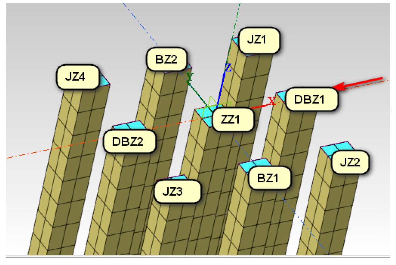
A large number of studies show that in a pile group foundation, each foundation pile bears different loads transmitted from the bearing platform plate, and the soil around the foundation piles at different positions also has different effects on the pile, making it difficult to compare and analyze them. In this section, the foundation pile ZZ1 at a specific location was selected for the analysis of the vertical bearing characteristics of the pile during vibration. To facilitate the analysis, the cumulative coefficient of the pile side friction resistance CCPF was introduced in this paper:

$$CCPF=\frac{{\sum }_{i=1}^n(N_{i+1}-N_i)}{P_0}\times 100\%$$

(17)

The pile was divided into n sections, where N_i+1 and N_i are the axial forces at sections i and i + 1 of the pile body, respectively, and P foundation represents the sum of the side friction resistance of the pile under an equivalent load Q. P₀ = Q − N_min, 9 pile was adopted in the model, where Q takes 1/9 of the load on the bearing cap, and N_min is the axial force at the bottom of the pile (considered as the resistance at the end of the pile).

The value of the CCPF reflects the distribution of soil friction along the side of the pile, and the change in the CCPF reflects the change in the side friction resistance. In liquefied sites, liquefaction of the soil layer under horizontal seismic forces will lead to a decrease in the shear strength of the soil, which will naturally reduce the friction on the side of the pile provided. The axial force of the pile body will inevitably change with the change in the pile side friction. Such a change in trend and law can be reflected in the change in the cumulative coefficient of the pile side friction.

6.1. Model Validation

Many studies suggest that when the pore pressure ratio reaches around 0.8, the soil will begin to liquefy, and when the pore pressure ratio reaches 1.0, the soil will be completely liquefied (having lost its shear resistance):

$$\mathrm{pore} \mathrm{pressure} \mathrm{ratio}=∆P/{\sigma }_{zz}$$

(18)

where $∆P$ is the difference between the measured pore water pressure value and the initial value, also known as the excess pore water pressure, and ${\sigma }_{zz}$ is the effective stress of the soil in the direction of gravity at the measurement time.

The pore pressure ratio–time history curves of the shaking table model test and numerical model calculation at different depths of measurement points under horizontal seismic action were drawn. The representative values of the measurement points 5 cm, 30 cm, and 50 cm below the soil layer were selected. Figure 13 shows the results of the shaking table test, and the pore pressure ratio curve of the natural site without pile foundation reinforcement. The abscissa axis is the vibration time (s), and the ordinate is the pore pressure ratio. From the curve trend, it can be seen that the pore pressure ratio of the surface soil reached 0.8 around 14 s, indicating that the soil began to liquefy. As the depth increased, the liquefaction lagged behind relatively. The liquefaction of the surface soil was the most severe, and the liquefaction situation gradually decreased towards the deeper layers. The maximum pore pressure ratio reached around 1.3. The overall soil layer was completely liquefied in about 18 s, with the peak pore pressure being the highest compared to the surface layer (5 cm), followed by the middle layer (30 cm) and the bottom layer (50 cm).

The numerical simulation results (Figure 14) were basically consistent with the experimental results. The surface soil began to liquefy around 13 s, and the overall soil layer entered a fully liquefied state around 18 s. The peak pore pressure ratio of the soil at 20 s indicated that the shear resistance of the surface layer of the foundation almost disappeared, and the peak pore pressure ratio reached around 1.35. After the vibration, the pore pressure of the surface soil dissipated the fastest, followed by the middle layer, with the dissipation being the slowest at the bottom layer. However, there was no obvious dissipation phenomenon in the data curve obtained in the shaking table test, mainly due to the unsatisfactory drainage conditions set in the experiment and the measurement error of the sensor. The numerical calculation results were relatively close to the experimental results, indicating that the selection of numerical analysis models and related parameters was reasonable, in terms of dynamic calculation.

6.2. CCPF Distribution Law and Characteristics of the Single-Pile System along the Pile Body

Firstly, a single-pile system was selected as the research object. By analyzing the distribution rule and characteristics of the CCPF along the pile body, the change in the vertical bearing capacity of the single pile during an earthquake was further analyzed to verify whether the CCPF can reflect the common action mechanism of the pile and soil comprehensively and reasonably. The vibration time points were 0 s, 15 s, 25 s, and 35 s. The pile stress was recorded every 5 cm along the pile body. According to the stress, the axial force can be obtained, and then the side friction resistance of each section of soil around the pile can be obtained. In the laboratory test, a 750 N load was applied before the vibration of the pile group foundation composed of 9 piles. Therefore, 1/9 of the pile group, i.e., 83.33 N, was applied to the single pile. From the model calculation, the stress of the pile body was obtained directly; then, the curve of the CCPF along the pile body at different specific moments of the earthquake action was obtained via further calculation (see Figure 15). The corresponding change values are shown in

Table 5. The change values of the CCPF at different positions of the pile during shaking.

Shaking Time (s)	Longitudinal Depth of Pile (cm)
	0	−5	−10	−15	−20	−25	−30	−35	−40	−45	−50	−55	−60
0	0	5	11	17	28	39	49	61	70	79	85	93	100
15	0	0	1	6	12	18	27	36	54	70	81	91	98
25	0	0	0	1	2	4	9	16	28	37	59	75	90
35	0	0	0	0	1	2	3	5	10	21	32	51	75

. In addition, for the purpose of analysis, static load tests were carried out on the pile–soil system at different vibration times, and the corresponding Q–S curve was obtained, as shown in Figure 16. The relevant values are shown in

Table 6. Relationship between the vertical force and settlement of the single pile at different specific shaking times.

Shaking Time (s)	Vertical Force (N)
	80	100	120	140	160	180	200	220	240	260	280	300
0	0	−0.7	−1.4	−1.9	−2.6	−3.9	−6.2	−8.4	−12.3	−22.1	−37	−48.2
15	−1.3	−3.8	−6.2	−9.1	−12.7	−17.8	−21.9	−35	−46	----	----	----
25	−2.2	−6.7	−11.4	−16.3	−24.1	−35	−47	----	----	----	----	----
35	−3.5	−10.4	−18.1	−29.8	−39.1	----	----	----	----	----	----	----

.

As can be seen in Figure 8, with the duration of vibration, the CCPF increased rapidly at the same vibration time within the range of 0~−40 cm along the pile, but, with a longer vibration time, the CCPF of the same pile decreased significantly. In the range of −40~−60, at 0 s and 15 s, the CCPF maintained the same growth rate as at 0~−40 cm, but, at 25 s and 35 s, the growth rate of the CCPF significantly slowed down. Moreover, it can be seen that the CCPF at the bottom of the pile was reduced from 100% to 74% at 0 s. Based on the analysis of Figure 9, it can be seen from the Q–S curve that the curve steepened, and the ultimate bearing capacity gradually decreased with the duration of the vibration. The ultimate bearing capacity of the single pile was about 220 N at 0 s, 150 N at 15 s, and 120 N at 25 s. The curve dropped sharply at 35 s, and the bearing capacity decreased. Combined with the CCPF and Q–S curves, it can be seen that, when the vibration time was short (within 15 s), the soil was not liquefied, and CCPF = 1 at the bottom of the pile indicates that the actual load acting on the top of the pile in a short time was equal to the applied load. As the vibration time increased continuously, the soil around the pile began to liquefy from top to bottom. The liquefied soil layer reduced the friction resistance on the side of the pile, but the actual load acting on the top of the pile was less than the load applied on the top of the pile. Thus, the phenomenon that the CCPF at the bottom of pile was less than 1 at 25 s and 35 s appeared.

The above analysis shows that the CCPF can intuitively reflect the distribution rule of the accumulated pile side friction resistance along a pile body during an earthquake. By comparing the value of the CCPF at the bottom of pile with the value of 1, the change in the actual load on the top of the pile during vibration can be clearly analyzed.

6.3. Distribution Regularity and Characteristics of CCPF along the Pile Body of a Pile Group System

The same analysis was carried out for piles in a pile group foundation, by means of the CCPF. Figure 10 shows the CCPF curve of the ZZ1 pile at different times of seismic action, when the spacing between piles was 3D, 3.5D, 4D, 5D, and 6D. The relationships between the vertical force and settlement of the 3D, 3.5D, 4D, 5D, and 6D working conditions at different specific shaking times are shown in

Table 7. The CCPF value of ZZ1 during shaking at specific shaking times under the 3D working condition.

Shaking Time (s)	Longitudinal Depth of Pile (cm)
	0	−5	−10	−15	−20	−25	−30	−35	−40	−45	−50	−55	−60
0	0	5	8	13	18	24	29	35	41	52	60	67	75
15	0	4	6	9	13	18	23	30	40	51	63	75	86
25	0	2	4	5	7	10	14	20	34	52	71	85	100
35	0	0	1	3	6	9	10	14	26	40	62	86	118

,

Table 8. The CCPF value of ZZ1 during shaking at specific shaking times under the 3.5D working condition.

Shaking Time (s)	Longitudinal Depth of Pile (cm)
	0	−5	−10	−15	−20	−25	−30	−35	−40	−45	−50	−55	−60
0	0	4	7	12	16	23	29	33	38	45	54	62	70
15	0	3	5	9	12	17	21	26	32	40	52	64	81
25	0	1	3	6	9	10	13	18	27	39	58	79	94
35	0	0	1	2	4	7	10	15	24	43	61	85	111

,

Table 9. The CCPF value of ZZ1 during shaking at specific shaking times under the 4D working condition.

Shaking Time (s)	Longitudinal Depth of Pile (cm)
	0	−5	−10	−15	−20	−25	−30	−35	−40	−45	−50	−55	−60
0	0	3	6	10	15	20	26	31	38	43	51	58	65
15	0	1	2	4	8	12	17	24	31	42	53	64	78
25	0	0	1	3	5	7	10	14	18	25	43	64	89
35	0	0	0	2	3	5	7	9	14	20	34	61	94

,

Table 10. The CCPF value of ZZ1 during shaking at specific shaking times under the 5D working condition.

Shaking Time (s)	Longitudinal Depth of Pile (cm)
	0	−5	−10	−15	−20	−25	−30	−35	−40	−45	−50	−55	−60
0	0	2	5	10	15	20	26	31	38	43	50	57	63
15	0	1	2	4	8	12	17	24	31	42	53	64	79
25	0	0	1	2	5	7	10	15	20	29	42	63	90
35	0	0	0	1	3	7	11	15	18	24	33	58	92

and

Table 11. The CCPF value of ZZ1 during shaking at specific shaking times under the 6D working condition.

Shaking Time (s)	Longitudinal Depth of Pile (cm)
	0	−5	−10	−15	−20	−25	−30	−35	−40	−45	−50	−55	−60
0	0	2	4	9	14	19	25	30	37	44	51	57	62
15	0	1	2	4	8	11	15	22	29	40	50	64	75
25	0	0	1	2	5	7	12	15	20	29	42	63	86
35	0	0	0	1	3	7	10	16	19	25	35	59	92

.

By analyzing the 3D working condition, the CCPF value at the same position of the pile body decreased gradually with the extension of the vibration time in the range of 0 to −50 cm, while it increased gradually in the range of −50 cm to −60 cm. The distribution curve of the CCPF at each moment intersected at −40~50 cm of the pile body, and the maximum value of the CCPF occurred at the bottom of the pile at each moment of vibration, from 0.75 at 0 s to 1.28 at 35 s; the maximum CCPF at 0 s and 15 s was less than 1. In line with previous research [16,21], no liquefaction occurred in the soil around the pile before 20 s of vibration, which indicates that the actual load on the top of the ZZ1 pile was less than the average of the total load. After 20 s of vibration, the soil began to liquefy, being approximately equal to 1 at 25 s, indicating that the load on the top of the pile was approximately equal to the average of the total load. The value was greater than 1 at 35 s, which indicates that, with the continuous liquefaction of the soil from top to bottom, the bearing load of the soil between piles decreased gradually, due to the pile group effect, and the bearing load of each foundation pile increased accordingly, which indicates that the bearing load on the top of the ZZ1 pile was greater than the average of the total load (Figure 17).

Under the 3.5D working condition, the change in curves of the CCPF values at different vibration times were similar. According to the analysis of the 3D working condition, the load on the top of the pile was only greater than the average value when the vibration lasted 35 s, while the load at the other times was less than the average value. From the CCPF distribution curve, it can be seen that the intersection point moved down a little along the pile body, compared with the 3D condition, around −50 cm.

The distribution characteristics of the CCPF curves under the 4D, 5D, and 6D conditions were the same. At each vibration moment, the value of the CCPF at the bottom of the pile was less than 1, which means that the load at the top of the pile was less than the average value of the total load at each time. The steepness of the CCPF curve reflects the change degree of the friction resistance along the side of the pile body at each moment of vibration. Because the actual load on the top of the pile varied with the liquefaction degree at each moment of vibration, the CCPF value could not reflect the friction resistance on the side of the pile at each time, and there was no comparability. The intersection points were all concentrated at −50 cm, which continued to decline, compared with the 3.5D condition. The variation curve of the CCPF at the bottom of the middle pile (ZZ1) in the pile group foundation with the vibration time is shown in Figure 18 (for the relevant data, see

Table 12. The CCPF at the bottom of ZZ1 during shaking, under the different working conditions.

Different Times	Pile Spacing (D)
	3	3.5	4	5	6
0 s	75	70	65	63	64
15 s	86	81	78	79	78.5
25 s	100	94	89	90	87.8
35 s	118	111	94	92	91.5

).

Figure 18 shows that, under certain pile spacings, the value of the CCPF gradually increased with the duration of the vibration, which indicates that the actual load on the top of the ZZ1 pile increased with the increase in vibration time. At the same vibration time, the CCPF value decreased with the increase in pile spacing, and the actual load on the top of the pile decreased with the increase in pile spacing.

7. Conclusions and Suggestions

7.1. Conclusions

In this study, the cumulative coefficient of the pile side friction resistance CCPF was introduced. According to the distribution of the foundation piles (middle piles) in a single pile and in pile groups with different pile spacings along the CCPF of the pile body, the following can be concluded:

The CCPF intuitively reflected the distribution pattern of the accumulated frictional resistance along the pile body during the vibration process. When the spacing between piles was constant, the value of the CCPF gradually increased with the vibration time. The actual load on the top of the pile increased with the increase in vibration time.

At the same vibration time, the CCPF value decreased with the increase in pile spacing, and the actual load on the top of the pile decreased with the increase in pile spacing.

When the value of the CCPF at the bottom of the pile was equal to 1, the actual load on the top of the pile was equal to the average value of the total load. When the CCPF at the bottom of the pile was less than 1, the load on the top of the pile was less than the average value of the total load. When the CCPF at the bottom of the pile was greater than 1, the load on the top of the pile was greater than the average of the total load.

7.2. Suggestions

(1)

For specific reasons, using a pile group system, this work studied the variation characteristics of the lateral friction resistance of the central pile during vibration. However, further research is needed on the variation in the lateral friction resistance of the edge and corner piles during the vibration process.

(2)

The vibration parameters (fundamental frequency, amplitude, duration, etc.) are the main influencing factors regarding the dynamic characteristics of the soil. In the future, we will further study the dynamic characteristics of soil with different vibration parameters.