Railway Freight Demand Forecasting Based on Multiple Factors: Grey Relational Analysis and Deep Autoencoder Neural Networks

Abstract

The construction of high-speed rail lines in China has drastically improved the freight capacity of conventional railways. However, due to recent national energy policy adjustments, rail freight volumes, consisting mostly of coal, ore, and other minerals, have declined. As a result, the corresponding changes in the supply and demand of goods and transportation have led to a gradual transformation of the railway freight market from a seller’s market to a buyer’s market. It is important to carry out a systematic analysis and a precise forecast of the demand for rail freight transport. However, traditional time series forecasting models often lack precision during drastic fluctuations in demand, while deep learning-based forecasting models may lack interpretability. This study combines grey relational analysis (GRA) and deep neural networks (DNN) to offer a more interpretable approach to predicting rail freight demand. GRA is used to obtain explanatory variables associated with railway freight demand, which improves the intelligibility of the DNN prediction. However, the high-dimension predictor variable can make training on DNN challenging. Inspired by deep autoencoders (DAE), we add a layer of an encoder to the GRA-DNN model to compress and aggregate the high-dimension input. Case studies conducted on Chinese railway freight from 2000 to 2018 show that the proven GRA-DAE-NN model is precise and easy to interpret. Comparative experiments with conventional prediction models ARIMA, SVR, FC-LSTM, DNN, FNN, and GRNN further validate the performance of the GRA-DAE-NN model. The prediction accuracy of the GRA-DAE-NN model is 97.79%, higher than that of other models. Among the main explanatory variables, coal, oil, grain production, railway locomotives, and vehicles have a significant impact on the railway freight demand trend. The ablation experiment verified that GRA has a significant effect on the selection of explanatory variables and on improving the accuracy of predictions. The method proposed in this study not only accurately predicts railway freight demand but also helps railway transportation companies to better understand the key factors influencing demand changes.

1. Introduction

Rail freight transportation is an environmentally friendly, economical, and sustainable method of transportation that is critical for efficient and cost-effective long-haul freight and freight transportation. It is particularly important for the movement of bulk materials, such as coal, petroleum, and grain, as well as heavy machinery and other large items that cannot be easily transported by other modes of transportation. Railway freight transportation is also a key component of global trade, connecting producers and consumers across different regions and countries. Therefore, the reliability of railway freight transportation plays a crucial role in ensuring the stable operation of the global supply chain, driving economic growth, enhancing social connectivity, and achieving sustainable development. An accurate understanding of the demand in the railway freight market is a prerequisite for improving service reliability. Accurate forecasting of railway freight demand helps railway companies estimate cargo volumes, allowing them to plan resources, improve operations, and provide customers with more stable and reliable services. In recent years, China has constructed the longest and most complex high-speed railway network in operation today [1]. The major railway lines in China have achieved the separation of passenger and freight transport, and the freight transport capacity has been considerably enhanced [2]. However, with the adjustment of the national energy policy, the main freight transportation of railways, such as coal and ore, has decreased, which has forced railway freight enterprises to look for other sources of goods [3]. The market pattern of railway freight transportation is gradually shifting from a seller’s market to a buyer’s market, and railway freight transportation enterprises are also shifting from simply meeting the demand for transportation volume to meeting the multiple demands of shippers. Adapting to changes in the market, understanding shipper demand, and conducting systematic analyses and forecasts of the rail freight market are of major importance.

Researchers have done much work on prediction, and the theoretical system is quite mature. The predictive approach could be divided into two types, qualitative analysis and quantitative analysis. The first approach mainly utilizes specialist experience to analyze the specific characteristics of freight transportation and accurately predict the freight volume by integrating various relevant influencing factors. This means that qualitative analysis is often limited by subjective experience. The second approach focuses on exploiting the relationships among historical data, which are then used to build the prediction model. Predicting the change level of this statistical index in the next period through the development process and changing trends reflected by a certain statistical index arranged in a time series. Widely used methods include linear theory [4,5,6], intelligent fuzzy prediction [7,8], and non-linear system theory [9,10]. However, such methods are based on human experience and lack generality. Once the environment changes, precise predictions cannot be achieved.

To overcome the theoretical limitations of these methods, researchers focused on development in the artificial neural network (ANN) field, which simulates the structure of human brain neurons and their related mechanism of action, abstracts, and builds a relatively simple model [11]. ANN is a non-linear, adaptive treatment system with multiple treatment units. By constructing a hidden layer with several nodes between the input layer and the output layer of the network, the nodes relate to each other, and the output of each layer is the input of the lower layer to construct an interrelated neural network. However, with the deepening of the research, the disadvantages of the artificial neural network model, such as complicated steps, large amounts of computation, and complex algebraic functions, are obvious due to the need for artificial feature extraction. Deep learning differs from the shallow learning concept of artificial neural networks. By increasing the number of hidden layers, complex function problems can be addressed with fewer parameters, ensuring that the original information of the data remains unchanged despite changes in dimensions [12]. This simplifies the processing and implementation of the data. Deep learning models are widely used for predicting data patterns across multiple domains [13,14,15]. However, the black box (of every unexplored object) characteristic of deep neural networks (DNN) results in poor interpretability of prediction results. Decision-makers can only know the future demand trends, but they do not know the reasons that affect demand change, cannot evaluate their reliability, and are not able to accurately formulate response strategies.

Combining DNN with other factor analysis methods to explore data patterns and features before modeling and then proposing explanatory variables for the model is an effective method to improve the interpretability of the model. In the quantitative methods of factor analysis, most of them adopt mathematical statistics analysis methods such as regression analysis, variance analysis [16], etc. However, they require samples to have good distribution laws such as linear, exponential, or logarithmic, but there are disadvantages, such as large calculation workload. Based on multiple data sources, the researchers used the newspaper vendor model [17] and the decision tree method [18] to predict the flow of bus passengers. These methods offer advantages in terms of prediction accuracy and stability. They also provide stronger explanatory power in determining the relative contribution and priority of influencing factors to the prediction. In addition to identifying the contributions of influencing factors to the forecasting model, we also need a method to select the best explanatory variables from numerous influencing factors. Grey relational analysis (GRA) is a method of measuring the degree of correlation between factors based on the degree of similarity or dissimilarity in their development trends [19]. Grey correlation analysis is also used to predict data patterns influenced by multiple factors [20,21,22]. However, the method of using GRA to select many explanatory variables and then applying a deep learning model for data feature learning to achieve railway freight volume prediction has limitations. The inclusion of many explanatory variables increases the dimension of the input data. This implies the need to form more pattern parameters, thus increasing the complexity of the algorithm. Increased workload and the difficulty of learning the characteristics of high-dimensional data present challenges, making it difficult to apply this method in real-life scenarios.

Automatic Encoders (AE) can automatically learn and retrieve characteristics from raw data without manual design and selection [23]. Using the structure of an encoder and a decoder, an autoencoder can extract and reconstruct key features from input data. It also compresses high-dimensional data through encoding before training, reducing the number of parameters to be trained. This process enhances the learning efficiency of deep neural networks (DNNs) and improves the model performance. [24]. Compared with traditional automatic encoders, the advantages of deep automatic encoders (DAE) [25] are:

• Stronger representation learning ability: Deep automatic encoders can adaptively learn high-level feature representations. This makes it possible to distinguish the differences between the categories and to improve the accuracy of the model;
• Non-linear modeling capability: Deep automatic encoders adopt a multilayered non-linear transformation, which can better approximate the non-linear function, thus improving the performance of the model;
• Stronger generalization ability: Deep automatic encoders can map raw data to higher-level, more abstract representation spaces, improving the model’s generalizability.

To adapt to different conditions and meet various task requirements, researchers have adjusted and improved the automatic encoders, including sparse automatic encoders [26,27], noise reduction automatic encoders [28], edge noise reduction automatic encoders [29], stack noise reduction automatic encoders [30], and so on. In recent years, automatic encoders have been used for multi-dimensional feature extraction for defect detection [31], medical image clustering [32], and image segmentation [33], among others. However, these tasks about clustering and correlation are all based on the unsupervised learning DAE model. DAE cannot be directly used for regression or classification works in freight demand prediction. Research [34] established a semi-supervised learning DAE model considering label constraints for classification tasks. Based on this, we improved the DAE in the way of supervised learning and proposed a railway freight demand forecasting method with strong capabilities for representation, generalization, and non-linear modeling.

Therefore, we put forward a supervised learning GRA-DAE-NN prediction model. It can select key explanatory variables and indicators with a high correlation to railway freight demand based on GRA. Unlike existing research, we believe that the prediction of railway freight demand is influenced by railway transportation capacity, supply market demand, and other forms of competition, considering factors such as demand, competitors, and supply, respectively. Obtaining the explanatory variables for demand forecasting and using them as inputs, the DAE-NN model is then used to predict railway freight demand. The GRA-DAE-NN model has a strong capacity for non-linear modeling and representation, generalizability, and good interpretability.

The main contributions of this article are as follows: (1) We propose a more interpretable method for predicting railway freight demand by combining grey relational analysis (GRA) with a DNN model. GRA is used to obtain explanatory variables related to the prediction of railway freight demand, while the DNN model is used to learn the feature correlation between these variables and railway freight demand, enabling the prediction of railway freight demand. Decision makers can better understand the reasons for the changes in demand trends by observing the variations in the explanatory variables, thereby improving the accuracy of response strategies such as capacity resource allocation and matching freight sources. (2) To further modify the model, we introduce the deep autoencoder (DAE) and improve the above-mentioned model in the GRA-DAE-NN model. This model takes advantage of the DAE to compress the high-dimensional explanatory variables and adaptively learn data features. It addresses challenges faced by the GRA-DNN model, such as difficulties in extracting high-dimensional data features, complex modeling stages, high computational complexity, and resource-intensive calculations. Furthermore, the design of the decoder structure retains the intelligibility of the original explanatory variables for rail freight demand. (3) We conducted testing using real cases and compared the proposed prediction method with mainstream forecasting methods in the same case. The findings validated the effectiveness of the proposed forecasting method.

The other parts of this article are organized as follows. In the second part, we present the proposed GRA-DAE-NN model and its method for railway freight demand prediction. In the third part, we conduct a case study to experimentally test the model’s performance using real data, comparing it with current mainstream prediction models. The fourth part includes research conclusions and limitations of the model.

2. Methodology

2.1. The Problem Formulation

Accurately predicting freight demand is of great significance in the current railway transportation industry for optimizing resource allocation, improving service reliability, and promoting the sustainable development of the railway transport sector. The problem addressed in this study is to propose a comprehensive and interpretable method for predicting railway freight demand using multiple data sources, aiming to meet the needs of railway transport enterprises for accurate prediction and resource planning. The problem of forecasting rail freight demand can be formulated as a problem of non-linear modeling and regression, which can be expressed as follows:

$$X_i=\left(x_{i1},x_{i2},x_{i3}\cdots x_{in}\right)\stackrel{F(•)}{\to }{Y}_i$$

(1)

where $Y_i$ represents the target of railway freight demand prediction, $F(•)$ is a hidden function with railway freight-related influencing factors as explanatory variables, and $X_i$ represents explanatory variables. $X_i$ and $Y_i$ are time series data.

This study combines grey relational analysis (GRA), deep autoencoder (DAE), and neural networks (NN). GRA is used for the selection of the explanatory variable set $X_i$. DAE-NN encodes and aggregates the high-dimensional $X_i$, learns the hidden data features of $X_i$, and uses them to predict railway freight demand. It is worth noting that $Y_i$ can represent either the overall demand for railway freight or the transportation demand for a specific category of goods. Depending on the specific prediction target, the candidate set $X_i$ and the selected set of explanatory variables may vary.

2.2. The GRA-DAE-NN Model

The model is divided into two parts: GRA is used to obtain the explanatory variables for railway freight demand prediction from a large set of factors related to railway freight; DAE-NN is to learn the feature correlations between the explanatory variables and railway freight demand, thus achieving the prediction of railway freight demand trends.

In quantitative methods of system analysis, regression analysis, variance analysis, and other mathematical methods of statistical analysis are routinely used. However, these methods have certain drawbacks, such as the requirement for large data volumes, adherence to distribution rules such as linearity, exponentiation, or logarithm of samples, and substantial computational workload. To address these limitations, Professor Deng Yulong proposed the grey system theory. Grey correlation analysis, a fundamental component of grey system theory, measures the correlation among factors based on the similarity or difference degree of each factor sequence at any given time or the development trend of different objects. It applies geometric processing to the data sequence of certain factors and determines the correlation concerning the magnitude of synchronous changes between factors. If the development trend among factors is similar, indicating a high degree of synchronous change, then the correlation between them is considered high. Conversely, if the development trend differs, the correlation is considered low. This method is straightforward in principle, offering clear ordering, and does not impose specific requirements on the correlation between data distribution types and factor variables. Consequently, grey correlation analysis is frequently used for quantitative analysis of system development and change.

Traditional methods for qualitative analysis of the factors influencing the freight market are based on empirical experiences and lack theoretical foundations. In addition, DNN-based prediction methods for time series data suffer from a lack of interpretability. To address these challenges, this paper adopts the grey relational analysis (GRA) method, building upon qualitative analysis. The factors exhibiting the highest correlation with the railway freight market are selected as explanatory variables for predicting freight volume in the railway freight market. This approach aims to explain the changes in railway freight demand.

The grey correlation analysis steps are as follows:

• Step 1. Determine the characteristic sequence $X_0=\left(x_{01},x_{02},\cdots ,x_{0j},\cdots ,x_{0n}\right)$;
• Step 2. Determine the correlation factor sequence $X_i=\left(x_{i1},x_{i2},\cdots ,x_{ij},\cdots ,x_{in}\right)$;
• Step 3. The reference and comparison sequences are normalized. The dimensionless characteristic sequence $Y_0=\left(y_{01},y_{02},\cdots ,y_{0j},\cdots ,y_{0n}\right)$ and the dimensionless correlation factor $Y_i=\left(y_{i1},y_{i2},\cdots ,y_{ij},\cdots ,y_{in}\right)$, $i=1,2,\cdots ,m$;
• Step 4. Find the correlation coefficient between the reference sequence and comparison sequence ${\gamma }_{0i}$.

$${\gamma }_{0i}\left(j\right)=\frac{\underset{i}{\min }\left[\underset{j}{\min }\left(|y_{0j}-y_{ij}|\right)\right]+\xi \underset{i}{\max }\left[\underset{j}{\max }\left(|y_{0j}-y_{ij}|\right)\right]}{|y_{0j}-y_{ij}|+\xi \underset{i}{\max }\left[\underset{j}{\max }\left(|y_{0j}-y_{ij}|\right)\right]},\begin{array}{l}i=1,2,\cdots ,m\\ j=1,2,\cdots ,n\end{array}$$

(2)

$${\gamma }_{0i}=\frac{1}{N}{\displaystyle \sum _{j=1}^n{\gamma }_{0j}}$$

(3)

where ${\gamma }_{0i}\in \left(0,1\right]$, the greater the ${\gamma }_{0i}$, the closer the relationship between the sequences, and the rank of correlation. Order the factor $i$, $i=1,2,\cdots ,m$ according to the calculated correlation degree ${\gamma }_{0i}$. The relative order of the degree of correlation of each factor to the characteristic of the system sequence, namely the correlation order, can be obtained.

GRA is used to obtain explanatory variables related to the prediction of railway freight demand. Decision-makers can better understand the reasons for shifts in demand patterns by observing the variations in the explanatory variables, thereby improving the accuracy of response strategies.

The deep autoencoder (DAE) is a kind of deep learning model with improved efficiency of feature extraction, while its production and application no longer need to manually extract the data characteristics. The basic idea is through greed and systemic training, step by step, unsupervised non-linear network extraction parameters optimization of multi-layer hierarchical characteristics of the input data, and distributed features of the original data of the deep learning neural network structure.

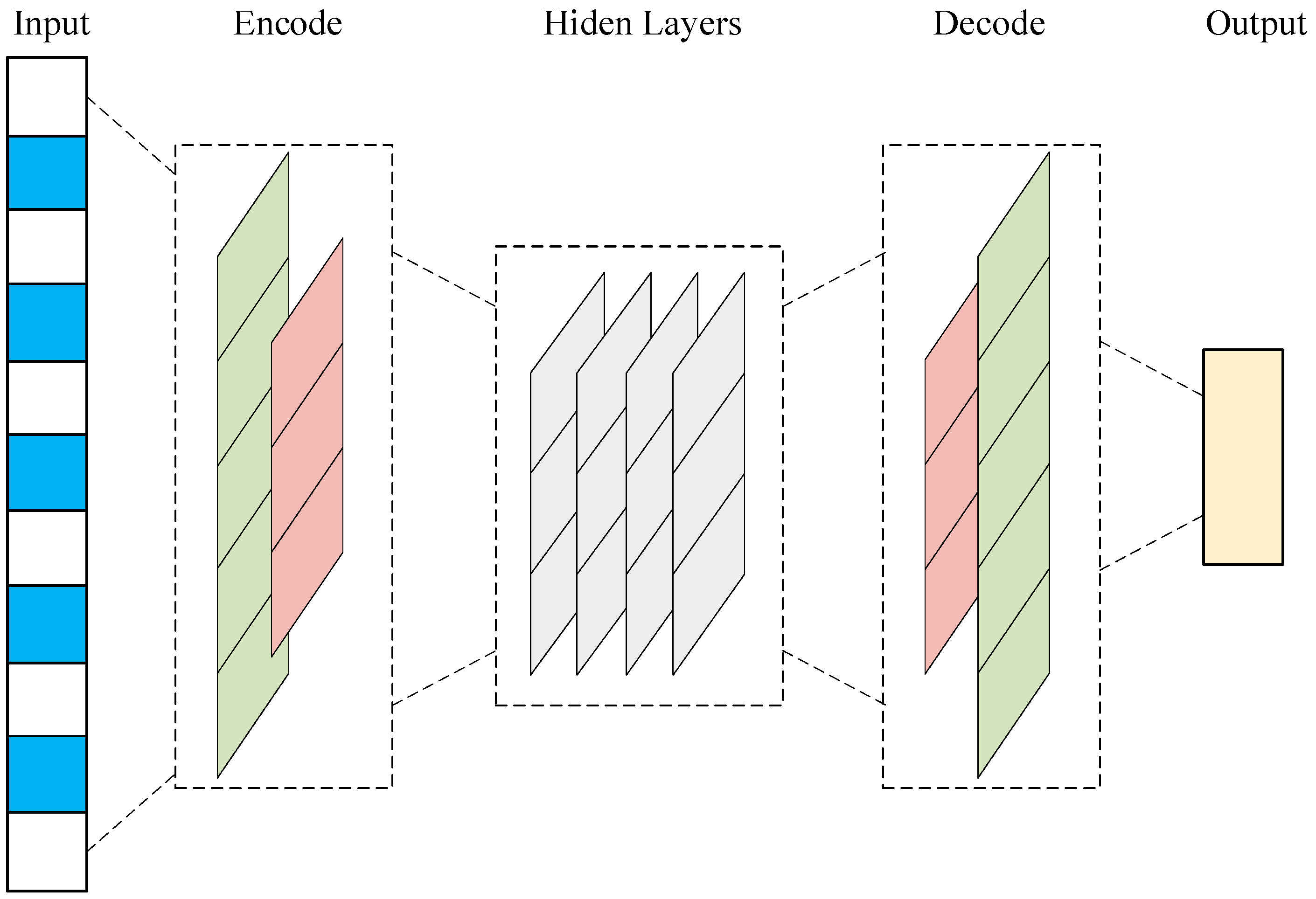
By increasing the number of hidden layers, complex function problems can be obtained by setting fewer parameters so that the original information of the data cannot be changed while the dimension changes and data processing and application can be simplified. Figure 1 presents a schematic diagram of the deep learning model structure.

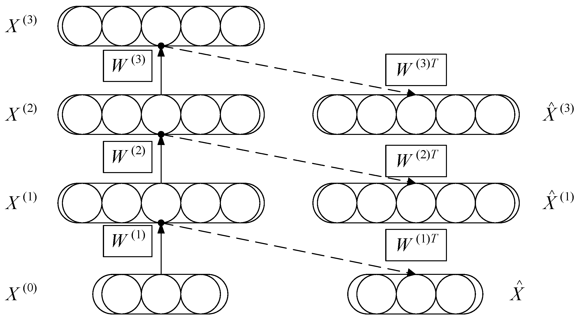
DEA consists of hidden layers, an encoder, and a decoder. The encoder encodes the data between the input layer and the hidden layer and then decodes the data between the hidden layer and the input layer. The reconstruction of input data is carried out by the process of decoding multi-dimensional data. By adding fitting layers, the prediction of railway freight demand can be achieved from multiple explanatory variables. The structure of the improved DAE-NN model is shown in Figure 2.

a.

Encoder

Encoder is the mapping from the input layer data $x$ to the node of the hidden layer $h$, and the mapping relation is as follows (4).

$$h=f\left(x\right)=S_f\left(W+b_n\right)$$

(4)

where $S_f$ is the non-linear activation function of the encoder, using $sigmoid$ function as shown in Formula (5). $W$ is weight matrix, denoted as $w^T$.

$$sigmoid\left(z\right)=\frac{1}{1+z^{-1}}$$

(5)

b.

Decoder

The decoder maps the hidden layer data back to refactoring $y$. The mapping relation is as follows (6):

$$y=g\left(h\right)=S_g\left(W^{\prime }h+b_y\right)$$

(6)

where $S_g$ is the non-linear activation function of the encoder, using $sigmoid$ function.

c.

Training process

The process of training DAE is to find the minimum reconstruction error of the parameter $\theta =\left\{W,b_y,b_h\right\}$ that is on the training sample set D, and the reconstruction error is expressed as follows:

$$J_{AE}={\displaystyle \sum _{x\in D}L\left(x,g\left(f\left(x\right)\right)\right)}$$

(7)

where L is the reconstruction error function, generally the square error function or the cross-entropy loss function. When $S_g$ is the identity function, L is a mean absolute difference, shown as follows (8).

$$L\left(x,y\right)={\Vert x-y\Vert }^2$$

(8)

when $S_g$ is $sigmoid$ function, L is cross-entropy loss function, as follows (9).

$$L\left(x,y\right)=-{\displaystyle \sum _{i=1}^{d_x}{x}_i}\log y_i+\left(1-x_i\right) \log \left(1-y_i\right)$$

(9)

Compared with the traditional DNN model (Figure 1), the DAE-NN model (Figure 2) reduces the dimensionality of the original input by compressing the high-dimensional explanatory variables obtained from GRA. This eliminates the significant workload of manually extracting data features and improves the efficiency of feature extraction. Furthermore, the design of the decoder structure preserves the interpretability of the original explanatory variables for railway freight demand.

2.3. Prediction Method Based on GRA-DAE-NN

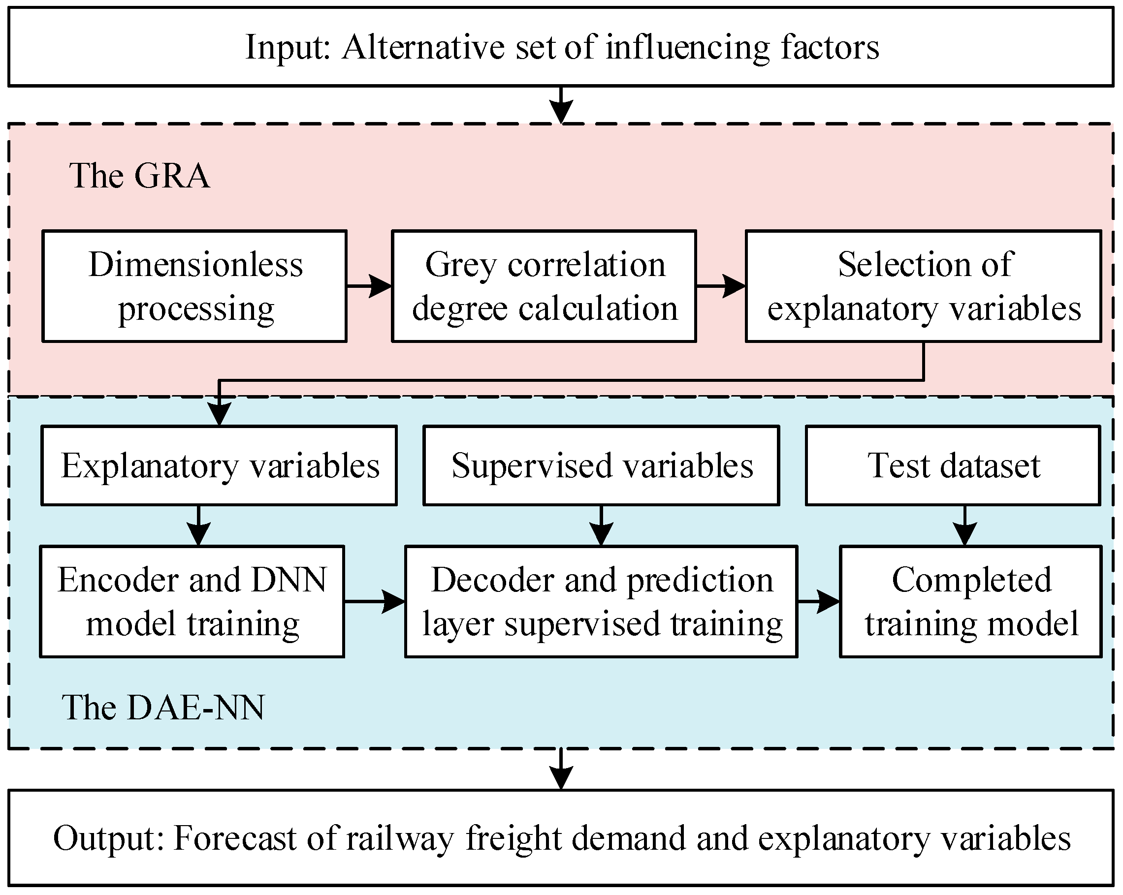
The process of predicting railway freight demand based on the GRA-DAE-NN model is shown in Figure 3.

Constructing an alternative set of influencing factors is based on the prediction target of railway freight demand, including demand feature time series vectors and related factor matrices. Once the feature sequence and the associated factor sequence have been determined, the grey correlation degree is calculated following the steps below:

Non-dimensionalization processing:

Due to the diverse economic significance, dimensions, and representation forms of indicator data, there is a lack of comparability. Therefore, a standard 0–1 transformation is used to non-dimensionalize the data and eliminate the influence of dimensional units.

Forward indicators:

$$y_{ij}=\frac{x_{ij}-\underset{i}{\min } x_{ij}}{\underset{i}{\max } x_{ij}-\underset{i}{\min } x_{ij}}, 0\le i\le m, 1\le j\le n$$

(10)

Reverse indicators:

$$y_{ij}=\frac{\underset{i}{\max } x_{ij}-x_{ij}}{\underset{i}{\max } x_{ij}-\underset{i}{\min } x_{ij}}, 0\le i\le m, 1\le j\le n$$

(11)

After dimensionless processing, the indicator values are all in the range [0,1]. This article combines all indicators in references [35,36,37,38] to construct an alternative set of influencing factors for railway freight demand prediction. We have divided them into three aspects for factor selection: macroeconomics, related industry output, and competitive environment. Among the competitive factors, highways, waterways, and civil aviation form a competitive relationship with railway freight. The smaller the competitive environmental indicators, the higher the demand for railway freight. Therefore, the competitive environment indicator is a reverse indicator, while all other indicators are positive.

Calculate the grey correlation coefficient:

This involves calculating the correlation coefficient between the supervised variable and the candidate set of influence factors using Formulas (2) and (3). Among them, $\xi \in \left[0,1\right]$ is the discrimination coefficient. Generally, when $\xi \le 0.5463$, it is easier to observe the change in correlation resolution. While the value $\xi =0.5$ in this article, the correlation coefficient is the degree of correlation between feature vectors and related factors in a time series with a lot of information and dispersion. Therefore, the mean value is calculated as the quantitative relation of the degree of overall correlation. When the correlation degree (${\gamma }_{0i}\in \left(0,1\right]$) between each index ($X_i$) and railway freight volume ($Y_0$) is closer to 1, it indicates that this factor has a greater influence on railway freight volume.

The main process of constructing the railway freight market forecasting model based on DAE-NN is as follows:

DAE-NN framework construction:

Based on the structure of the prototype DAE, the basic framework of the DAE is constructed by increasing the number of hidden layers and neurons, adjusting the distribution of nodes in the hidden layers, and modifying the weight-sharing approach. In this study, a multi-layer cyclic iteration approach is applied to select the number of hidden layers ranging from 1 to 6 and the number of nodes ranging from 1 to 100, generating multiple iterations. Finally, the DAE network with three hidden layers and a small training error is chosen.

Pre-training of DAE-NN model:

The input layer is $X_i=(x_1,x_2,\cdots ,x_n)$. Where n is the factor affecting railway freight volume, the explanatory variables affecting the railway freight market demand (by GRA), and the railway freight volume reflecting the demand of the railway freight market are selected as the input data of DAE-NN, and the railway freight demand volume is taken as the output to construct the deep autoencoder network model.

To avoid neuron output saturation caused by overlarge inputs and accelerate the convergence of the training network, the model input index was standardized. The maximum normalization was adopted here, and the calculation formula is:

$$x_i^{\prime }=x_i/x_{\max }$$

(12)

where $x_i^{\prime }$ is the normalized index and $x_i$ is the original index value; $x_{\max }$ represents the maximum value of $x_i$.

The input layer and hidden layer of DAE are trained to make them all initialized, and then each hidden layer is trained as an automatic correlator by using the hierarchical greedy training algorithm to reconstruct the input data. The training process is shown in Figure 4. Through repeated training, its structural performance index is reduced, and its stability is strengthened.

Forecast of railway freight demand and model optimization:

The input layer, output layer, and all hidden layers of the DAE model of railway freight volume prediction were taken as a whole, and the supervised learning algorithm was used. The neural network algorithm was selected to further adjust it, and the ownership value and bias were optimized after multiple iterations.

The optimal trained and refined DAE-NN is used to forecast freight volumes. The prediction results are analyzed using the metrics of mean absolute error (MAE), mean absolute percentage error (MAPE), and root mean square error (RMSE). The formulas for calculating MAE, MAPE, and RMSE are as follows:

$$MAE=\frac{1}{N}{\displaystyle \sum _{n=1}^N\left|y_n-{\stackrel{⌢}{y}}_n\right|}$$

(13)

$$MAPE=\frac{1}{N}{\displaystyle \sum _{n=1}^N\left|\frac{y_n-{\stackrel{⌢}{y}}_n}{y_n}\right|}\times 100$$

(14)

$$RMSE=\sqrt{\frac{1}{N}{\displaystyle \sum _{n=1}^N{\left(y_n-{\stackrel{⌢}{y}}_n\right)}^2}}$$

(15)

In the above equation, $y_n$ is the predicted value, and ${\stackrel{⌢}{y}}_n$ is the true value, while $N$ represents the number of predicted values. MAE measures the average difference between predicted values and true values. MAPE measures the average percentage error. RMSE measures the magnitude of differences.

3. Case Study

This thesis validated the model using China railway freight market data from 2000 to 2018. The process involved first using GRA to select explanatory variables for predicting railway freight demand, followed by training the DAE-NN model for railway freight demand prediction. Additionally, we compared the GRA-DAE-NN model with seven baseline models. To validate the effectiveness of the model suggested in this study, we conducted experiments to assess its performance.

3.1. Data Source

The influencing factors related to railway freight demand forecasting, specifically macroeconomic conditions, relevant industry output, and competitive environment, were selected according to the method described in Section 2.3. The specific factors are shown in

Table 1. The influence factors of railway freight transportation market.

Classify		Influence Factor
Demand	Macroeconomy	Gross domestic product (GDP) ($X_1$)
		Total value of agricultural output ($X_2$)
		Total retail sales of consumer goods ($X_3$)
		Total volume of merchandise imports and exports ($X_4$)
	Related Industry Production	Coal production ($X_5$)
		Petroleum production ($X_6$)
		Steel production ($X_7$)
		Main non-ferrous metal production ($X_8$)
		Grain production ($X_9$)
		Express delivery volume of the year ($X_{10}$)
	Competitive Context	Freight traffic of highways ($X_{11}$)
		Freight traffic of shipping ($X_{12}$)
		Civil air cargo volume ($X_{13}$)
Supply		Investment in fixed assets in railway transportation ($X_{14}$)
		Length of railroad lines in service ($X_{15}$)
		National railway electrification mileage ($X_{16}$)
		Mileage of double track of national railways ($X_{17}$)
		National railway locomotive inventory ($X_{18}$)
		National railway freight wagon inventory ($X_{19}$)
		Number of railway employees ($X_{20}$)
		Wagon static load ($X_{21}$)
		Daily production of freight locomotives ($X_{22}$)

.

In terms of transport demand, changes in macroeconomic indicators such as GDP, agricultural output value, total retail sales of consumer goods, and total import and export trade of products will all impact the railway freight market. The points category according to railway goods traffic situation, railway freight volume is mainly dominated by coal, metal ore, steel and non-ferrous metal, petroleum, food, and other categories, so choosing coal production, petroleum production, steel production, mainly non-ferrous metals production, food production as rail freight market factors, which affect the demand side. In addition, with the rapid development of China’s e-commerce industry, the volume of express delivery has risen sharply, and the railway is also vigorously developing rail logistics. Therefore, express delivery volume is also considered a factor affecting the railway freight market. In terms of a competitive environment, highways, waterways, civil aviation, and rail transport replace each other and represent direct competitive relationships. Consequently, the freight volume of these three modes is chosen as the influencing factor.

In railway supply perspectives, fixed assets investment in the railway transport industry, railway operating mileage, national railway electrification mileage, double track mileage, freight cars, locomotive ownership, number of railway employees, a static load of freight cars, and daily output of locomotives are selected as the factors affecting the railway freight market.

The railway freight volume is chosen as the characteristic series reflecting the railway freight market. The railway freight volume of China from 2000 to 2018 is selected as the system characteristic series $X_0$, $X_1,X_2,\cdots ,X_{22}$ are, respectively, the relevant factors affecting railway freight volume. By consulting the website of the National Bureau of Statistics, China Traffic Statistical Yearbook, China Railway Yearbook, etc., 22 indicators influencing railway freight volume in 19 years from 2000 to 2018 were collected, shown in

Table 2. The demand-side influencing factors value of railway freight demand from 2000 to 2018.

Demand-Side Influencing		2000	2001	2002	2003	2004	2005	2006	2007	2008	2009
Macroeconomy	Gross domestic product (GDP) (billion CNY)	10,028.01	11,086.31	12,171.74	13,742.20	16,184.02	18,731.89	21,943.85	27,009.23	31,924.46	34,851.77
	Total value of agricultural output (billion CNY)	1387.36	1446.28	1493.15	1487.01	1813.84	1961.34	2152.23	2444.47	2767.99	2998.38
	Total retail sales of consumer goods (billion CNY)	3910.57	4305.54	4813.59	5251.63	5950.10	6835.26	7914.52	9357.16	11,483.01	13,304.82
	Total volume of merchandise imports and exports (billion DOLLAR)	474.29	644.37	814.45	984.52	1154.60	1421.91	1760.40	2173.83	2563.26	2207.54
Related Industry Production	Coal production (ten thousand tons)	138,418.50	147,152.70	155,040.00	183,489.90	212,261.10	236,514.60	252,855.10	269,164.30	280,200.00	297,300.00
	Petroleum production (ten thousand tons)	16,300.00	16,395.90	16,700.00	16,960.00	17,587.30	18,135.30	18,476.60	18,631.80	19,044.00	18,949.00
	Steel production (ten thousand tons)	13,146.00	16,067.61	19,251.59	24,108.01	31,975.72	37,771.14	46,893.36	56,560.87	60,460.29	69,405.40
	Main non-ferrous metal production (ten thousand tons)	783.81	883.71	1012.00	1228.06	1441.12	1635.00	1916.27	2379.15	2553.63	2648.54
	Grain production (ten thousand tons)	46,217.52	45,263.67	45,705.75	43,069.53	46,946.95	48,402.19	49,804.23	50,413.85	53,434.29	53,940.86
	Express delivery volume of the year (ten thousand piece)	11,031.40	12,652.70	14,036.20	17,237.80	19,772.00	22,880.30	26,988.04	120,189.56	151,329.30	185,785.81
Competitive Context	Freight traffic of highways (ten thousand tons)	1,038,813	1,056,312	1,116,324	1,159,957	1,244,990	1,341,778	1,466,347	1,639,432	1,916,759	2,127,834
	Freight traffic of shipping (ten thousand tons)	122,391	132,675	141,832	158,070	187,394	219,648	248,703	281,199	294,510	318,996
	Civil air cargo volume (ten thousand tons)	197	171	202	219	277	307	349	402	408	446
Demand-Side Influencing		2010		2011	2012	2013	2014	2015	2016	2017	2018
Macroeconomy	Gross domestic product (GDP) (billion CNY)	41,211.93		48,794.02	53,858	59,296.32	64,356.31	68,885.82	74,639.51	83,203.59	91,928.11
	Total value of agricultural output (billion CNY)	3590.907		4033.962	4484.572	4894.394	5185.112	5420.534	5565.989	5805.976	6145.26
	Total retail sales of consumer goods (billion CNY)	15,800.8		18,720.58	21,443.27	24,284.28	27,189.61	30,093.08	33,231.63	36,626.16	38,098.69
	Total volume of merchandise imports and exports (billion DOLLAR)	2972.761		3641.938	3866.8	4160.3	4303	3956.901	3684.914	4107.164	4622.415
Related Industry Production	Coal production (ten thousand tons)	342,844.7		351,600	394,512.8	397,432.2	387,391.9	374,654.2	339,437	352,356.2	368,121
	Petroleum production (ten thousand tons)	20,301.4		20,287.6	20,747.8	20,991.9	21,142.9	21,455.6	19,957.6	19,150.6	18,907.8
	Steel production (ten thousand tons)	80,276.58		88,619.57	95,577.83	108,200.54	112,513.12	103,468.41	104,813.45	104,642.05	110,551.65
	Main non-ferrous metal production (ten thousand tons)	3120.98		3628.94	3990.33	4412.13	4828.81	5155.82	5345.11	5498.31	5702.68
	Grain production (ten thousand tons)	55,911.31		58,849.33	61,222.62	63,048.2	63,964.83	66,060.27	66,043.51	66,160.72	65,789.22
	Express delivery volume of the year (ten thousand piece)	233,891.99		367,311.08	568,547.99	918,674.89	1,395,925.3	2,066,636.84	3,128,315.11	4,005,591.91	5,071,042.8
Competitive Context	Freight traffic of highways (ten thousand tons)	2,448,052		2,820,100	3,188,475	3,076,648	3,113,334	3,150,019	3,341,259	3,686,858	3,956,871
	Freight traffic of shipping (ten thousand tons)	378,949		425,968	458,705	559,785	598,283	613,567	638,238	667,846	702,684
	Civil air cargo volume (ten thousand tons)	563		557	545	561	594	629	668	706	739

and

Table 3. Supply-side influencing factors value of railway freight demand from 2000 to 2018.

Supply	2000	2001	2002	2003	2004	2005	2006	2007	2008	2009
Investment in fixed assets in railway transportation (billion CNY)	2622.18	3000.12	3548.88	4581.20	5902.80	7509.50	9336.90	11,746.40	14,873.80	19,392.00
Length of railroad lines in service (ten thousand km)	6.87	7.01	7.19	7.30	7.44	7.54	7.71	7.80	7.97	8.55
National railway electrification mileage (ten thousand km)	1.89	2.09	2.14	2.21	2.26	2.34	2.74	2.80	2.90	3.60
Mileage of double track of national railways (ten thousand km)	2.54	2.66	2.71	2.77	2.78	2.85	2.92	2.98	3.06	3.30
National railway locomotive inventory	14,472	14,955	15,159	15,456	16,066	16,547	16,904	17,311	17,336	17,825
National railway freight wagon inventory	439,943	453,620	459,017	510,327	526,894	541,824	564,899	577,521	591,793	601,412
Number of railway employees	1,871,000	1,789,271	1,758,421	1,727,735	1,698,667	1,665,588	1,652,720	1,741,029	1,732,909	1,850,147
Wagon static load (ton)	57.90	58.10	58.20	58.30	59.30	60.10	60.90	61.30	62.00	62.60
Daily production of freight locomotives (ten thousand ton-km)	99.40	99.90	102.20	105.80	108.70	110.60	114.30	120.40	123.60	128.60
Supply	2010		2011	2012	2013	2014	2015	2016	2017	2018
Investment in fixed assets in railway transportation (billion CNY)	24,143.10		30,239.60	36,485.40	43,574.70	50,126.50	55,159.00	59,650.10	63,168.40	63,563.60
Length of railroad lines in service (ten thousand km)	9.12		9.32	9.76	10.31	11.18	12.10	12.40	12.70	13.17
National railway electrification mileage (ten thousand km)	4.20		4.60	5.10	5.60	6.50	7.50	8.00	8.70	9.20
Mileage of double track of national railways (ten thousand km)	3.70		3.90	4.40	4.80	5.70	6.50	6.80	7.20	7.60
National railway locomotive inventory	18,349		19,590	19,625	19,686	19,990	21,366	21,453	21,420	21,000
National railway freight wagon inventory	622,284		651,175	670,801	715,492	716,578	768,516	788,626	808,736	839,213
Number of railway employees	1,756,385		1,761,542	1,793,267	1,796,382	1,902,500	1,874,448	1,874,131	1,848,032	1,833,800
Wagon static load (ton)	63.10		63.60	64.00	64.40	64.60	65.00	65.20	65.60	65.70
Daily production of freight locomotives (ten thousand ton-km)	135.00		138.50	138.30	139.70	143.40	139.90	135.50	145.70	147.90

.

3.2. Parameter Settings

The historical statistical data from 2000 to 2018 were selected as the learning samples of the network, the historical data from 2000 to 2017 were used for fitting training, and the 2018 data were used to test the accuracy and accuracy of the model. As the annual data of 2018 are susceptible to other factors being the test error, the error analysis of the fitting values from 2000 to 2017 is carried out. MATLAB programming solution, after repeated testing, set the coefficient set learning rate of 0.1 and the momentum factor of 0.5. The influencing factors were sorted according to the grey relational degree, the number of hidden layers was selected as 1 to 6, and the number of nodes ranged from 1 to 100. Finally, the hidden layer with the minimum relative error is selected to fit the deep autoencoder network model with three layers, that is, five layers.

The number of layers and nodes of the automatic encoder network structure with small error is selected as follows: 12 × 52 × 58 × 45 × 1, that is, according to the gray correlation degree, 12 factors affecting the freight market are selected from top to bottom as inputs, the number of hidden layers is 3, and the number of nodes on the layers is (45,52,58).

3.3. Analysis and Comparison of Forecast Results

3.3.1. Results of Explanatory Variables Select

The correlation degree of each influencing factor calculated is shown in

Table 4. The correlation between influencing factors and railway freight demand.

Classify		Influence Factor	Spearman Correlation	Pearson Correlation	GRA Correlation
Demand	Macroeconomy	$X_1$	0.898	0.847	0.835158
		$X_2$	0.896	0.869	0.876404
		$X_3$	0.889	0.811	0.816226
		$X_4$	0.946	0.948	0.870163
	Related Industry Output	$X_5$	0.926	0.964	0.960872
		$X_6$	0.789	0.840	0.933033
		$X_7$	0.926	0.943	0.87682
		$X_8$	0.898	0.872	0.859417
		$X_9$	0.856	0.871	0.946216
		$X_{10}$	0.898	0.593	0.674058
	Competitive Context	$X_{11}$	0.892	0.890	0.902842
		$X_{12}$	0.898	0.860	0.860545
		$X_{13}$	0.880	0.919	0.915448
Supply		$X_{14}$	0.860	0.796	0.780757
		$X_{15}$	0.898	0.778	0.93183
		$X_{16}$	0.898	0.769	0.85042
		$X_{17}$	0.898	0.714	0.885377
		$X_{18}$	0.860	0.886	0.941648
		$X_{19}$	0.896	0.866	0.948876
		$X_{20}$	0.883	0.707	0.718661
		$X_{21}$	0.898	0.936	0.925272
		$X_{22}$	0.946	0.963	0.955143

.

According to the grey correlation theory, when the correlation coefficient is greater than 0.9, it is generally considered a strong correlation factor closely related to the target feature. A correlation coefficient between 0.8 and 0.9 indicates a key factor with a good correlation. A correlation coefficient above 0.6 can be determined as a key factor based on research needs, referring to a moderate level of correlation. Factors with correlation coefficients below 0.6 are considered weakly correlated.

Given that the indicators were selected based on qualitative analysis, the correlation coefficients are usually high. With grey correlation analysis, the results of each indicator with railway freight volume, as calculated, are shown in Table 4. The indicators are arranged in descending order of correlation coefficient as follows: coal production, daily production of freight locomotives, national railway freight wagon inventory, grain production, national railway locomotive inventory, petroleum production, railway operating mileage, static load capacity of freight cars, number of railway employees, civil aviation freight volume, road freight volume, national railway double-track mileage, steel production, total agricultural output value, total import and export trade volume, waterway freight volume, major non-ferrous metal production, national railway electrified mileage, gross domestic product (GDP), total retail sales of consumer goods, fixed assets investment in the railway transportation industry, and annual express delivery volume. The indicator with the highest correlation coefficient is coal production, with a correlation coefficient of 0.96, whereas the lowest is the annual express delivery volume at 0.67.

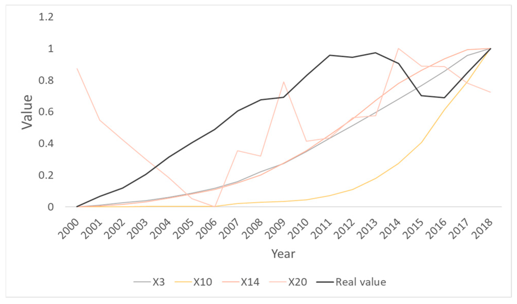
We chose key factors and highly correlated factors as explanatory variables to predict railway freight demand. That is, we excluded $X_3$, $X_{10}$, $X_{14}$, and $X_{20}$. This result is consistent with our expectations with respect to the actual situation. Railway freight primarily consists of bulk commodities, with coal being the main source of railway freight, while small parcel delivery is mainly reliant on road and air transportation. The selection of explanatory variables using GRA is largely consistent with the results obtained from Spearman correlation analysis and Pearson correlation analysis. Additionally, GRA gives more accurate screening results for some specific indicators.

3.3.2. Forecast Results Analysis

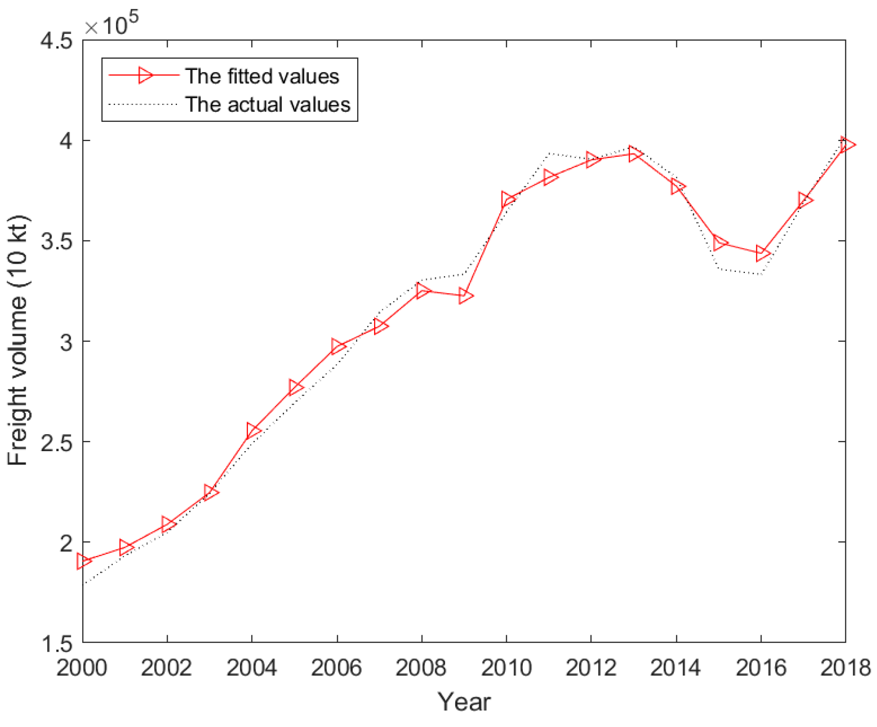
DAE-NN was trained with 2000–2017 data and predicted with 2018 data. The fitting and prediction results are shown in Figure 5. The fitting prediction results are shown in

Table 5. The GRA-DAE-NN model forecast results.

Year		Real Value (Million Tons)	Fitting Value (Million Tons)	Absolute Error (Million Tons)	Relative Error (%)
learning sample	2000	1785.81	1905.94	120.13	6.73%
	2001	1931.89	1974.28	42.39	2.19%
	2002	2049.56	2089.23	39.67	1.94%
	2003	2242.48	2246.98	4.5	0.20%
	2004	2490.17	2554.49	64.32	2.58%
	2005	2692.96	2769.64	76.68	2.85%
	2006	2882.24	2973.19	90.95	3.16%
	2007	3142.37	3074.19	68.18	2.17%
	2008	3303.54	3250.96	52.58	1.59%
	2009	3333.48	3225.78	107.7	3.23%
	2010	3642.71	3705.18	62.47	1.72%
	2011	3932.63	3814.85	117.78	2.99%
	2012	3904.38	3901.8	2.58	0.07%
	2013	3966.97	3931.83	35.14	0.89%
	2014	3813.34	3770.43	42.91	1.13%
	2015	3358.01	3489.44	131.43	3.91%
	2016	3331.86	3436.69	104.83	3.15%
	2017	3688.65	3700.59	11.94	0.32%
predicted	2018	4026.31	3976.89	49.42	1.23%

.

It can be observed from Figure 5 that the GRA-DAE-NN model provides a good fit for predicting railway freight demand. The trained network is validated using the freight volume data from 2018, resulting in a predicted value of 3976.89 million tons with a mean absolute percentage error of 1.23% and a mean fit relative error of 2.21%. These low relative error values show high predictability.

3.3.3. Results Comparison between GRA-DAE-NN and Baseline Models

The GRA-DAE-NN model is compared with the following baseline models:

(1)

ARIMA (autoregressive integrated moving average): ARIMA regards the data series formed by the prediction object over time as a random sequence and uses a certain mathematical model to approximate the series [39];

(2)

SVR (support vector regression): SVR is a time series model that uses the relationship between historical and future data to predict future data [40];

(3)

GRU (gated recurrent unit): GRU is a learning algorithm based on a recurrent neural network, which has a sequence-to-sequence structure and is usually used for time series analysis [41];

(4)

FC-LSTM (fully connected LSTM): It is a classic RNN that learns time series and predicts through fully connected neural networks. In this paper, the hidden layer is set to be two layers; the hidden units are 32 and 64, respectively, the learning rate is 0.001, and the batch size is 64 [42];

(5)

DNN (deep neural network): It uses DNN to extract railway freight demand characteristics and predict railway freight demand [43];

(6)

FNN (feedforward neural networks): FNN is the most basic type of neural network, consisting of an input layer, hidden layer, and output layer, suitable for most classification and regression problems [44];

(7)

GRNN (general recurrent neural networks): GRNN calculates the correlation density function between variables and carries out regression, making it suitable for time series prediction [45].

The results of GRA-DAE-NN and baseline models are shown in

Table 6. Comparison of performance between GRA-DAE-NN and baseline models.

Approach	MAPE (%)	MAE (Million Tons)	RMSE (Million Tons)
ARIMA	5.96%	173.97	189.20
SVR	4.62%	134.86	142.86
GRU	6.94%	202.58	223.76
FC-LSTM	3.35%	78.60	81.63
DNN	4.68%	107.42	111.42
FNN	7.42%	216.59	254.41
GRNN	2.68%	74.23	79.62
The improved GRA-DAE-NN	2.21%	64.51	74.98

.

Compared with the baseline model FC-LSTM with the greatest precision, the GRA-DAE-NN model shows a 1.14% reduction in MAPE, 14.09 in MAE, and 6.65 in RMSE. Compared with the original DNN model, the GRA-DAE-NN model demonstrates a decrease of 2.47% in MAPE, 42.91% in MAE, and 36.44% in RMSE. Compared with ARIMA, SVR, GRU, FC-LSTM, DNN, FNN, and GRNN, the improved GRA-DAE-NN showed a decrease in MAPE of 3.75%, 2.41%, 4.73%, 1.14%, 2.47%, 5.21%, and 0.47%, respectively. Therefore, compared with other prediction models, the improved GRA-DAE-NN model in this chapter exhibits significant forecasting advantages using the same dataset.

3.3.4. Ablation Study

In order to further verify the effectiveness of the proposed model, this chapter designs ablation experiments. In the ablation experiment, we trained and tested prediction models with and without the GRA module on the same dataset. The prediction model without the GRA module was unable to perform selection on the initial set of railway freight demand-related factors. Therefore, we used all 22 variables as explanatory inputs for the model. The verification results are shown in

Table 7. GRA ablation experimental results.

Year		Real Value (Million Tons)	Relative Error (%)
			GRA-DAE-NN	DAE-NN
learning sample	2000	1785.81	6.73%	12.92%
	2001	1931.89	2.19%	3.35%
	2002	2049.56	1.94%	2.31%
	2003	2242.48	0.20%	0.27%
	2004	2490.17	2.58%	2.41%
	2005	2692.96	2.85%	3.43%
	2006	2882.24	3.16%	3.72%
	2007	3142.37	2.17%	1.30%
	2008	3303.54	1.59%	3.05%
	2009	3333.48	3.23%	0.99%
	2010	3642.71	1.72%	2.72%
	2011	3932.63	2.99%	3.82%
	2012	3904.38	0.07%	0.11%
	2013	3966.97	0.89%	0.97%
	2014	3813.34	1.13%	4.77%
	2015	3358.01	3.91%	6.03%
	2016	3331.86	3.15%	6.62%
	2017	3688.65	0.32%	0.82%
predicted	2018	4026.31	1.23%	4.40%
Average		-	2.21%	3.37%

.

As shown in the above table, the GRA-DAE-NN model demonstrates higher prediction accuracy compared with the DAE-NN model. The former has a mean absolute percentage error (MAPE) of 2.21%, while the latter has a MAPE of 3.21%. In terms of fitting historical data, the DAE-NN model only exhibits smaller errors for the years 2004, 2005, 2007, and 2009. The main difference between these two models lies in whether the GRA module is used to filter the explanatory variables. Figure 6 shows the weakly correlated factors removed by the GRA module, in contrast to the trend in rail freight demand.

The aforementioned variables have a small contribution to the trend of railway freight demand. These variables are “Total retail sales of consumer goods,” “Express delivery volume of the year,” “Investment in fixed assets in railway transportation,” and “Number of railway employees.” From the perspective of the railway transportation industry, the main source of railway freight in China is bulk goods. Retail goods and express deliveries are less commonly transported by railways. In recent years, most fixed asset investments have been focused on the construction of high-speed railway lines, which are primarily used for passenger transportation. The number of railway employees includes multiple departments such as operations, mechanical, engineering, electrical, and vehicles, and it does not directly reflect the operational situation of the freight department. The screening results of the GRA module align with the actual situation of railway transportation.

Furthermore, from the perspective of data characteristics, the explanatory variables in the above figure exhibit significant differences from the target variable. During the training of the prediction model, irrelevant features and noise can easily interfere, affecting the accuracy of the model. Therefore, the ablation experiment validates the importance of the GRA module in the GRA-DAE-NN model.

3.3.5. Explanatory Variable Analysis

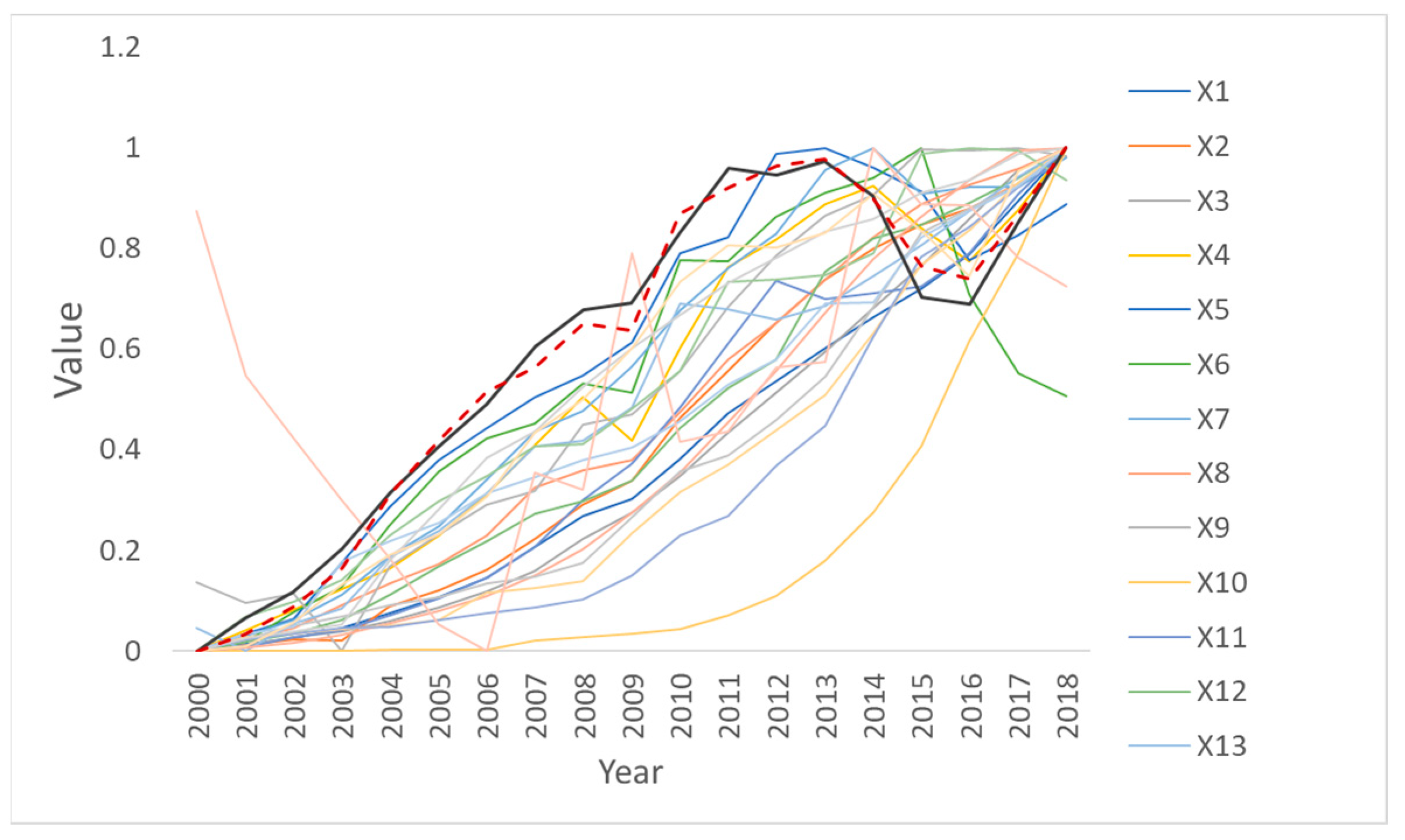
The trend of the actual values and predicted values of railway freight demand, as well as the trend of all explanatory variables data, are shown in Figure 7.

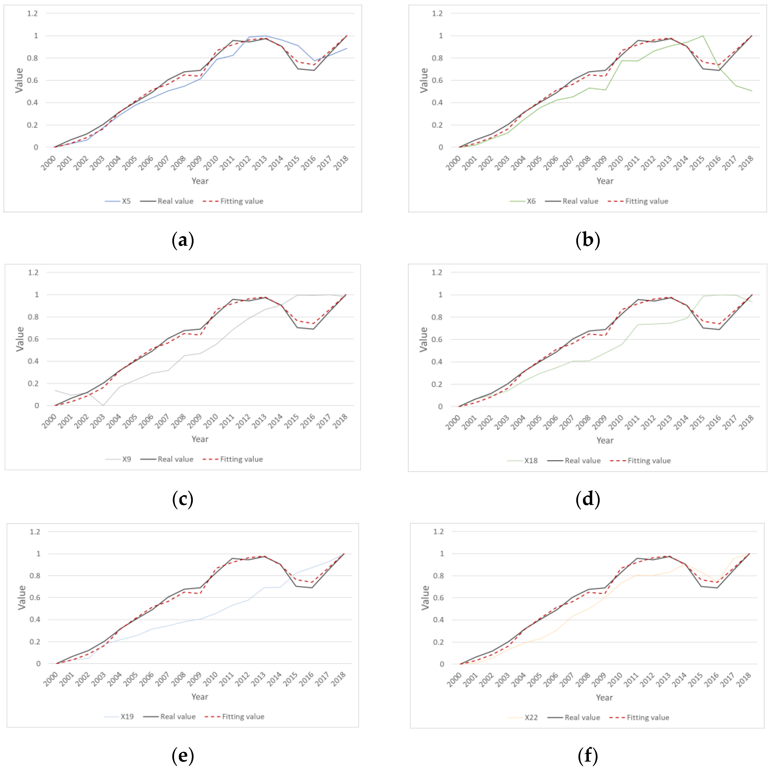
From Figure 7, the factors ($X_3$, $X_{10}$, $X_{14}$, and $X_{20}$) do not adequately account for the changing demand for rail freight. In order to have a clearer observation of the impact of explanatory variables on the trend of railway freight demand, we only select strongly correlated explanatory variables ($X_5$, $X_6$, $X_9$, $X_{18}$, $X_{19}$, and $X_{22}$), and their data trends are shown in Figure 8.

Based on Figure 8, the explanatory variables “Coal production”, “Petroleum production”,“Grain production”, “National railway locomotive inventory”, “National railway freight wagon inventory,” and “Daily production of freight locomotives” have the greatest impact on railway freight demand. In particular, “Coal production”, “Petroleum production”, and “Daily production of freight locomotives” show a nearly consistent trend with the changes in railway freight demand.

Decision-makers may select explanatory variables based on different forecast objectives to provide more accurate forecasts of rail freight demand. In practice, railway freight encompasses a wide variety of goods, each with different transportation demands. The method proposed in this study can not only predict the overall demand for railway freight but also target the demand for a specific category of goods. By adjusting the explanatory variables through the GRA module, different types of goods can be precisely forecasted. At the same time, decision-makers can not only utilize the GRA-DAE-NN model to forecast railway freight demand but also adjust transportation resources, railway routes, locomotives, freight wagons, and strategies for organizing the source of goods by analyzing the quantitative and qualitative relationship between the trend of railway freight demand and the trend of explanatory variables.

4. Conclusions

The article presents a supervised learning GRA-DAE-NN prediction model for analyzing explanatory variables of railway freight transportation and predicting its demand. By combining GRA with the DNN model, explanatory variables relevant to railway freight demand prediction are obtained using GRA, and the feature correlation between these variables and railway freight demand is learned through the DNN model. Additionally, the DAE is introduced to improve the GRA-DNN model, which gives the GRA-DAE-NN model. DAE compresses high-dimensional explanatory variables and adaptively learns data features. Then, it predicts railway freight demand by adding a supervised learning fitting layer. This approach overcomes challenges encountered by the GRA-DNN model, such as the difficulty of extracting high-dimensional data characteristics and the great complexity of calculations. This approach helps decision-makers better understand the reasons for demand trend alterations by observing the changes in explanatory variables, thereby improving the accuracy of response strategies such as transport resource allocation and source matching and has better accuracy and interpretability. The main findings are as follows:

• The improved GRA-DAE-NN model has high predictive accuracy and interpretability for predicting the trend of target changes and can select explanatory variables related to railway freight demand for better prediction. It can not only accurately predict the trend of changes in railway freight demand but also determine the key factors and contribution priorities that affect its changes;
• According to the analysis of the influencing factors by GRA, the core indicators in the explanatory variables for railway freight demand prediction, such as coal production, petroleum production, grain production, daily production of freight locomotives, etc., have the best explanatory power for the trend changes in railway freight demand. Railway policymakers can focus on these indicators to adjust their transportation organization strategies in response to changing demand;
• Through a case study of the Chinese railway freight market from 2000 to 2018 and comparisons with other mainstream prediction models, it is found that the improved GRA-DAE-NN model has higher prediction accuracy. The prediction accuracy of the GRA-DAE-NN model is 97.79%, higher than that of other models such as ARIMA, SVR, FC-LSTM, DNN, FNN, and GRNN, which have prediction accuracies of 94.04%, 95.38%, 96.65%, 95.52%, 92.58%, and 97.32%, respectively. The ablation experiment confirmed the efficiency of the GRA module. After using GRA to filter the explanatory variables, the prediction model exhibited greater precision.

However, certain limitations and gaps are present in this study. The proposed GRA-DAE-NN model depends to a large extent on explanatory variables. In practical applications, the combination of Internet-based data collection methods to build a larger pool of applicants can improve model performance. Additionally, the use of fine-grain data may require refinement of the model. Finally, the inclusion of data on flows of basic explanatory variables between commodity regions may provide more detailed prediction results.

References

1. Brkić, R.; Adamović, Ž.; Bukvić, M. Modeling of Reliability and Availability of Data Transmission in Railway System. Adv. Eng. Lett. 2022, 1, 136–141. [Google Scholar] [CrossRef]
2. Zhang, D.L.; Peng, Y.J.; Xu, Y.; Du, C.Y.; Zhang, Y.M.; Wang, N.; Chong, Y.H.; Wang, H.W.; Wu, D.H.; Liu, J.T. A high-speed railway network dataset from train operation records and weather data. Sci. Data 2022, 9, 244. [Google Scholar] [CrossRef]
3. Xu, G.M.; Zhong, L.H.; Wu, R.F.; Hu, X.L.; Guo, J. Optimize train capacity allocation for the high-speed railway mixed transportation of passenger and freight. Comput. Ind. Eng. 2022, 174, 108788. [Google Scholar] [CrossRef]
4. Tian, Z.D.; Li, S.J.; Wang, Y.H.; Sha, Y. A prediction method based on wavelet transform and multiple models fusion for chaotic time series. Chaos Solitons Fractals 2017, 98, 158–172. [Google Scholar]
5. Luo, Y.; Cai, H.X.; Mao, Y.; Ding, Y.; Zhao, X.Q.; Wei, Z. Enhanced Smith predictor by Kalman filter prediction for the charge-coupled device-based visual tracking system. Opt. Eng. 2022, 61, 054107. [Google Scholar] [CrossRef]
6. Hina, H.; Abbas, F.; Qayyum, U. Selecting correct functional form in consumption function: Analysis of energy demand at household level. PLoS ONE 2022, 17, e0270222. [Google Scholar] [CrossRef]
7. Y, N.N.; Ly, T.V.; Son, D.V.T. Churn prediction in telecommunication industry using kernel Support Vector Machines. PLoS ONE 2022, 17, e0267935. [Google Scholar] [CrossRef]
8. Binhimd, S.; Almalki, B. Bootstrap prediction intervals. Appl. Math. Sci. 2018, 12, 841–848. [Google Scholar] [CrossRef]
9. Kandasamy, A.; Sundaram, M. Content Based Image Retrieval using Modified Histogram with user Feedback Wavelet Analysis Method. Int. J. Comput. Inf. Technol. 2021, 2, 13. [Google Scholar]
10. Gao, Y. Prediction Strategy Method of Short-term Network Public Opinion Based on Improved Chaos Theory. J. Chongqing Univ. Technol. (Nat. Sci.) 2019, 33, 171–176. [Google Scholar]
11. Iwana, B.K.; Uchida, S. An empirical survey of data augmentation for time series classification with neural networks. PLoS ONE 2021, 16, e0254841. [Google Scholar] [CrossRef]
12. LeCun, Y.; Bengio, Y.; Hinton, G. Deep learning. Nature 2015, 521, 436–444. [Google Scholar] [CrossRef]
13. Gao, H.; Yang, W.X.; Wang, J.W.; Zheng, X.Y. Analysis of the Effectiveness of Air Pollution Control Policies Based on Historical Evaluation and Deep Learning Forecast: A Case Study of Chengdu-Chongqing Region in China. Sustainability 2021, 13, 206. [Google Scholar] [CrossRef]
14. Alshboul, O.; Shehadeh, A.; Almasabha, G.; Almuflih, A.S. Extreme Gradient Boosting-Based Machine Learning Approach for Green Building Cost Prediction. Sustainability 2022, 14, 6651. [Google Scholar] [CrossRef]
15. An, G.Q.; Jiang, Z.Y.; Chen, L.B.; Cao, X.; Li, Z.; Zhao, Y.Y.; Sun, H.X. Ultra Short-Term Wind Power Forecasting Based on Sparrow Search Algorithm Optimization Deep Extreme Learning Machine. Sustainability 2021, 13, 10453. [Google Scholar] [CrossRef]
16. Tanner-Smith, E.E.; Tipton, E. Robust variance estimation with dependent effect sizes: Practical considerations including a software tutorial in Stata and SPSS. Res. Synth. Methods 2014, 5, 3–30. [Google Scholar] [CrossRef]
17. Wu, W.T.; Li, P.; Liu, R.H.; Jin, W.Z.; Yao, B.Z.; Xie, Y.Q.; Ma, C.X. Predicting peak load of bus routes with supply optimization and scaled Shepard interpolation: A newsvendor model. Transp. Res. Part E—Logist. Transp. Rev. 2020, 142, 102041. [Google Scholar] [CrossRef]
18. Wu, W.T.; Xia, Y.S.; Jin, W.Z. Predicting Bus Passenger Flow and Prioritizing Influential Factors Using Multi-Source Data: Scaled Stacking Gradient Boosting Decision Trees. IEEE Trans. Intell. Transp. Syst. 2021, 22, 2510–2523. [Google Scholar] [CrossRef]
19. Huang, C.Y.; Hsu, C.C.; Chiou, M.L.; Chen, C.L. The main factors affecting Taiwan’s economic growth rate via dynamic grey relational analysis. PLoS ONE 2020, 15, e0240065. [Google Scholar] [CrossRef]
20. Wang, M.; Wang, W.; Wu, L.F. Application of a new grey multivariate forecasting model in the forecasting of energy consumption in 7 regions of China. Energy 2022, 243, 123024. [Google Scholar] [CrossRef]
21. Wu, L.F.; Gao, X.H.; Xiao, Y.L.; Yang, Y.J.; Chen, X.N. Using a novel multi-variable grey model to forecast the electricity consumption of Shandong Province in China. Energy 2018, 157, 327–335. [Google Scholar] [CrossRef]
22. Huang, Y.S.; Shen, L.; Liu, H. Grey relational analysis, principal component analysis and forecasting of carbon emissions based on long short-term memory in China. J. Clean. Prod. 2019, 209, 415–423. [Google Scholar] [CrossRef]
23. Huang, S.Q.; Xu, H.L.; Liu, C.J. Application of Electro-Optic Rotary Encoder in Automatic Production Line. Adv. Disp. 2006, 11, 63–65. [Google Scholar]
24. Dai, Y.; Ji, E.; Yao, Y. Stacked Auto-Encoder Driven Automatic Feature Extraction for Web-Enabled EEG Emotion Recognition. In Proceedings of the 2021 7th Annual International Conference on Network and Information Systems for Computers (ICNISC), Guiyang, China, 23–25 July 2021; pp. 991–997. [Google Scholar]
25. Wang, H.; Wu, Z.; Xing, E.P. Removing Confounding Factors Associated Weights in Deep Neural Networks Improves the Prediction Accuracy for Healthcare Applications. In Proceedings of the Pacific Symposium on Biocomputing, Kohala Coast, HI, USA, 3–7 January 2019. [Google Scholar]
26. Zhang, L.; Luo, H.; Hu, S.S.; Wang, J.; Kou, Z. Application of Sparse Automatic Encoder in Error Prediction of Multidimensional Electric Energy Metering. Process Autom. Instrum. 2018, 39, 28–31. [Google Scholar]
27. Cao, H.; Chen, L.; Si, J.B.; Ren, J.L. Singular Value Decomposition and Sparse Automatic Encoder for Bearing Fault Diagnosis. Comput. Eng. Appl. 2019, 55, 257–262. [Google Scholar]
28. Wu, L.M.; Lu, J.B.; Liu, C.X. A Recommendation Algorithm Based on Denoising Autoencoders. Comput. Mod. 2018, 3, 78–82. [Google Scholar]
29. Teruna, C.; Avallone, F.; Casalino, D.; Ragin, D. Numerical investigation of leading-edge noise reduction on a rod-air Petroleum configuration using porous materials and serrations. J. Sound Vib. 2020, 494, 115880. [Google Scholar] [CrossRef]
30. Singh, S.K.; Goyal, A. A Stack Autoencoders Based Deep Neural Network Approach for Cervical Cell Classification in Pap-Smear Images. Recent Adv. Comput. Sci. Commun. 2021, 14, 62–70. [Google Scholar] [CrossRef]
31. Uzen, H.; Turkoglu, M.; Hanbay, D. Multi-dimensional feature extraction-based deep encoder-decoder network for automatic surface defect detection. Neural Comput. Appl. 2022, 35, 3263–3282. [Google Scholar] [CrossRef]
32. Khouloud, S.; Ahlem, M.; Fadel, T.; Amel, S. W-net and inception residual network for skin lesion segmentation and classification. Appl. Intell. 2022, 52, 3976–3994. [Google Scholar] [CrossRef]
33. Yang, H.; Huang, C.; Wang, L.; Luo, X. An Improved Encoder-Decoder Network for Ore Image Segmentation. IEEE Sens. J. 2021, 21, 11469–11475. [Google Scholar] [CrossRef]
34. Song, W.; Zhang, Y.X.; Park, S.C. A novel deep auto-encoder considering energy and label constraints for categorization. Expert Syst. Appl. 2021, 176, 114936. [Google Scholar] [CrossRef]
35. Geng, L.; Zhang, T.; Zhao, P. Prediction of LS-SVM Railway Freight Volume Based on Grey Correlation Analysis. J. Railw. 2012, 34, 1–6. [Google Scholar]
36. Cai, B.; Xia, J. A novel artificial neural network method for biomedical prediction based on matrix pseudo-inversion. J. Biomed. Inform. 2014, 48, 114–121. [Google Scholar] [CrossRef] [Green Version]
37. Besinovic, N. Resilience in railway transport systems: A literature review and research agenda. Transp. Rev. 2020, 40, 457–478. [Google Scholar] [CrossRef]
38. Li, Q.L.; Rezaei, J.; Tavasszy, L.; Wiegmans, B.; Guo, J.; Peng, Q. Customers’ preferences for freight service attributes of China Railway Express. Transp. Res. Part A Policy Pract. 2020, 142, 225–236. [Google Scholar] [CrossRef]
39. Saxena, A.; Yadav, A.K. Examining the Effect of COVID-19 on rail freight volume and revenue using the ARIMA forecasting model and assessing the resilience of Indian railways during the pandemic. Innov. Infrastruct. Solut. 2022, 7, 348. [Google Scholar] [CrossRef]
40. Wang, T. An Intelligent Passenger Flow Prediction Method for Pricing Strategy and Hotel Operations. Complexity 2021, 2021, 5520223. [Google Scholar] [CrossRef]
41. Yu, J. Short-term Airline Passenger Flow Prediction Based on the Attention Mechanism and Gated Recurrent Unit Model. Cogn. Comput. 2022, 14, 693–701. [Google Scholar] [CrossRef]
42. Lin, S.; Tian, H. Short-Term Metro Passenger Flow Prediction Based on Random Forest and LSTM. In Proceedings of the 2020 IEEE 4th Information Technology, Networking, Electronic and Automation Control Conference (ITNEC), Chongqing, China, 12–14 June 2020. [Google Scholar]
43. Yang, X.; Xue, Q.C.; Ding, M.L.; Wu, J.J.; Gao, Z.Y. Short-term prediction of passenger volume for urban rail systems: A deep learning approach based on smart-card data. Int. J. Prod. Econ. 2021, 231, 107920. [Google Scholar] [CrossRef]
44. Saadaoui, F.; Saadaoui, H.; Rabbouch, H. Hybrid Feedforward ANN with NLS-based regression curve fitting for US air traffic forecasting. Neural Comput. Appl. 2020, 32, 10073–10085. [Google Scholar] [CrossRef]
45. Guo, Z.D.; Fu, J.Y. Prediction Method of Railway Freight Volume Based on Genetic Algorithm Improved General Regression Neural Network. J. Intell. Syst. 2019, 28, 835–848. [Google Scholar] [CrossRef]
Figure 1. Deep learning model structure.
Sustainability 15 09652 g001
Figure 2. The improved DAE-NN model structure.
Sustainability 15 09652 g002
Figure 3. The process of the GRA-DAE-NN prediction model.
Sustainability 15 09652 g003
Figure 4. The DAE-NN model training process.
Sustainability 15 09652 g004
Figure 5. Railway freight demand prediction results based on the GRA-DAE-NN.
Sustainability 15 09652 g005
Figure 6. Weakly correlated explanatory variables eliminated by the GRA module.
Sustainability 15 09652 g006
Figure 7. Comparison of trends between railway freight demand and explanatory variables.
Sustainability 15 09652 g007
Figure 8. Trends of railway freight demand and strongly correlated variables. (a) Trends in coal production, (b) Trends in petroleum production, (c) Trends in grain production, (d) Trends in national railway locomotive inventory, (e) Trends in national railway freight wagon inventory, (f) daily production of freight locomotives.
Sustainability 15 09652 g008