A Resource Nexus Analysis Methodology for Quantifying Synergies and Trade-Offs in the Agricultural Sector and Revealing Implications of a Legume Production Paradigm Shift

Abstract

Resource management in the sustainability context has increasingly been a key object that makes the application of holistic approaches an imperative need. The water–energy–food nexus concept offers tools for such system analysis in an integrated manner, through the identification and quantification of synergies and trade-offs. The agricultural sector often constitutes one of the main resource depletion hotspots. In this article, a nexus assessment methodological approach is developed for an agricultural context. Water, energy, food, land uses, and greenhouse gas emissions are perceived as nexus components. The methodology considers resource uses within and outside the biogeographical system boundaries, interpreting them as direct and indirect interlinkages. The methodology is validated on an actual case study, in Thessaly, Central Greece. Four nexus indicators are introduced to assess the impact of different land use planning scenarios. Legume production, which has been considered as a relatively beneficial land use among other crop choices, is tested against the four nexus indicators. Multiple advantages of such a land use paradigm shift are revealed, specific to the directions of food security, energy security, and economic sustainability.

1. Introduction

Inequality between developed and developing countries, first seen in the Enlightenment and the Industrial Revolution—or even earlier, by the beginning of the modern era [1,2]—involves implications in economic growth, natural resource depletion, pollution, education, food security, among many other subsystems [3], which according to recent studies of the Sustainable Development Goals (SDGs), are thoroughly interlinked, mostly through synergies, meaning that improvement in one SDG is most likely to drive an improvement in another one [4]. According to the analysis performed by [5], one-seventh of the world’s population does not have access to nutritious food, clean water, and energy resources. At the same time, human activities consume natural resources, leading to the degradation of land and aquatic ecosystems and the services they provide [5]. Climate crisis, urbanization, shifting lifestyles, and policies constitute a complex system of pressures on resource availability [6]. Researchers and policymakers understand the necessity of a holistic and integrated approach to tackle these pressures.

Agriculture has historically been one of the major economic activities that play a key role in shaping Europe’s landscape, as well as the rest of the world. Farming is the most prevailing land use in the 27 countries comprising the European Union, with 172 million hectares of land used for agriculture [7]. Traditional farm management has rapidly transitioned to an industrialized form of agriculture due to the intensification of farming practices. Farm specialization, the use of chemical products, and the systematical use of machinery have stressed biodiversity across Europe’s agricultural area. Nutrient emissions due to farm practices have negative effects on soils, such as contamination of groundwater and less productive land [8] and on surface water ecosystems, causing eutrophication incidents [9]. Agriculture is a major water consumer, first or second depending on the development level of industry [10]. While projections state that water demand for agricultural activities will grow by 55% in 30 years [11], at the same time, agriculture is exposed to climate change stresses, such as shifts in precipitation patterns. This contradiction increases societal vulnerabilities related to food security [12]. Agricultural production is a vital part of the food supply chain, which consumes 30% of the total energy and produces a 20% share of greenhouse gasses (GHGs) at a global scale [13]. The current dietary patterns require increased processing of products, also entailing great amounts of energy consumption for transportation, as well as for their chains within industries. As a result, dietary patterns play an important role in how the supply chain is dependent on energy consumption [14]. In addition to the interlinkages of food and water sectors on the one hand and food and energy on the other hand, the water and energy sectors are also inextricably interlinked. Indicatively, the water sector consumes energy for pumping groundwater, water treatment, desalination, and water distribution, through water networks, in farm sites and cities. In contrast, the energy sector consumes great amounts of water, mostly for energy generation and cooling [15].

The aforementioned constitute only a few of the many interlinkages between the three sectors. A nexus approach has been used to describe the interrelations and interlinkages between the water, energy, and food systems [16]. The interdependencies among the nexus subsystems are dynamic. The challenges of managing one resource, e.g., water, could potentially affect the other resources, e.g., energy or food [17]. There is a need to understand these convolutions, because the interconnectedness of these systems may lead to new societal challenges and reveal innovative multipurpose solutions [18]. The nexus approach has evolved to not be restricted only to water, energy, and food systems; it also includes a wide range of different commodities such as land use, waste, environment, health, and economy [15]. Indicatively, the Sim4Nexus project, which had already included land use and climate change as nexus components, has concluded that integrating an ecosystem dimension into the nexus approach improves the inclusiveness of the methodology [14].

The nexus approach implies the necessity of transdisciplinary research, which has already been incorporated in nexus analysis [14]; however, it focuses on the perspectives of various academics concerning the different nexus components, with the involvement of stakeholders, often limited to the role of end-users. It is well known that stakeholders interact with nexus issues in many ways, and their collaboration within the nexus research can solidify its application and operationalization. Participation of stakeholders could potentially counter the overestimation of macro-level resource availability to provide a more inclusive representation of nexus challenges [19].

Greening the common agricultural policy (CAP) has been a central objective of the EU planning in regard to improving natural resource management, i.e., water, energy, nutrient balances, soil, water quality, biodiversity preservation, food security, and minimization of carbon footprint [20]. Garrod [7] suggested that the exploitation of local expertise operates as a catalyst in sustainable agriculture. Greening the CAP through both its top-down (legislation and incentives) and bottom-up (co-creation and co-design) processes is inextricably linked to a rather extended nexus approach involving not only water, energy, and food dimensions but also land use, nutrients, climate change, soil, ecosystems, and biodiversity.

An important part of the bottom-up approach in sustainable agriculture planning could be that of scoping traditional agricultural paradigms that have been calibrated by societies throughout the years. For example, in the Mediterranean region, legume production has been part of the region’s culture since ancient times [21]. Legume cultivation has been considered to have beneficial effects on the water budget and nitrogen fixation; at the same time, legumes are rich in protein, enhancing regional food security.

Ecosystem services are supported by the natural characteristics of legume crops in multiple ways. Their ability to fix nitrogen, especially in synergy with their bacteria symbionts, facilitates the nitrogen cycle, enriches soils with N-nutrients, and assists the growth of the following crops on the same land. This mechanism decreases the demand for fertilizers for legumes and next cultivations; thus, it decreases nitrogen depletion and the associated carbon footprint and resource consumption of fertilizer production [22]. As reported by Von Richthofen et al. [23], European farmers stated that wheat grown after legume production produced more yield than that grown after cereals. Legumes are known also for their high protein capacity for use as forage for livestock or as food in the form of seeds [21]. Studies based on life cycle assessment (LCA) methods indicate that the preference for legumes as livestock feed offers a series of advantages, including the decrease in the carbon footprint of the production chains, e.g., a 15% decrease in GHG emissions of milk product chains, and improved nutritiousness for several animal species, such as ruminants [24]. Lastly, pulses have less water demand compared to many irrigable crop choices in European countries, such as cotton [6].

The purpose of this study is to clarify the interrelationships between different resource systems in agriculture, through a water–energy–food nexus approach, and reveal the potential benefits of adopting the nexus approach towards sustainable agriculture planning in a holistic manner. The methodology introduces two modes of analysis: (a) a nexus assessment that considers only impacts within the geographical boundaries of the system and (b) a nexus assessment that exhaustively considers all relevant impacts, internal and external to the geographical boundaries, directly and indirectly linked to the procedures taking place. These two modes can serve different objectives. The first assessment is more related to the interests of the farmers, while the second offers a more holistic insight. Such differentiation builds on past nexus studies, such as that of Laspidou et al. [6], offering an approach for more individualized, thus efficient, stakeholder engagement. Different crop scenarios have been tested to investigate if a shift to legume production is a nexus-wise option and quantify any beneficial effect. To this end, an actual agricultural site in Central Greece is selected as the study’s focus area, as the involved agricultural cooperative participated in the design of the nexus map and the quantification of nexus interlinkages through a participatory process. For the facilitation of a deeper understanding of nexus interlinkages, this study introduces four nexus indicators that reveal four different kinds of efficiency: (a) food security, (b) protein-based food security, (c) energy efficiency, and (d) economic sustainability. The scenarios are tested against all indicators, and the planning procedure is linked to different priorities and informed by the quantification of respective indicators.

2. Materials and Methods

2.1. Case Study Area

Greece is a Mediterranean country of approximately 132,000 km². The sectors contributing most to the national gross domestic product are agriculture and tourism. Thessaly is in Central Greece (Figure 1) and is one of the country’s thirteen administrative regions and one of the fourteen river basin districts (RBDs) [6]. It is characterized as a plain area surrounded by mountainous bodies and the Aegean Sea on its east side. The climate in the western and central regions of Thessaly is characterized as continental, with cold winters and hot summers, while intense temperature changes are observed between the two seasons. The eastern side of Thessaly has a Mediterranean climate. In general, summers are hot and dry, with temperatures of up to 40 °C. Precipitation in the area is unevenly distributed spatially and temporally, while precipitation is rare from June to August [25,26].

The Thessalian Plain is the most productive rural area of Greece. The main crops are cotton, cereals, and corn. Pineios River and its tributaries flow through the whole area of Thessaly with a total catchment area of 9500 km². Pineios water resources are mainly used for agriculture. The intensive and extensive agricultural production on the Thessalian Plain has led to a rise in water demand for irrigation, which in turn has led to the overexploitation of groundwater resources. The synchronization of intense drought periods and groundwater reserve overexploitation has brought about a deterioration in the already burdened water balance of the region [6,27].

The agricultural land of Thessaly corresponds to 14% of the total agricultural land in Greece [28]. Arable land covers 57% of the agricultural land in the region, while pastureland covers 20% [26]. As Thessaly Plain is the most intensively cultivated area in Greece, it requires adequacy of irrigated water, especially in summer months when precipitation is at low levels [6]. The intensification of agricultural activity, excessive use of nutrients and pesticides, and historically poor management have led to the qualitative and—at times—quantitative degradation of Lake Karla. The lake is a valuable ecosystem (Natura site) and also serves as a reservoir for irrigation purposes [29].

The agricultural cooperative THESGI (ΘΕΣγη in Greek, www.thesgi.gr (accessed on 7 May 2023)) involved in the present work is a private entity founded in 2013 and lists 54 farmer members with total arable land of over 20 km². The agricultural activities of the cooperative extend across the whole geographical area of Thessaly. Crops include cereals (maize, wheat, and barley), cotton, legumes (beans), and energy plants (oilseed rape and sunflower).

2.2. Data

Data related to the specifications of the case study were gathered through multiple consultations with the agricultural cooperative. Questionnaires in Greek were distributed to member farmers to collect information on pesticide use, agricultural activity schedules, fertilizers, agricultural machinery, irrigation methods, land uses, energy for pumping, and the depth of the underground aquifer (see Questionnaires S1 and S2).

The Nexus_SDM is a system dynamics modeling tool on the nexus for the national case study of Greece. It was one of the main outcomes of the Sim4Nexus project and was developed on the river basin district scale. The Nexus_SDM was exploited as a database for the current analysis. It provided data for the Thessaly RBD (GR08); specifically, it provided data on water needs for all different crops, precipitation, evapotranspiration, water losses, and parameters related to the irrigation system specifications [30]. The National Meteorological Service (HNMS, Hellenic National Meteorological Service (emy.gr), accessed on 7 May 2023) provided additional required data for the precipitation of the area. Characteristics of the irrigation supply network were provided by Dasberg and Or [31]. The Hellenic Statistical Authority (www.statistics.gr, accessed on 7 May 2023) provided the data relevant to the production of crops. For the application of the LCA of all involved agricultural processes, the Life Cycle Inventories of Agricultural Production Systems publication by Nemecek and Kagi [32] was used.

2.3. Methodology

The design of a conceptual model is a prerequisite for the quantification of interconnections between the nexus dimensions. The conceptual model clearly presents the interconnections between the different agricultural processes that involve resource use. It was designed based on a literature review and information provided by the cooperative and was an outcome of review iterations between the authors and the stakeholders. An overarching version of the conceptual model is presented in Figure 2.

The different nexus dimensions are depicted in different colors. The land uses in brown at the center of the conceptual model represent the agricultural land covers of the different crops of the cooperative. The water component is shown in deep and light blue. Deep blue is used when the water use is direct actual water consumption, within the spatial boundaries of the case study; light blue is used when the water use refers to indirect consumption expressed through the water footprint of involved processes and infrastructure/materials [6,31,33,34,35]. The elements related to energy are represented in deep and light yellow. Deep yellow is used for actual energy consumption, within the spatial boundaries of the case study; light yellow is used for indirect energy uses as revealed by the life cycle assessments implemented for the different materials and processes [32,35]. Greenhouse gas (GHG) emissions are shown in grey. The grey box shows the production of GHGs. GHGs are an indicator of human pressure on climate and a driver of climate change. They are not considered a resource in the conventional way that water and energy are. However, for the needs of our analysis the convention that GHGs are a “reverse resource” is made. While the boxes of the other dimensions denote resource consumption, the grey boxes denote GHG emissions. This means that the emission of GHGs is considered as a pressure in the same way that water consumption is a pressure. Light grey and deep grey are used to show direct GHG emissions in the boundaries of our case study, while light grey is used for GHG emission that is indirect and has occurred outside the boundaries of the case study. This is expressed through the carbon footprint concept [36]. The food dimension is depicted in red and represents the food and fodder production of the agricultural activity of the cooperative. The brown land-use box contains some red boxes that correspond to crops that are used for food production, while the remaining land uses are denoted with light brown, for crops that are not used for food, such as the industrial crop of cotton and the energy crops of rapeseed and sunflower.

The arrows that link the boxes depict the interlinkages between the nexus dimensions. The arrow direction from element A to element B shows the consumption of resource A that is needed for the use of element B. For example, the blue arrow from “crop water needs” to “land uses” shows the consumption of water resources that is needed for agricultural land uses. Following our convention of “reverse resource”, the grey arrows follow a direction from the grey boxes to the yellow ones, showing that GHGs are emitted/produced—and not consumed—for the needs of energy use. Phantom whitish boxes are used to depict some key processes that entail the use of more than one resource.

Land Use–Food (LF): LF would involve the land cover of the different crops for food production (

Table 1. Agricultural land uses cover in km².

Crop	Land Cover (km2)
maize	1.0
wheat	10.0
barley	5.0
beans	0.5
cotton	2.5
rapeseed	0.5
sunflower	0.8

). Other antagonistic agricultural land uses that are not used for food production are also noted to estimate the total irrigation needs for the total of the land uses: The area covered by each of the crops was provided by the cooperative. Maize, wheat, barley, and beans are the crops for food production, while rapeseed, sunflower, and cotton constitute the antagonistic land uses. Apparently, wheat covers almost 50% of the whole area. Food is quantified with the use of a binary expression of protein content in tons and caloric value in kcal [37], taking into account the food and fodder mass production yields of each crop (Hellenic Statistical Authority, 2020) (Figure 3).

Water–Food (WF): The WF flow is perceived as the vector addition of WL + LF.

Water–Land Use (WL): The WL flow involves the precipitation (

Table 2. Precipitation in mm for the reference year of 2020 (source: Hellenic National Meteorological Service).

	Precipitation
JAN	30.9
FEB	19.4
MAR	33.6
APR	57.5
MAY	8.0
JUN	11.3
JUL	2.4
AUG	5.9
SEP	42.4
OCT	24.0
NOV	75.0
DEC	134.7

) that covers part of the water demand (

Table 3. Monthly crop water demand per cultivating area in m³/km² (source: Nexus_SDM, [6]).

	Maize	Wheat	Barley	Rapeseed	Beans	Cotton	Sunflower
JAN	-	-	-	-	-	-	-
FEB	-	-	-	-	-	-	-
MAR	-	-	-	-	-	-	-
APR	0.014	-	-	0.019	-	0.074	0.037
MAY	0.039	-	-	0.069	-	0.099	0.136
JUN	0.188	-	-	0.114	-	0.112	0.223
JUL	0.235	-	-	0.048	0.069	0.121	0.093
AUG	0.071	-	-	-	0.095	0.115	-
SEP	-	-	-	-	0.128	0.093	-
OCT	-	-	-	-	0.120	-	-
NOV	-	-	-	-	-	-	-
DEC	-	-	-	-	-	-	-

), and the crop water needs per land use. The calculation of the actual water needs required for irrigation is the subtraction of precipitation from crop water demand (

Table 4. Monthly crop water needs after subtracting the precipitation per cultivating area in m³.

	Maize	Wheat	Barley	Rapeseed	Beans	Cotton	Sunflower
JAN	-	-	-	-	-	-	-
FEB	-	-	-	-	-	-	-
MAR	-	-	-	-	-	-	-
APR	13,750	-	-	9397	-	41,828	29,328
MAY	30,718	-	-	30,738	-	22,673	102,011
JUN	176,766	-	-	51,438	-	25,222	169,121
JUL	232,719	-	-	22,657	33,090	29,556	72,534
AUG	65,488	-	-	-	44,646	27,205	-
SEP	-	-	-	-	42,892	12,597	-
OCT	-	-	-	-	47,878	-	-
NOV	-	-	-	-	-	-	-
DEC	-	-	-	-	-	-	-

), as the cooperative claimed that irrigation is adjusted to the precipitation patterns. It should be noted that the water needs of wheat and barley crops are zero as they are considered non-irrigated crops. In the case of the agricultural cooperative of this study, a drip irrigation system is used. By adding the estimated water losses through the irrigation system and evapotranspiration to the water needs, the final quantities of groundwater resources that should be pumped are estimated (

Table 5. Monthly total groundwater resources pumped per crop cultivated area in m³.

	Maize	Wheat	Barley	Rapeseed	Beans	Cotton	Sunflower
JAN	-	-	-	-	-	-	-
FEB	-	-	-	-	-	-	-
MAR	-	-	-	-	-	-	-
APR	15,262	-	-	10,431	-	62,241	32,554
MAY	34,097	-	-	34,559	-	253,875	120,336
JUN	196,211	-	-	57,717	-	283,078	197,759
JUL	258,318	-	-	25,281	36,862	328,736	82,644
AUG	72,692	-	-	-	49,882	303,600	-
SEP	-	-	-	-	49,942	151,489	-
OCT	-	-	-	-	54,465	-	-
NOV	-	-	-	-	-	-	-
DEC	-	-	-	-	-	-	-

, Figure 4 and Figure 5).

Two additional indirect water consumptions are estimated: the water footprint for agricultural machinery and the greywater footprint due to the pollution caused by excessive use of fertilizers. The agricultural machinery water footprint is estimated according to Mantoam et al. [38]. The required pieces of machinery used for agricultural purposes were reported by the cooperative; they are associated with the materials used for their manufacturing, maintenance, and repair, and finally, they are assigned a blue water footprint according to material masses (

Table 6. Indices for blue water footprint per material mass.

Material	Blue Water Footprint (lt/kg)
steel	2.5
rubber	6.3
glass	12.5
plastic	23.7
varnish	14.6
other	78.2

), while other water footprints are considered as negligible [38]. The materials used for the analysis are steel, rubber, glass, plastic, varnish, and others, and the masses of each material composing the tractor and other machinery types used by the cooperative were taken from the work of Nemecek et al. [32] (Figure 6). The annual blue water footprint for the machinery is estimated as 181 m³ taking the assumption of a ten-year use of each machine. The machine use per crop is taken as uniform. Regarding the assessment of greywater footprint, the UNESCO-IHE tier 1 supporting guidelines [39] are followed. The greywater footprint is estimated as a function of the pollutant load (L), the maximum acceptable concentration of the pollutant (c_max), and the natural background concentration (c_nat) in the receiving waterbody. The pollutant load, which in this case refers to fertilizers, is estimated as a function of the applied masses reduced by case-specific factors relevant to atmospheric input, soil properties, climate conditions, and agricultural practices [39]. The report includes maps in its appendix that provide estimations of these factors specific to Greece. The cooperative provided data on the type and application mass of fertilizer (

Table 7. Calendar of main agricultural processes for each crop as provided by the cooperative: tillage (T), sowing (S), surface fertilizing (SF), basic fertilizing (BF), Pesticides (P)and harvesting (H). The processes are assumed to take place uniformly during the month, where denoted.

	Maize	Wheat	Barley	Rapeseed	Beans	Cotton	Sunflower
JAN		SF	SF
FEB	T	SF	SF
MAR	S, BF, P			SF, P		BF, T	BF, T
APR						S, BF, P	S, P
MAY	SF	H	H		T		SF
JUN		H		H	S, BF, P	SF
JUL
AUG	H					P	H
SEP					H	H	H
OCT		BF, T	BF, T	T		H
NOV		S	S	S, BF, P
DEC

and

Table 8. Surface and basic fertilizing in kg of urea per 10⁻³ km² as provided by the cooperative.

	Maize	Wheat	Barley	Rapeseed	Beans	Cotton	Sunflower
SF	40	2 × 25	2 × 25	15	0	40	25
BF	40	25	25	15	15	60	40
total	80	75	75	30	15	100	65

). The maximum acceptable concentration is set equal to 0.0113 N kg/m³ by the National Greek legislation, and the natural concentration is taken as zero, which is the safe-side common practice. Though fertilizing (basic and surface) occurs in specific months for each crop, the greywater footprint is estimated as an annual value, since it is naturally attributed to the whole agricultural circle. Moreover, nitrogen is a conservative pollutant, and monthly analysis would not be meaningful in this context [40]. For the monthly analysis of water consumption, the annual value is uniformly distributed to all the months of the agricultural annual circle. The greywater footprint estimation is based on urea and not another pollutant because urea is the prevailing one, since pesticides are applied on the plant and not on the soil. The polluted water due to urea includes greywater of any other pollutant, while it would be an overestimation to assess additional greywater footprints (

Table 9. Greywater footprint in 1000 m³ for each crop.

	Maize	Wheat	Barley	Rapeseed	Beans	Cotton	Sunflower
GWF	351	3295	1647	66	33	1757	228

).

Energy–Water (EW): For the energy-to-water interlinkage, the energy needed for the irrigation system needs to be calculated. The irrigation for the case study is covered by groundwater and is implemented through drip emitters. Thus, the energy consumed needs to cover the pumping from the aquifer level, which is 150 m deep, the transfer losses, and the pressure demand. The estimation of the energy needed for the pumps’ operation is calculated as the power demand (1) [41] multiplied by the pumping hours.

$$P=\frac{h_A \gamma Q}{1000 \eta Dr}$$

(1)

where:

P is the power in KW;

h_A is the pumping depth (150 m);

γ is the water specific weight (=9810 Ν/m³);

Q is the pumping flow rate in m³/s;

η is the pump efficiency (=0.75);

Dr is engine derating (=0.8).

The irrigation system in the case study does not include a tank. This means that the irrigation is conducted at the exact time when the pumps operate. To estimate the pumping hours per 24 h, the flow rate capacity of the farms needs to be divided by the total amount of water demand. The flow rate capacity of each farm is determined by the number of emitters and the standard emitter base flow rate (equal to 1.01 × 10⁻⁶ m³/s) [31]. The number of emitters required per crop type is such that the soil is saturated with water and depends on the surface wetted by each emitter, for the emitters that belong in the same pipeline and corresponding wetted strip, whose radius (r_s = 0.56 cm) is given by Equation (2) and extent (x_s = 0.42 m) is given by Equation (3). For reasons of computational simplification, it is considered that all crops are grown in the same type of soil, which is characterized as between clayey and sandy soils. The minimum distance so that two sprayers, in the same pipeline, do not overlap is equal to 2 r_s. The maximum length of a pipeline is 60 m. By dividing the total length of the pipe by the distance between two sprayers, the number of sprayers of each pipe is calculated. The number of required pipelines is estimated by dividing the total crop area by the pipeline cover area (60 m × 0.42 m = 25.2 m²). Then, the number of emitters for each crop area is estimated as the number of required pipelines multiplied by the number of emitters per pipeline. In

Table 10. Flow rate capacity for each crop of the cooperative.

Crop Area Type	Number of Emitters	Flowrate Capacity (m3/h) = Emitters × Emitter Flow Rate	Total Annual Pumping Time (h) = Flowrate Pumped (m3/h)/Flow Rate Capacity (m3/h)
maize	2,121,409	7721	75
wheat	0	0	0
barley	0	0	0
rapeseed	1,060,731	3861	33
beans	1,060,731	3861	50
cotton	5,303,497	19,304	72
sunflower	1,697,171	6178	70

, the flow rate capacity for each crop area is estimated.

$$r_s=\sqrt{(\frac{4}{a^2\times {\pi }^2}+\frac{q}{\pi \times K_s}}-\frac{2}{a\times \pi }$$

(2)

where $a$ and Ks refer to the type of soil of each crop, with the second variable expressing the permeability of the soil.

$$x_s=\frac{1}{2}\left(\frac{q_l}{K_s}-\frac{3}{4a}\right)$$

(3)

The flow $q_l$ expresses the flow of the whole pipe per unit length of pipe. It is equal to the product of the flow of a sprayer with the number of sprayers on the pipe divided by the length of the pipe. The $q_l$ flow must be less than 3 Ks/4a.

Table 11. Operation pumping hours per crop type per month.

(h)	Maize	Wheat	Barley	Rapeseed	Beans	Cotton	Sunflower
JAN	-	-	-	-	-	-	-
FEB	-	-	-	-	-	-	-
MAR	-	-	-	-	-	-	-
APR	2.0	-	-	2.7	-	3.21	5.3
MAY	4.4	-	-	9.0	-	13.2	19.5
JUN	25.4	-	-	15.0	-	14.7	32
JUL	33.5	-	-	6.6	9.5	17.0	13.4
AUG	9.4	-	-	-	12.9	15.7	-
SEP	-	-	-	-	12.9	7.8	-
OCT	-	-	-	-	14.1	-	-
NOV	-	-	-	-	-	-	-
DEC	-	-	-	-	-	-	-

presents the operation pumping hours for each crop type and per month,

Table 12. Energy consumed for pumping per crop type per month.

(GJ)	Maize	Wheat	Barley	Rapeseed	Beans	Cotton	Sunflower
JAN	-	-	-	-	-	-	-
FEB	-	-	-	-	-	-	-
MAR	-	-	-	-	-	-	-
APR	37	-	-	26	-	153	80
MAY	84	-	-	85	-	623	295
JUN	481	-	-	142	-	694	485
JUL	634	-	-	62	90	806	203
AUG	178	-	-	-	122	745	-
SEP	-	-	-	-	122	372	-
OCT	-	-	-	-	134	-	-
NOV	-	-	-	-	-	-	-
DEC	-	-	-	-	-	-	-

presents the estimated energy consumption for pumping per crop type and per month, and

Table 13. Energy consumed for pumping per crop type per month per km².

(GJ/km2)	Maize	Wheat	Barley	Rapeseed	Beans	Cotton	Sunflower
JAN	-	-	-	-	-	-	-
FEB	-	-	-	-	-	-	-
MAR	-	-	-	-	-	-	-
APR	37	-	-	51	-	61	100
MAY	84	-	-	170	-	249	369
JUN	481	-	-	283	-	278	606
JUL	634	-	-	124	181	322	253
AUG	178	-	-	-	245	298	-
SEP	-	-	-	-	245	149	-
OCT	-	-	-	-	267	-	-
NOV	-	-	-	-	-	-	-
DEC	-	-	-	-	-	-	-
sum	1414			628	938	1357	1328

presents the estimated energy consumption for pumping per crop type, month, and km². Figure 7 and Figure 8 present the total energy consumption distribution per crop type and per month, respectively.

Energy–Land(–Food) and (Food–)Land–Energy Interlinkages: The energy consumed for agricultural land is estimated as direct and indirect components. The direct components refer to the actual amounts of energy that are consumed in the geographical boundaries of a case study and involve fuel for the operation of the agricultural machinery and the energy equivalent for human labor. It is crucial for human labor to be estimated in terms of energy, for reasons of comparison between full-machinery and non-machinery paradigms. In a hypothetical extreme case study, where there is no use of machinery at all and all works are implemented by human labor, this would artificially and falsely introduce the bias that this case is a sustainable paradigm regarding energy use and eventually the nexus. However, it would have neglected human fatigue and the respective energy consumed. The indirect components refer to the energy consumed for the agricultural machinery life cycle, including the phases of assembly, repair and maintenance, and disassembly, as well as the energy demand for producing fertilizers and pesticides. Energy for transferring the machinery, the pesticides, the fertilizers, and the seeds is not estimated, since it would not offer anything in regard to this analysis, since it would add a very case-specific energy amount that would not be generalizable.

In the estimation of fuel consumption, it is considered that the fuel used by agricultural machinery is diesel. The machines at the disposal of the cooperative are agricultural tractors and threshing machines. The data for calculating the diesel fuel consumption of tractors and threshing machines were provided by Nemecek and Kägi [32]. Equation (4) gives the energy consumption of the agricultural machines.

$$E_F=C_{F,mean}\times operation time\times {ED}_D$$

(4)

where $E_F$ (MJ/km²) is energy due to fuel consumption for agricultural field work processes by agricultural machines, $C_{F,mean}$ (m³/h) is the average fuel consumption, operation time (h/km²) is the time required for the agricultural work field processes, and ED_D (MJ/m³) is the energy density of diesel. In

Table 14. Energy consumed by machinery for field work processes.

Crop Area Type	Energy (GJ)	Energy (GJ/km2)
maize	281	281
wheat	4517	452
barley	1522	304
rapeseed	144	289
beans	129	258
cotton	1149	460
sunflower	343	428

, the total energy consumed by agricultural machinery for field work processes is shown.

Research work by Mandal et al. [42], Ozkan et al. [43], and Unakitan et al. [44] gives the energy equivalent of human labor in agricultural works (=1.96 MJ/h/farmer); EUROSTAT gives the average annual work effort for Greece in the agricultural sector (=416.9 h); and the Hellenic Statistical Service gives the number of farmers that work on the agricultural land (=20 farmers/km²). It is assumed that all different crop types demand the same work effort and that the effort is uniformly distributed during the year. The annual energy equivalent for human labor is estimated as being equal to 311 GJ, or 15.3 GJ/km².

The energy consumed in the various phases of the machinery life cycle, for machinery with engine power from 50 hp to 130 hp, is calculated as an indirect energy–land interlinkage. These tractors belong to the category of medium power and are widely used by Greek farmers [45]. The life cycle analysis of a machine includes the phases of assembly, maintenance, and disassembly. For each of these phases, the total energy required is addressed. The estimations are based on the machinery weight and materials: rubber, glass, plastics, various types of varnishes (including paints), and various other materials used to a lesser extent [32]. Mantoam et al. [35] give the energy (Figure 9) and greenhouse gas emission equivalents for the assembly phase of each material. The total assembly energy of the tractor is estimated as being equal to 187,100 MJ. The energy required to repair and maintain the machine is equal to 0.55 times the energy consumed during the assembly phase [46], while for its disassembly, 0.5 MJ per kg of the machine is consumed [32]. The energy demand for the three phases is presented in

Table 15. The total energy consumed for each phase of the tractor life cycle.

Machinery Life Cycle Phase	Energy Demand (GJ)
assembly	187.1
repair and maintenance	102.9
disassembly	1.8
total	291.8
total/month/km2 (for 112 agricultural machines and 10 years of life cycle for each machine)	14

.

The indirect energy–land(–food) interlinkage that refers to fertilizers and pesticides is assessed based on the approaches of Unakitan [44] and Audsley et al. [47]), respectively. The two phases of fertilizer deposition, basic fertilizing and surface fertilizing, are defined and assessed. Basic fertilization is defined as the addition of essential nutrients to the soil before the growing season. Nitrogen is usually given in small, repeated doses. Surface fertilization is the application of nutrients to plants during the period of their growth. The assumption that the application of fertilizers matches the recommended amount would introduce a major error, since producers commonly share the perception that intense use of fertilizers brings the maximum possible harvest, despite environmental risks, such as eutrophication, increased soil acidity, inability to absorb other nutrients from plants, pollution of the aquifer, unwanted growth of parasitic organisms, and greenhouse gas emissions [48,49]. To mitigate such an error, in the assessment of fertilizer and pesticide amounts applied, the actual amounts used by local producers are defined by the cooperative. The equivalent energy index of nitrogen in fertilizers is equal to 66.4 MJ/kg [44], while the fertilizers applied have a nitrogen mass content equal to 46%. Globally, parasites (insects, fungi, weeds) are responsible for the destruction of crops at a rate of 42–48%, before and after harvest. Pesticides and non-chemical biological tests are used for plant protection (crop rotation, cultivation of different species of the same crop) [50]. Due to the growing interest in identifying greenhouse gases, many studies focus on emissions from the manufacture of pesticides. Due to the lack of original data, due to commercial secrecy, many studies show discrepancies in the components of the pesticides. The problem is exacerbated by the rapid change in their composition over time. The global pesticide industry needs to provide reliable numbers that can be used universally [47]. The indirect energy consumption due to pesticides is estimated based on the approach of Audsley et al. [47], who defined the amount of energy (MJ/hectare) required for the plant protection of each crop. Data on the plant protection of all crop cultivation were provided by the cooperative to avoid the introduction of significant errors, similar to the assessment of fertilizer amounts.

Table 16. Indirect energy consumption due to the use of fertilizers and pesticides.

Crop Area Type	Due to Fertilizers		Due to Pesticides		Due to Fert. and Pest.
	(GJ)	(GJ/km2)	(GJ)	(GJ/km2)	(GJ/Km2)
maize	2434	2434	54	54	2488
wheat	22,818	2282	820	82	2364
barley	11,409	2282	406	81	2363
rapeseed	456	913	38	77	990
beans	228	456	32	65	521
cotton	12,169	4868	282	113	4981
sunflower	1582	1978	62	77	2055
total	51,098	-	1694	-	-

shows the total amount of fertilizer- and pesticide-driven indirect energy demand used by the farmers of the cooperative for each crop. There is no assessment of the monthly distribution of the energy consumption, since it does not occur in the geographical boundaries of the case study or at the time of the application; thus, such an assessment is irrelevant to the energy consumption peaks in the agricultural processes.

Table 17. Indirect energy consumption due to the production of seeds used annually during the sowing phase.

Crop Area Type	Energy (GJ/km2)	Energy (GJ)
maize	137	137
wheat	388	3880
barley	320	1600
rapeseed	15	7.5
beans	94	47
cotton	97	973
sunflower	42	34
total	-	6678

presents the annual energy consumed to produce seeds that are used during the sowing phase, according to Elsoragaby et al. [51].

The land–energy interlinkage implies the indirect land demand for energy production through the production of energy crops. This interlinkage is assessed based on the approach of Ralph et al. [52], who used the weight of crop to make fuel (=3.28 kg of raw material/kg of fuel), the energy density of fuel (=43.7 MJ/kg), and the process energy cost for fuel (=0.44 MJ/kg) in the study of oil crops, namely rapeseed and sunflower. For the produced energy crop mass (=390,212 kg), the net energy equivalent is estimated as being equal to 5147 GJ, or 224 GJ/km². Reversely, the land needed to produce energy is 0.0045 km²/GJ.

GHG emissions from energy consumption, the energy–climate Interlinkage: In an agricultural context, crop cultivation land uses do not showcase significant differences in terms of carbon sequestration versus GHG emissions. This would be true if forests or wetlands were included in a context of more extended land use boundaries, or if livestock was one of the agricultural activities. In that case, land use choices would imply a significantly different impact on GHG emissions than on energy consumption. With the selected land use boundaries, the GHG emissions shifts would follow, almost in a flat rate mode, the shifts in energy consumption. For this reason, the GHG emissions estimated are not presented, since they do not introduce any added value to this study and discussion.

For the facilitation of the nexus evaluation of the different crops and the agricultural planning, four indicators are introduced. The first nexus indicator (NI₁, Equation (5)) refers to food production, giving equal priority to the caloric value, the protein value, the water and energy consumption, and the land cover. The second, NI₂ (Equation (6)), prioritizes the protein value of the food product in comparison to the caloric value, the water and energy consumption, and the land cover. It can be used for planning with the objective of protein-based food security. The third nexus indicator (NI₃, Equation (7)) accounts for the economic value of the crops, which can facilitate comparison between food crops, energy crops, and industrial crops. It can be used for planning with the objective of economic sustainability. It should be noted that the prices used for this indicator are taken from the cooperative for the reference year, while for more efficient planning, the dynamic nature of this indicator should be considered. The fourth nexus indicator (NI₄, Equation (8)) accounts for the produced energy from energy crops as biofuel. This indicator facilitates comparison between the energy crops and can be used for prioritizing energy security planning scenarios.

Nexus Indicator 1 focusing on food security:

$${NI}_1=\frac{\sqrt[2]{Caloric value\ast Protein value}}{\sqrt[3]{total Water consumption\ast total Energy consumption\ast Land cover}}$$

(5)

Nexus Indicator 2 focusing on a protein-based food security:

$${NI}_2=\frac{\sqrt[3]{Caloric value\ast {Protein value}^2}}{\sqrt[3]{total Water consumption\ast total Energy consumption\ast Land cover}}$$

(6)

Nexus Indicator 3 focusing on the economy:

$${NI}_3=\frac{Economic value}{\sqrt[3]{total Water consumption\ast total Energy consumption\ast Landcover}}$$

(7)

Nexus Indicator 4 focusing on energy security:

$${NI}_4=\frac{Energy output value}{\sqrt[3]{total Water consumption\ast total Energy consumption\ast Land cover}}$$

(8)

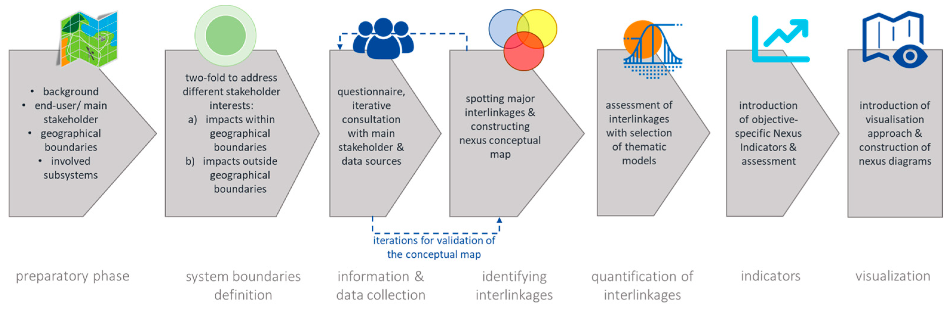
Figure 10 illustrates an overview of the steps followed to conduct the specific nexus analysis of an agricultural context. The steps include (i) the preparatory phase, where the end-user, the case study, and the main systems are identified; (ii) the system boundary definition, where two modes, an internal and an external to the geographical boundaries, are involved to address the concerns of farmers and of a more inclusive audience; (iii) the information and data collection phase; (iv) the interlinkage identification phase, which includes an iterative loop with the previous step; (v) the quantification of interlinkages, where the selection and application of models and empirical equations are conducted; (vi) the introduction and assessment of appropriate indicators, with the use of scenario tests; and (vii) the visualization of results.

3. Results and Discussion

A nexus analysis of an agricultural context implies the assessment of the resources needed to produce the agricultural product, comparing the different crop types regarding the agricultural strategy objectives and priorities, which are linked to the availability of resources. For this reason, all resources are presented as relative values of another nexus component resource, to reveal the benefits and disadvantages in regard to resource use. Figure 11 indicates that sunflower, cotton, and maize consume the most energy regarding direct energy consumption, while cotton consumes by far the most energy also regarding total energy consumption, reaching levels higher than 6500 GJ/km², whereas the crop with the second highest energy consumption is maize, which demands approximately 4200 GJ/km². Regarding food production (Figure 12 and Figure 13), maize consumes the least energy, producing high levels of protein and Kcal, over 0.030 protein tons/GJ and over 0.080 kcal/GJ, while beans come second in protein and barley comes second in Kcal. High protein and Kcal per energy consumption would imply beneficial choices in energy crisis and food security policies. Figure 14 and Figure 15 present the monthly direct and total energy consumption of each crop type per land cover, respectively. Regarding the direct use, energy consumption within the boundaries of the case study, there is a peak of energy use around June and July that is caused by maize, rapeseed, and sunflower, while beans and cotton have a different peak in autumn, offering some separation of energy demand. This can be a beneficial characteristic for the bean energy consumption pattern, since it decongests the July peak, reducing the hazard of blackouts. Total energy consumption has different peaks, but this is not representative of what is the case, because energy consumption outside the case study boundaries, such as the energy demand for producing fertilizers and pesticides, is occurring at different times than what is depicted in the diagrams, considering storage and transportation delays. The largest amounts of energy observed in the energy sector are mainly due to the indirect energy inputs of fertilizers.

Regarding water consumption per land cover, Figure 16 shows that cotton, sunflower, and maize are the most consuming crops regarding direct water use, over 500,000 m³/km², but cotton is much more water-intensive regarding total water use. All the necessary amount of water for their growth is covered through the rain; however, they have significant indirect water demands, over 300,000 m³/km², yet the lowest total. Beans and rapeseed have relatively low direct and indirect water demands. Regarding protein production per water consumption (Figure 17), maize and wheat are the most efficient, and barley and beans follow. Maize has the highest values of Kcal, as well, followed by wheat and barley (Figure 18). The lowest caloric value per water consumption is that of beans. Figure 19 shows that the peak for direct water consumption occurs in the summer, June and July, with maize and sunflower being the greatest drivers. Beans offer the benefit of having a different and smoother peak, almost uniform across the autumn months. This creates relief regarding water consumption in summer, which can be crucial for water deficits in water-scarce regions. Figure 20 follows a pattern similar to that of direct water consumption.

Figure 21, Figure 22 and Figure 23 compare NI_1–3 for the different food crop choices. They show that maize is the most nexus-efficient choice (NI₁ = 0.15,

Table 18. Assessment of the nexus indicators for each crop.

/(Water m3 * GJ * km2)1/3	(Kcal * Protein ton)1/2	(Kcal * (Protein Ton)2)1/3	EUR	GJ
maize	0.15	0.13	222	0.0
wheat	0.07	0.06	95	0.0
barley	0.07	0.06	88	0.0
rapeseed	0.00	0.00	45	6.5
beans	0.06	0.06	528	0.0
cotton	0.00	0.00	105	0.0
sunflower	0.00	0.00	93	4.0

), while wheat, barley, and beans depict almost the same efficiency (NI₁ = 0.07, 0.07, and 0.06, respectively). It should be noted that beans are of comparable nexus efficiency to wheat and barley, even though wheat and barley are rainfed crops. When the protein content is prioritized, maize is the most nexus-efficient (NI₂ = 0.13), again, but wheat, barley, and beans take the same value (0.06). When it comes to economic sustainability, beans are dominantly the most efficient choice with NI₃ equal to 528, followed by maize (222). Rapeseed is less efficient, with NI₃ equal to 45. It should be noted that cotton, which offers neither food security nor energy security, ranks low in the economic sustainability NI, which means that it consumes a lot of water, energy, and land for the economic benefits it brings, compared to the other crops, especially beans and maize which have higher values but also contribute to food security. Lastly, in a comparison of the energy crops, rapeseed (NI₄ = 6.5) shows better efficiency than sunflower (NI₄ = 4.0).

These results are also visualized in the diagrams in Figure 24. Figure 24 schematically depicts the inflows of direct water, total water (including indirect consumption), direct energy, total energy (including indirect consumption), the produced added values in calories, protein, and euros, and the energy outflow regarding the produced energy crops for biofuels. The line widths and the barrel heights follow a scale to facilitate comparison. Specifically for the energy crops, an energy balance is assessed through a net value of direct energy consumption and energy product, and a total net value of total energy consumption (including indirect energy consumption) and energy product. By comparing the two energy crops, sunflower is proven to offer a higher net energy product, but it has a higher resource demand as already discussed in reference to NI₄.

The nexus tools presented in the previous paragraphs were tested in two planning scenarios. The current state scenario is named the business-as-usual scenario. The first planning scenario focuses on food security and moderate energy security. For this scenario, 40% of cotton is reduced; 20% of it is shifted to beans, and 20% of it is shifted to rapeseed. At the same time, all sunflower is shifted to rapeseed. In Figure 25, it is shown that from the business-as-usual scenario to scenario A, there are approximate savings of 1,190,000 m³ of total water consumption, 460,000 m³ of direct water consumption, 12,000 GJ total energy, and 3000 GJ of direct energy consumption. At the same time, there is an additional gain of EUR 176,000, 44 tons of proteins, and 29 Kcal. The energy production may have decreased a little, from 5147 to 4755; however, if the total net energy amounts are compared, the business-as-usual scenario has 874 GJ of net energy production, while scenario A has 1895 GJ, an increase of 117%. These improvements can also be recognized in

Table 19. Assessment of the nexus indicators for the three scenarios.

/(Water m3 * GJ * km2)1/3	(Kcal * Protein ton)1/2	(Kcal * Protein ton2)1/3	EUR	GJ
Business as usual	0.055	0.048	114.7	0.20
Scenario A: food security and moderate energy security	0.061	0.055	131.1	0.21
Scenario B: focus on food security	0.065	0.058	184.6	0.00

, where all NIs have significantly increased.

The second scenario focuses only on food security. In this scenario, 40% of cotton land cover is shifted to beans. Sunflower and rapeseed are also shifted to beans. For this scenario, there are approximate savings of 1,080,000 m³ of total water consumption, 235,000 m³ of direct water consumption, 8000 GJ of total energy consumption, and 1700 GJ total energy. At the same time, there is a gain of EUR 1,420,000, 132 tons of protein, and 135 kcal. Accordingly, all the NIs are increased, except for NI₄, which is logical since there are no energy crops.

Through the application of the nexus analysis on an actual agricultural case study and the introduction of four nexus indicators for different objectives towards sustainability, it is supported that nexus thinking can highlight and facilitate sustainability pathways by revealing hidden trade-offs and synergies. The contribution of appropriately selected indicators to this purpose is revealed by El-Gathy [53] and Saladini et al. [54]. There is emerging potential in the nexus approach; however, it demands methodological and systematic elaboration and development of tools. The methodological specification for stakeholders of different interests and objectives can leverage its uptake and eventually bring benefits through improved decisions for all. To achieve this, optimization exercises need to be conducted upon multiple objectives resulting in Pareto fronts of solutions that partially satisfy all stakeholders [14]. This work contributes to this direction by the introduction of (i) two modes of nexus assessment, (ii) four objective-specific indicators, and (iii) an innovative visualization approach that can facilitate the popularization of results and increase result uptake by stakeholders. Each one of the four indicators is appropriately designed to unveil the benefits and drawbacks of any agricultural planning choice for objectives that may concern different stakeholders, such as farmers, energy providers, policymakers, and environmental NGOs. This methodology can extend to the introduction of additional indicators preferably co-designed with stakeholders and involving additional nexus components, such as biodiversity. This is a task that is based on the prerequisite of properly interlinking biodiversity with the other nexus components and choosing or developing appropriate metrics.

4. Conclusions

In this research work, a nexus assessment methodological approach is introduced for the specifications of the agricultural context. Water, energy, food, land, and climate flows are elaborated in a thorough conceptual model, which also includes direct and indirect interlinkages, taking into account resources consumed within the boundaries of a case study and outside. The methodology accounts for groundwater resources; irrigation systems; crop water needs; water losses; precipitation; greywater footprint; machinery water footprint; fuel for machinery operation; electricity for pumping; indirect energy use for the life cycle of agricultural machinery; indirect energy use for the production of seeds, fertilizers, and pesticides; the energy equivalent for human labor; the energy equivalent for energy crops; food and fodder production in caloric and protein content; and food, industrial, and energy crop land cover. An assessment for a case study of an agricultural cooperative in Thessaly, Greece, was conducted. Four nexus indices are introduced focusing on different objectives, namely food security, protein-based food security, economic sustainability, and energy security. The nexus indices were tested in two selected scenarios for the case study. Through this analysis, some beneficial features of legume production are revealed regarding nexus-wise resource management. Legumes cannot compare to the nexus-efficient choice of maize, which offers relatively high levels of protein and calories; however, they can compare to rainfed crops, while they demand low irrigation, and their water demand peak does not coincide with the common summer peak.

References

1. Deaton, A. The Great Escape: Health, Wealth, and the Origins of Inequality; Princeton University Press: Princeton, NJ, USA, 2014. [Google Scholar]
2. Piketty, T. Capital in the twenty-first century. In Capital in the Twenty-First Century; Harvard University Press: Cambridge, MA, USA, 2017. [Google Scholar]
3. Paprotny, D. Convergence between developed and developing countries: A centennial perspective. Soc. Indic. Res. 2021, 153, 193–225. [Google Scholar] [CrossRef]
4. De Jong, W.; Galloway, G.; Pierce Colfer, C.J.; Katila, P.; Winkel, G.; Pacheco, P. Synergies, trade-offs and contextual conditions shaping impacts of the sustainable development goals on forests and people. In Sustainable Development Goals: Their Impacts on Forests and People; Cambridge University Press: Cambridge, UK, 2019; pp. 577–600. [Google Scholar]
5. Hoff, H. Understanding the nexus. In Proceedings of the Bonn 2011 Conference, Bonn, Germany, 16–18 November 2011. [Google Scholar]
6. Laspidou, C.S.; Mellios, N.K.; Spyropoulou, A.E.; Kofinas, D.T.; Papadopoulou, M.P. Systems thinking on the resource nexus: Modeling and visualisation tools to identify critical interlinkages for resilient and sustainable societies and institutions. Sci. Total Environ. 2020, 717, 137264. [Google Scholar] [CrossRef]
7. Garrod, G. Greening the CAP: How the improved design and implementation of agri-environment schemes can enhance the delivery of environmental benefits. J. Environ. Plan. Manag. 2009, 52, 571–574. [Google Scholar] [CrossRef]
8. Fabiani, S.; Vanino, S.; Napoli, R.; Nino, P. Water energy food nexus approach for sustainability assessment at farm level: An experience from an intensive agricultural area in central Italy. Environ. Sci. Policy 2020, 104, 1–12. [Google Scholar] [CrossRef]
9. Mellios, N.; Kofinas, D.; Laspidou, C.; Papadimitriou, T. Mathematical modeling of trophic state and nutrient flows of Lake Karla using the PCLake model. Environ. Process. 2015, 2, 85–100. [Google Scholar] [CrossRef] [Green Version]
10. Huang, Z.; Yuan, X.; Liu, X. The key drivers for the changes in global water scarcity: Water withdrawal versus water availability. J. Hydrol. 2021, 601, 126658. [Google Scholar] [CrossRef]
11. Gerten, D.; Heinke, J.; Hoff, H.; Biemans, H.; Fader, M.; Waha, K. Global water availability and requirements for future food production. J. Hydrometeorol. 2011, 12, 885–899. [Google Scholar] [CrossRef]
12. Novoa, V.; Ahumada-Rudolph, R.; Rojas, O.; Munizaga, J.; Sáez, K.; Arumí, J.L. Sustainability assessment of the agricultural water footprint in the Cachapoal River basin. Chile. Ecol. Indic. 2019, 98, 19–28. [Google Scholar] [CrossRef]
13. Lee, S.H.; Choi, J.Y.; Hur, S.O.; Taniguchi, M.; Masuhara, N.; Kim, K.S.; Hyun, S.; Choi, E.; Sung, J.-H.; Yoo, S.-H. Food-centric interlinkages in agricultural food-energy-water nexus under climate change and irrigation management. Resour. Conserv. Recycl. 2020, 163, 105099. [Google Scholar] [CrossRef]
14. Pereira Ramos, E.; Kofinas, D.; Sundin, C.; Brouwer, F.; Laspidou, C. Operationalizing the Nexus approach: Insights from the SIM4NEXUS project. Front. Environ. Sci. 2022, 10, 766. [Google Scholar]
15. Mohtar, R.H.; Daher, B. Water, energy, and food: The ultimate nexus. In Encyclopedia of Agricultural, Food, and Biological Engineering; CRC Press: Boca Raton, FL, USA, 2012. [Google Scholar]
16. Liu, J.; Yang, H.; Cudennec, C.; Gain, A.K.; Hoff, H.; Lawford, R.; Qi, J.; de Strasser, L.; Yillia, P.T.; Zheng, C. Challenges in operationalizing the water–energy–food nexus. Hydrol. Sci. J. 2017, 62, 1714–1720. [Google Scholar] [CrossRef] [Green Version]
17. Laspidou, C.S.; Kofinas, D.T.; Mellios, N.K.; Witmer, M. Modelling the water-energy-food-land use-climate Nexus: The Nexus tree approach. Proceedings 2018, 2, 617. [Google Scholar]
18. White, D.D.; Jones, J.L.; Maciejewski, R.; Aggarwal, R.; Mascaro, G. Stakeholder analysis for the food-energy-water nexus in Phoenix, Arizona: Implications for nexus governance. Sustainability 2017, 9, 2204. [Google Scholar] [CrossRef] [Green Version]
19. Hoolohan, C.; Larkin, A.; McLachlan, C.; Falconer, R.; Soutar, I.; Suckling, J.; Varga, L.; Haltas, I.; Druckman, A.; Lumbroso, D.; et al. Engaging stakeholders in research to address water–energy–food (WEF) nexus challenges. Sustain. Sci. 2018, 13, 1415–1426. [Google Scholar] [CrossRef] [Green Version]
20. Hart, K.; Baldock, D. Greening the CAP: Delivering environmental outcomes through pillar one. Inst. Eur. Environ. Policy 2011, 1, 1–26. [Google Scholar]
21. Buddenhagen, I.W. Legumes in farming systems in Mediterranean climates. In The Role of Legumes in the Farming Systems of the Mediterranean Areas; Springer: Dordrecht, The Netherlands, 1990; pp. 3–29. [Google Scholar]
22. Watson, C.A.; Reckling, M.; Preissel, S.; Bachinger, J.; Bergkvist, G.; Kuhlman, T.; Lindström, K.; Nemecek, T.; Topp, C.F.E.; Vanhatalo, A.; et al. Grain legume production and use in European agricultural systems. Adv. Agron. 2017, 144, 235–303. [Google Scholar]
23. Von Richthofen, J.-S.; Pahl, H.; Bouttet, D.; Casta, P.; Cartrysse, C.; Charles, R.; Lafarga, A. What Do European Farmers Think about Grain Legumes. Grain Legum. 2006, 45, 14–15. Available online: http://www.ias.csic.es/grainlegumesmagazine/ (accessed on 5 November 2012).
24. Sasu-Boakye, Y.; Cederberg, C.; Wirsenius, S. Localising livestock protein feed production and the impact on land use and greenhouse gas emissions. Animal 2014, 8, 1339–1348. [Google Scholar] [CrossRef] [Green Version]
25. Loukas, A. Surface water quantity and quality assessment in Pinios River, Thessaly, Greece. Desalination 2010, 250, 266–273. [Google Scholar] [CrossRef]
26. Fytili, D.; Zabaniotou, A. Organizational, societal, knowledge and skills capacity for a low carbon energy transition in a Circular Waste Bioeconomy (CWBE): Observational evidence of the Thessaly region in Greece. Sci. Total Environ. 2022, 813, 151870. [Google Scholar] [CrossRef]
27. Vasiliades, L.; Loukas, A. Hydrological response to meteorological drought using the Palmer drought indices in Thessaly, Greece. Desalination 2009, 237, 3–21. [Google Scholar] [CrossRef]
28. Moustakas, K.; Parmaxidou, P.; Vakalis, S. Anaerobic digestion for energy production from agricultural biomass waste in Greece: Capacity assessment for the region of Thessaly. Energy 2020, 191, 116556. [Google Scholar] [CrossRef]
29. Laspidou, C.; Kofinas, D.; Mellios, N.; Latinopoulos, D.; Papadimitriou, T. Investigation of factors affecting the trophic state of a shallow Mediterranean reconstructed lake. Ecol. Eng. 2017, 103, 154–163. [Google Scholar] [CrossRef]
30. Mellios, N.; Laspidou, C. Water-Energy-Food-Land-Climate Nexus data for the Case Study of Greece: National and River Basin District Scale. Mendeley Data 2020, 1, 2020. [Google Scholar] [CrossRef]
31. Dasberg, S.; Or, D.; Dasberg, S.; Or, D. Practical Applications of Drip Irrigation; Springer: Berlin/Heidelberg, Germany, 1999; pp. 125–138. [Google Scholar]
32. Nemecek, T.; Kägi, T.; Blaser, S. Life cycle inventories of agricultural production systems. Final. Rep. Ecoinvent V2.0 2007, 15, 1–360. [Google Scholar]
33. Olson, R.A.; Kurtz, L.T. Crop nitrogen requirements, utilization, and fertilization. Nitrogen Agric. Soils 1982, 22, 567–604. [Google Scholar]
34. Robertson, G.P.; Rosswall, T. Nitrogen in West Africa: The regional cycle. Ecol. Monogr. 1986, 56, 43–72. [Google Scholar] [CrossRef] [Green Version]
35. Mantoam, E.J.; Romanelli, T.L.; Gimenez, L.M. Energy demand and greenhouse gases emissions in the life cycle of tractors. Biosyst. Eng. 2016, 151, 158–170. [Google Scholar] [CrossRef]
36. Hoxha, A.; Christensen, B. The carbon footprint of fertiliser production: Regional reference values. In Proceedings of the International Fertiliser Society, Cambridge, UK, 12–13 December 2019; pp. 1–20. [Google Scholar]
37. Day, L. Proteins from land plants—Potential resources for human nutrition and food security. Trends Food Sci. Technol. 2013, 32, 25–42. [Google Scholar] [CrossRef]
38. Mantoam, E.J.; Angnes, G.; Mekonnen, M.M.; Romanelli, T.L. Energy, carbon and water footprints on agricultural machinery. Biosyst. Eng. 2020, 198, 304–322. [Google Scholar] [CrossRef]
39. Franke, N.A.; Boyacioglu, H.; Hoekstra, A.Y. Grey Water Footprint Accounting: Tier 1 Supporting Guidelines; Unesco-Ihe: Delft, The Netherlands, 2013; Volume 65. [Google Scholar]
40. Fusco, F.; Allocca, V.; Coda, S.; Cusano, D.; Tufano, R.; De Vita, P. Quantitative assessment of specific vulnerability to nitrate pollution of shallow alluvial aquifers by process-based and empirical approaches. Water 2020, 12, 269. [Google Scholar] [CrossRef] [Green Version]
41. Jackson, T.M.; Khan, S.; Hafeez, M. A comparative analysis of water application and energy consumption at the irrigated field level. Agric. Water Manag. 2010, 97, 1477–1485. [Google Scholar] [CrossRef]
42. Mandal, K.G.; Saha, K.P.; Ghosh, P.K.; Hati, K.M.; Bandyopadhyay, K.K. Bioenergy and economic analysis of soybean-based crop production systems in central India. Biomass Bioenergy 2002, 23, 337–345. [Google Scholar] [CrossRef]
43. Ozkan, B.; Fert, C.; Karadeniz, C.F. Energy and cost analysis for greenhouse and open-field grape production. Energy 2007, 32, 1500–1504. [Google Scholar] [CrossRef]
44. Unakitan, G.; Hurma, H.; Yilmaz, F. An analysis of energy use efficiency of canola production in Turkey. Energy 2010, 35, 3623–3627. [Google Scholar] [CrossRef]
45. Papageorgiou, A. Agricultural equipment in Greece: Farm machinery management in the era of economic crisis. Agric. Agric. Sci. Procedia 2015, 7, 198–202. [Google Scholar] [CrossRef] [Green Version]
46. Tsatsarelis, C.A. Energy requirements for cotton production in central Greece. J. Agric. Eng. Res. 1991, 50, 239–246. [Google Scholar] [CrossRef]
47. Audsley, E.; Stacey, K.F.; Parsons, D.J.; Williams, A.G. Estimation of the Greenhouse Gas Emissions from Agricultural Pesticide Manufacture and Use; Cranfield University: Cranfield, UK, 2009. [Google Scholar]
48. Savci, S. Investigation of effect of chemical fertilizers on environment. Apcbee Procedia 2012, 1, 287–292. [Google Scholar] [CrossRef] [Green Version]
49. Rahman, K.A.; Zhang, D. Effects of fertilizer broadcasting on the excessive use of inorganic fertilizers and environmental sustainability. Sustainability 2018, 10, 759. [Google Scholar] [CrossRef] [Green Version]
50. Pimentel, D. Biological invasions of plants and animals in agriculture and forestry. Ecol. Biol. Invasions N. Am. Hawaii 1986, 149–162. [Google Scholar]
51. Elsoragaby, S.; Yahya, A.; Mahadi, M.R.; Nawi, N.M.; Mairghany, M. Energy utilization in major crop cultivation. Energy 2019, 173, 1285–1303. [Google Scholar] [CrossRef]
52. Sims, R.E.; Hastings, A.; Schlamadinger, B.; Taylor, G.; Smith, P. Energy crops: Current status and future prospects. Glob. Chang. Biol. 2006, 12, 2054–2076. [Google Scholar] [CrossRef]
53. El-Gafy, I. Water–food–energy nexus index: Analysis of water–energy–food nexus of crop’s production system applying the indicators approach. Appl. Water Sci. 2017, 7, 2857–2868. [Google Scholar] [CrossRef] [Green Version]
54. Saladini, F.; Betti, G.; Ferragina, E.; Bouraoui, F.; Cupertino, S.; Canitano, G.; Gigliotti, M.; Autino, A.; Pulselli, F.M.; Riccaboni, A.; et al. Linking the water-energy-food nexus and sustainable development indicators for the Mediterranean region. Ecol. Indic. 2018, 91, 689–697. [Google Scholar] [CrossRef]
Figure 1. The location of the cooperative’s agricultural lands on Thessaly Plain, Greece, in blue.
Sustainability 15 09726 g001
Figure 2. Conceptual model of the WEFCL nexus of the agricultural cooperative. The energy components are denoted in yellow, the water components in blue, the Climate Change components in grey, the land use components in brown, and the food components in red. Dark fills are used for procedures and impacts occurring in the geographical case study boundaries, while light fills are used for external. Respectively, arrow colors denote the WEFCL component that is stressed for each interlinkage.
Sustainability 15 09726 g002
Figure 3. Food and fodder (maize) production in protein content in red and caloric value per crop type in grey.
Sustainability 15 09726 g003
Figure 4. Annual groundwater resources pumped per crop cultivated area for the reference year.
Sustainability 15 09726 g004
Figure 5. Total groundwater resources pumped per month for the reference year.
Sustainability 15 09726 g005
Figure 6. Composition of agricultural machinery materials estimated for the cooperative’s machinery according to Nemecek et al. [32].
Sustainability 15 09726 g006
Figure 7. Annual energy consumption for pumping per crop cultivated area for the reference year.
Sustainability 15 09726 g007
Figure 8. Total energy consumption for pumping per month for the reference year.
Sustainability 15 09726 g008
Figure 9. Energy consumed by each category of materials in the assembly phase of the machinery life cycle.
Sustainability 15 09726 g009
Figure 10. Overview of the nexus analysis approach.
Sustainability 15 09726 g010
Figure 11. Annual direct and total energy consumption per land cover for each crop type.
Sustainability 15 09726 g011
Figure 12. Annual protein production per energy consumption for each food crop type.
Sustainability 15 09726 g012
Figure 13. Annual Kcal production per energy consumption for each food crop type.
Sustainability 15 09726 g013
Figure 14. Monthly direct energy consumption per land cover for each crop type.
Sustainability 15 09726 g014
Figure 15. Monthly total energy consumption, direct and indirect, per land cover for each crop type.
Sustainability 15 09726 g015
Figure 16. Annual total and direct water consumption for each crop type.
Sustainability 15 09726 g016
Figure 17. Annual protein production per water consumption for each food crop type.
Sustainability 15 09726 g017
Figure 18. Annual Kcal production per water consumption for each food crop type.
Sustainability 15 09726 g018
Figure 19. Monthly direct water consumption per land cover for each crop type.
Sustainability 15 09726 g019
Figure 20. Monthly total water consumption, direct and indirect, per land cover for each crop type.
Sustainability 15 09726 g020
Figure 21. Hybrid nexus indicator, NI1.
Sustainability 15 09726 g021
Figure 22. Hybrid nexus indicator for protein-based food security, NI2.
Sustainability 15 09726 g022
Figure 23. Hybrid nexus indicator for promotion of economic sustainability, NI3.
Sustainability 15 09726 g023
Figure 24. Nexus diagrams for the resource consumption and product outcomes of 1 km2. Blue arrows denote water inflows, yellow arrows denote energy inflows and outflows, grey coins denote monetary added value, red coins denote protein food added values, light grey with red coins denote caloric added value. Dark arrows imply resource use within the geographical boundaries of the case study, while light arrows external.
Sustainability 15 09726 g024
Figure 25. Nexus diagrams for the resource consumption and product outcomes of the whole case study area. Blue arrows denote water inflows, yellow arrows denote energy inflows and outflows, grey coins denote monetary added value, red coins denote protein food added values, light grey with red coins denote caloric added value. Dark arrows imply resource use within the geographical boundaries of the case study, while light arrows external.
Sustainability 15 09726 g025