Evaluation the Performance of Three Types of Two-Source Evapotranspiration Models in Urban Woodland Areas

Abstract

The determination of the evapotranspiration (ET) and its components in urban woodlands is crucial to mitigate the urban heat island effect and improve sustainable urban development. However, accurately estimating ET in urban areas is more difficult and challenging due to the heterogeneity of the underlying surface and the impact of human activities. In this study, we compared the performance of three types of classic two-source ET models on urban woodlands in Shenzhen, China. The three ET models include a pure physical and process-based ET model (Shuttleworth–Wallace model), a semi-empirical and physical process-based ET model (FAO dual-K_c model), and a purely statistical and process-based ET model (deep neural network). The performance of the three models was validated using an eddy correlation and stable hydrogen and oxygen isotope observations. The verification results suggested that the Shuttleworth–Wallace model achieved the best performance in the ET simulation at main urban area site (coefficient of determination (R²) of 0.75). The FAO-56 dual K_c model performed best in the ET simulation at the suburb area site (R² of 0.77). The deep neural network could better capture the nonlinear relationship between ET and various environmental variables and achieved the best simulation performance in both of the main urban and suburb sites (R² of 0.73 for the main urban and suburb sites, respectively). A correlation analysis showed that the simulation of urban ET is most sensitive to temperature and least sensitive to wind speed. This study further analyzed the causes for the varying performance of the three classic ET models from the model mechanism. The results of the study are of great significance for urban temperature cooling and sustainable urban development.

1. Introduction

Evapotranspiration (ET) and latent heat flux play an important role in the terrestrial hydrological cycle and in the balance of energy [1,2,3,4]. The estimation of ET and its components (soil evaporation (E) and vegetation transpiration (T)) is important for an understanding of the water and energy transport process in the soil–plant–atmosphere continuum (SPAC) [5,6,7,8,9]. Approximately 55% of the world’s population lives in an urban region, and this percentage will continue to increase in the future [10]. Urbanization leads to serious urban heat island (UHI) effects, which significantly threaten human health and survival [11]. Mitigating UHI effects is crucial to improve human living environments and achieve sustainable social development [12]. Chen indicated that ET in urban woodland areas reduces ambient temperature by absorbing surface heat, which effectively alleviates the UHI effect [13]. Therefore, an accurate estimation of ET, E, and T in an urban woodland area is crucial for cooling urban temperature and achieving sustainable urban development. Despite the important role of ET in the urban thermal environment, there has been little research on ET in urban woodland area [13,14].

The difficulty in estimating urban ET and its components is mainly due to the following reasons: (1) The urbanization process has increased the proportion of impervious surfaces (such as building and traffic areas), resulting in the high heterogeneity of urban underlying surfaces [15]. (2) Due to building construction and human activities, the urban surface significantly changes the turbulent diffusion process of the atmosphere. (3) At present, most of the flux observations of ET and its components are conducted in natural ecosystems and farmland areas, and there have been relatively few ET observations conducted in urban areas, especially in urban forest areas [13,14,16]. These reasons make the parameterization and validation of urban ET relatively difficult and challenging.

Currently, several methods have been developed for ET and its components’ simulation in natural forest land and farmland areas. According to the different model mechanisms, these ET methods can be divided into three categories. The first type of ET model is a pure physical and process-based model which develops the energy equilibrium mechanism to partition ET into E and T [17,18]. The energy equilibrium model assumes that the soil layer and the vegetation layer have mutually independent energy equilibrium processes. The classic energy equilibrium models include the Shuttleworth–Wallace (S-W) model [19], the coupled energy equilibrium and water equilibrium model [20], the Norman 1995 (N95) model [21], and the water droplet evaporation–trajectory (Cupid-DPEVAP) model [22]. The second type of ET model adopts a pure statistical process to partition ET into E and T [23,24]. According to the architecture mechanism of the different statistics models, these statistical, process-based ET models can be classified as linear regression-based ET models, nonlinear regression-based ET models, and machine learning-based ET models [25]. In recent years, machine learning models have received widespread attention in the simulation and partition of ET with the advancement of big data and computing power [26,27]. The machine learning approach achieves the separation of ET components by establishing nonlinear relationships between various environmental variables with soil evaporation and vegetation transpiration. Representative machine learning ET models include neural network models [28,29], decision tree models [30,31], and support vector regression models [32]. The third type of dual-source ET model is based on semi-empirical and physical conceptualization. A classic semi-empirical and physical process-based ET model is the FAO dual vegetation coefficient (K_c) model [33]. The FAO dual-K_c method uses a vegetation coefficient to characterize the constraints of vegetation, soil, and meteorological variables on vegetation transpiration. The soil evaporation in the FAO dual-K_c model is estimated based on the soil coefficient [34]. Overall, these three classical evapotranspiration models are widely used for estimating ET and its components across various ecosystems and agricultural areas.

Previous studies have made significant efforts to compare the performance of alternative two-source ET models across various underlying surfaces. For example, Chen compared the performance of the N95 model, trapezoidal feature space model, and Penman–Monteith–Mu (PM-MU) model in ET partition and reported that the trapezoidal feature space model outperformed other two types of ET models across China FLUXNET sites [35]. Hu evaluated the physics ET model, machine learning ET model, and hybrid physics and machine learning ET model for ET simulation based on a FLUXNET2015 dataset and suggested that the machine learning ET model provided the most accurate ET simulation across the global flux sites [36]. Jiang compared the Priestley–Taylor Jet Propulsion Laboratory (PT-JPL) model, S-W model, and FAO dual-K_c model in ET partition and demonstrated that the accuracy of the S-W model in the ET simulation was slightly better than the PT-JPL model and FAO dual-K_c model in a humid kiwifruit orchard land [37]. Although the abovementioned studies evaluated the performance of different dual-source ET models, these studies mainly focused on natural ecosystems and agricultural areas. However, the performance differences between alternative dual-source ET models in urban areas remain unclear. This greatly hinders the utilization of ET and its components to alleviate urban heat island effects, thereby posing a threat to urban sustainable development. On the other hand, previous studies have mainly used eddy correlation (EC) observation data to verify the total ET. The verification of ET components is still very scarce due to a lack of observations of stable isotope-based ET components. Consequently, there has been insufficient evaluation of the performance of the various two-source ET models related to ET separation.

To address the research gaps mentioned above, the main objectives of this study are listed as below: (1) to conduct field measurements based on EC and stable hydrogen and oxygen isotopes in urban forest areas to achieve long-term dynamic changes of ET and its components; (2) to apply a pure and physical process-based ET model (S-W model), a semi-empirical and semi-physical process-based ET model (FAO dual-K_c model), and a pure statistical process-based ET model (deep neural network) to simulate the daily ET and its components; (3) to intercompare the performance of the three classic evapotranspiration models in ET and their components’ estimations based on in situ measurements; (4) to analyze the causes of the varying performance of the three types of two-source ET models under different surface conditions from the model mechanism. The ultimate purpose of this paper is to provide a scientific basis for temperature cooling and for the mitigation of the urban heat island effect through E and T in urban woodland areas, thus achieving green and sustainable urban development.

2. Materials and Methods

2.1. Study Area

The present study was conducted in Shenzhen, China. Shenzhen is in the southern coastal area of mainland China (113°43′–114°38′ E and 22°24′–22°52′ N). The total area of Shenzhen is 1998 km², with an average elevation of 70–120 m. The terrain of the Shenzhen is higher in the southeast region and lower in the northwest region. The average annual temperature in Shenzhen is 24 °C. The average annual precipitation is approximately 1933 mm, and the average annual relative humidity is 72%. The tropical evergreen monsoon rainforest and the subtropical monsoon evergreen broad-leaved forest are the dominant vegetation species across Shenzhen. The fractional vegetation coverage is approximately 45% in built-up areas, and the fractional forest coverage rate is approximately 40% in Shenzhen. Figure 1 presents the locations of Shenzhen city and two eddy covariance (EC) stations.

2.2. In Situ Measurements

2.2.1. ET Flux Measurements

The flux data that were collected from the two eddy correlation (EC) stations in Shenzhen were used for the three types of two-source ET model verifications. The first is the Yangmeikeng station. The surrounding environment of the Yangmeikeng station mainly consists of forests and oceans (114°35′ E, 22°32′ N). The tower height of the Yangmeikeng station is 15 m. The Yangmeikeng station belongs to the China Flux Network “http://www.chinaflux.org/ (accessed on 1 January 2003)”. The second is the Tianxinshan station. The surrounding environment of the Tianxinshan station mainly consists of forests and impermeable land (114°35′ E, 22°32′ N). The tower height of the Tianxinshan station is 20 m. Both the Yangmeikeng and Tianxinshan stations used open-circuit EC systems to observe surface water, heat, and CO₂ fluxes. The EC150 (Campbell Scientific Inc., Logan, UT, USA) infrared CO₂ and H₂O gas analyzers were applied to measure CO₂ concentration and water vapor density, and CSAT3A (Campbell Scientific Inc., Logan, UT, USA) was used to measure three-dimensional wind speed. Real-time observation data were recorded in the data collector CR3000 (Campbell Scientific Inc., Logan, UT, USA). The original observation frequency of the EC system was 10 Hz, and the calculation frequency of the water vapor and CO₂ flux was every 30 min. The data quality control was further performed on the calculated half-hour ET flux data [38,39]. A bicoordinate rotation was used to correct the flux data for humidity, high frequency, and low frequency spectroscopy. In addition, negative values of ET that were observed at nighttime, as well as abnormal ET values (e.g., −9999), were excluded from the in situ ET dataset. The turbulence similarity test and turbulence development adequacy test were implemented to the calculated half-hour ET flux data. Further, a gap-filling technique was adopted to the missed ET flux data to generate a continuous time series of the observed ET. Finally, the daily ET was obtained by accumulating the ET flux data of the 48 thirty-minute intervals. The ET data measured during the whole year of 2020 were used in the analysis of the three types of two-source ET models.

2.2.2. Stable Isotope Observation

The vegetation, soil, and atmosphere were sampled and analyzed at the two EC stations. The sampling frequency for the vegetation, soil, and atmospheric isotope samples were once every 5–15 days. Five healthy growing trees were selected around the two sites and the stems, branches, and leaves were collected. The soil was sampled from a natural soil surface (5 cm depth), and five duplicate soil samples were collected. The atmospheric samples around the two stations were collected at different heights (ground surface, canopy height, and boundary layer height). Finally, the hydrogen and oxygen isotope compositions of the vegetation, soil, and air samples were analyzed using a hydrogen and oxygen isotope analyzer (Licor, TIWA-912). Three isotope end-members included the isotopic composition of vegetation, soil, and atmosphere samples, which were estimated using stable isotope assumptions [40], C-G models [13], and Keeling plot curves [41], respectively. The vegetation transpiration fraction (T/ET) was estimated using isotope mass conservation theory.

2.2.3. Environmental Variables Observations

The in situ observations of various meteorological factors were conducted at the Yangmeikeng and Tianxinshan stations. Long-term meteorological data were recorded at the two stations, including information relating to air temperature (T_a), wind speed (u), radiation (R_a), rainfall and relative humidity (RH). The original observation frequency of the various meteorological elements was 30 min. The half-hour meteorological factors were further averaged to obtain the daily meteorological value. The daily surface soil water content (SWC) and leaf area index (LAI) were obtained around the two study sites using the ERA-5 land reanalysis dataset [42].

2.3. Shuttleworth–Wallace Model

The Shuttleworth–Wallace (S-W) model is a pure and physical process-based ET model which assumes that the total evapotranspiration includes evapotranspiration from the soil surface and vegetation canopy [19]. The S-W model also considers the coupling effect of water vapor and energy between the soil and vegetation layers. The mathematical expressions of the S-W model are given as follows:

$$ET=C_{c}T+C_{s}E$$

(1)

$$R_{ns}=R_n\exp (-CLAI)$$

(2)

$$R_{nv}=R_n-R_{ns}$$

(3)

$$E{T}_s=\frac{\Delta R_n+\frac{\rho c_{p}VPD-\Delta r_{ac}{R}_{ns}}{r_{aa}+r_{ac}}}{\Delta +\gamma (1+\frac{r_{sc}}{r_{aa}+r_{ac}})}$$

(4)

$$E{T}_c=\frac{\Delta R_n+\frac{\rho c_{p}VPD-\Delta r_{as}{R}_{nv}}{r_{aa}+r_{as}}}{\Delta +\gamma (1+\frac{r_{ss}}{r_{aa}+r_{as}})}$$

(5)

$$E=\frac{\Delta R_{ns}+\frac{\rho c_{p}VPD}{r_{as}}}{\Delta +\gamma (1+\frac{r_{ss}}{r_{as}})}$$

(6)

$$T=\frac{\Delta R_{nv}+\frac{\rho c_{p}VPD}{r_{ac}}}{\Delta +\gamma (1+\frac{r_{sc}}{r_{ac}})}$$

(7)

where ET is the ET simulated using the S-W model (MJ/(m²·d)); E represents the soil evaporation simulated using the S-W model (MJ/(m²·d)); T represents the vegetation transpiration simulated using the S-W model (MJ/(m²·d)); ET_c represents the ET under closure canopy conditions (MJ/(m²·d)); ET_s represents the ET under bare soil conditions (MJ/(m²·d)); C represents the extinction coefficient; C_c represents the proportional coefficient corresponding to ET_c; C_s represents the proportional coefficient corresponding to ET_s. C_c and C_s are determined using Equations (8) and (9). R_s, R_c, and R_b represent intermediate variables, which were estimated using Equations (10)–(12); r_sc represents the canopy resistance (m/s); r_ac and r_as represent the resistance of the canopy and soil boundary layer (m/s), respectively; r_aa represents the aerodynamic resistance (m/s); r_ss represents the surface resistance (m/s). The calculations of the several resistance parameters refer to Shuttleworth and Wallace [19]. R_ns represents the net radiation flux of the soil surface (MJ/(m²·d)) and R_nv represents the net radiation flux of the vegetation canopy (MJ/(m²·d)).

$$C_c=\frac{1}{1+\frac{R_c{R}_b}{R_s(R_c+R_b)}}$$

(8)

$$C_s=\frac{1}{1+\frac{R_s{R}_b}{R_c(R_s+R_b)}}$$

(9)

$$R_a=(\Delta +\gamma )r_{aa}$$

(10)

$$R_s=(\Delta +\gamma )r_{as}+\gamma r_{ss}$$

(11)

$$R_c=(\Delta +\gamma )r_{ac}+\gamma r_{sc}$$

(12)

2.4. FAO Dual-K_c Model

The FAO dual-K_c method is a semi-empirical and semi-physical process-based ET approach which can distinguish between E and T [43,44]. The FAO dual-K_c method can also evaluate the effects of rainfall, irrigation, and mulching on soil moisture. The FAO dual-K_c method divides the evaporation coefficient (K_c) into two parts: the vegetation canopy coefficient (K_cb) and the soil surface coefficient (K_e). The vegetation canopy coefficient (K_cb) is used to describe the constraints of various environmental variables on vegetation transpiration. The soil surface coefficient (K_e), which reflects the impact of short-term increases in soil evaporation intensity caused by surface soil wetting after precipitation or irrigation events, is used to estimate soil evaporation. The specific computation of the FAO dual-K_c model is shown as follows:

$$ET=K_{cb}E{T}_0+K_{e}E{T}_0$$

(13)

where ET₀ represents the reference vegetation transpiration, calculated using the Penman formula [45]. When the soil surface is dry, less water can be used to evaporate; therefore, the intensity of evaporation is also small.

$$K_e=K_r{K}_{camx}-K_r{K}_{cb}\le f_e{K}_{cmax}$$

(14)

where K_r represents the coefficient of the evaporation reduction in surface soil evaporation (unitless); K_cmax represents the maximum K_c; f_e represents the percentage of soil surface that evaporates in the total soil area (%). When there is no available evaporated water on the soil surface, K_e is the smallest and could be equal to 0. When the soil surface is fully moist, K_r is equal to 1. When the soil surface is fully dry, K_r is equal to 0. The calculation formula for K_cmax is shown as follows:

$$K_{c\mathit{max}}=\mathit{max}\left(\left\{1.2+\left[0.04\left(u-2\right)-0.04\left(RH-45\right)\ast 5^{0.03}\right]\right\},\left\{K_{cb}+0.05\right\}\right)$$

(15)

Figure 2 presents a schematic diagram of the structure of three types of dual-source ET models.

2.5. Deep Neural Networks

The deep neural network (DNN) is one of the most influential neural network structures in deep learning [46,47]. DNN has good processing ability for complex and highly nonlinear problems and can learn a large number of mapping relationships between inputs and outputs. DNN is a mathematical model that imitates the structure of the interconnected neurons of the human brain, including the input layer, hidden layer, and output layer. Each layer in the DNN contains a number of artificial neurons, and the neurons between the different layers are randomly connected. The DNN can simulate nonlinear feature relationships, maximize the mining of target information from limited data, and can be used in the estimation of ET. The strong nonlinear learning ability of DNN makes it very suitable for simulating urban ET due to the complex turbulent exchange process in urban areas. The parameter tuning process of deep neural networks includes forward propagation and backward propagation processes to optimize the performance of the model. For the DNN operation, we first normalized the mean and standard deviation of all input variables to accelerate the training speed. Then, the various hyperparameters of the DNN architecture were adjusted, including increasing or decreasing the number of hidden layers and the number of neurons in each layer. The different activation functions were used to optimize the performance of the deep neural network. A series of optimization strategies were adopted to improve the model’s training efficiency and accuracy, such as the random gradient descent method, batch normalization, and learning rate adjustments. Subsequently, a six-layer deep neural network model that can accurately estimate the ET of two urban EC sites was produced. The model structure includes an input layer, four hidden layers (32 neurons per layer), and an output layer (including one neuron that generates target estimates). In the neural network, the linear rectification function ReLu was used as the activation function, and the early stop method was used to avoid an overfitting problem in the training process. In this study, the training input dataset for the DNN model includes various meteorological, vegetation, and soil variables, including T_a, R_a, u, RH, SWC, and LAI. The training objective of the DNN model measured the T/ET using the stable hydrogen and oxygen isotope method.

2.6. Model Operation and Evaluation

Two of the three classic evapotranspiration models were simulated and validated on a daily scale. The different input datasets and observed ET were randomly mixed based on different observation times and sites. For the Shuttleworth–Wallace model and the FAO dual-k_c model, 75% of the dataset was used for model calibration, and the remaining 25% was used for model validation. To ensure fairness in the model comparison, 75% of the dataset was used for DNN model training, and the remaining 25% was used for DNN model validation. TensorFlow in Python 3.11 was used to implement DNN model training and validation. In addition, four statistical parameters were used to evaluate the three types of the two-source models’ performance, including root mean square error (RMSE), determination coefficient (R²), bias, and mean absolute percentage error (MAPE).

3. Results and Analysis

3.1. Meteorological and Flux Footprint Variations over the Two Stations

As shown in Figure 3, the observed ET and various environmental variables (T_amax, LAI, u, RH, and ET) exhibited significant differences between the two EC stations. For both EC stations, T_a, LAI, and ET reached their maximum values in September and October and their minimum values in March and April. The average T_a, LAI, and ET values in September and October were 26.3 °C and 25.7 °C, 6.37 m²/m² and 5.38 m²/m², and 3.78 mm/day and 3.29 mm/day for the Yangmeikeng and Tianxinshan stations, respectively. The average T_a, LAI, and ET values in March and April were only 19.7 °C and 19.8 °C, 4.13 m²/m² and 3.26 m²/m², and 1.95 mm/day and 1.76 mm/day for the Yangmeikeng and Tianxinshan stations, respectively. Moreover, the LAI, u, and ET values recorded by the Yangmeikeng station were higher than that of the Tianxinshan station, while T_a at the Yangmeikeng station was slightly lower than for the Tianxinshan station. The Tianxinshan station recorded a higher level of T_a because the it is the main urban area while the Yangmeikeng station is in a suburban coastal area. The lower in situ ET in the Tianxinshan station could be attributed to the lower vegetation coverage and LAI compared to the Yangmeikeng station.

Due to the presence of buildings and transportation areas, it is necessary to conduct a footprint analysis of the flux sources for the urban EC observations. This can effectively improve the spatial matching between the measured ET and simulated ET. Figure 4 shows the distribution of flux footprint contours for the two stations during the selected two test days. According to Figure 4, 90% of the flux footprint contours varied widely across the different test days, depending on the wind direction and wind speed (the distribution of wind speed for the two EC sites can be found in Figure 3). In addition, the flux footprints of the two stations exhibited a regular elliptical spatial pattern and presented an exponential growth in footprint contour from 60% to 90%. The land cover at the Yangmeikeng station is mainly composed of forests and bare soil, particularly for 90% of the contours throughout the experiment year. During the spring, summer, and autumn seasons, the land cover at the Tianxinshan station consisted primarily of forests and bare soil. However, in the winter season, a significant proportion of impermeable areas and water bodies was observed within the 90% contours. The larger proportion of impermeable areas within 90% of the contours in the Tianxinshan station explained its lower in situ ET compared to the Yangmeikeng station.

3.2. Performance Evaluation of Three Classic Evapotranspiration Models

The scatter verification plot of the in situ ET and simulated ET using the three classic evapotranspiration models is shown in Figure 5. Figure 6 presents the temporal series of in situ ET and simulated ET over the two EC stations. The specific statistical parameters for the three models can be found in

Table 1. Statistics of ET simulation performance using three types of dual-source models at two EC stations (the statistics represent the model performance during the verification period (25% verification dataset)).

	Total			Yangmeikeng Station			Tianxinshan Station
	DNN	FAO-Dual Kc	S-W	DNN	FAO-Dual Kc	S-W	DNN	FAO-Dual Kc	S-W
R2	0.73	0.69	0.71	0.74	0.77	0.74	0.7	0.68	0.75
RMSE (mm/day)	0.74	0.81	0.75	0.72	0.66	0.73	0.76	0.82	0.59
MAPE (%)	4.66	5.71	4.93	4.17	3.66	4.23	5.08	7.21	4.06
bias (mm/day)	0.26	0.29	0.27	0.24	0.22	0.25	0.27	0.31	0.23

. Generally, the deep neural network, which represents the pure statistically based ET approach, could better capture the dynamics of urban ET and achieved the best simulation results over the two EC stations. The R² was 0.73, RMSE was 0.74 mm/day, bias was 0.26 mm/day, and MAPE was 4.66% for the DNN model over the two EC stations. The DNN model underestimated ET under higher LAI conditions (e.g., LAI > 4.9 m²/m²) but overestimated ET under lower LAI conditions (e.g., LAI < 4.0 m²/m²). The S-W model, which represented the pure and physical process-based ET approach, ranked second over the two EC stations. The R² was 0.71, RMSE was 0.75 mm/day, bias was 0.27 mm/day, and MAPE was 4.93% for the S-W model over the two EC stations. Unlike with DNN model, the S-W model overestimated ET under higher LAI conditions (e.g., LAI > 4.9 m²/m²) but underestimated ET under lower LAI conditions (e.g., LAI < 4.2 m²/m²). Unfortunately, the FAO dual-K_c model, which represents the semi-empirical and semi-physical process-based ET approach, performed the worst among the three models. The R² was 0.69, RMSE was 0.81 mm/day, bias was 0.29 mm/day, and MAPE was 5.71% for the FAO dual-K_c model over the two EC stations. The FAO dual-K_c model overestimated ET in both higher and lower LAI conditions.

Nevertheless, it is interesting to see that the FAO dual-K_c model performed best in the ET simulation for the suburb site (Yangmeikeng site). The R² was 0.77, RMSE was 0.66 mm/day, bias was 0.22 mm/day, and MAPE was 3.66% for the FAO dual-K_c model at the Yangmeikeng station. The accuracy of the S-W and DNN models in ET estimation was similar at the Yangmeikeng station (R² was 0.74 for the S-W and DNN models at the Yangmeikeng station). Moreover, the S-W model performed best in the ET simulation at the main urban site (Tianxinshan site). The R² was 0.75, RMSE was 0.59 mm/day, bias was 0.23 mm/day, and MAPE was 4.06% for the S-W model at the Tianxinshan station. The FAO dual-K_c model produced the result with the lowest accuracy in the ET simulation for the main urban area. The R² was 0.68, RMSE was 0.82 mm/day, bias was 0.31 mm/day, and MAPE was 7.21% for the FAO dual-K_c model at the Tianxinshan station. Overall, although the DNN model had the strongest ability during the urban evapotranspiration simulations, the three classic evapotranspiration models exhibited varying degrees of model performance under different urban underlying surface types.

The accuracy of the results from the T/ET simulation produced by the three classic evapotranspiration models was further verified using the stable water isotope-based T/ET measurements. The distributions of four statistical parameters for the T/ET simulation using three classic evapotranspiration models at the two EC stations is shown in Figure 7. Generally, the three classic evapotranspiration models exhibited a similar accuracy order in the T/ET simulation, which was also consistent with the ET simulation across the two sites. Specifically, the DNN model performed best among the three classic evapotranspiration models for the T/ET simulation, with an RMSE of 0.17 and MAPE of 3.46% (see Figure 7 and

Table 2. Statistics of T/ET simulation performance using three types of dual-source models at two EC stations (the statistics represent the models’ performance during the verification period (25% verification dataset)).

	Total			Yangmeikeng Station			Tianxinshan Station
	DNN	FAO-Dual Kc	S-W	DNN	FAO-Dual Kc	S-W	DNN	FAO-Dual Kc	S-W
R2	0.81	0.75	0.78	0.83	0.87	0.84	0.77	0.66	0.78
RMSE	0.17	0.25	0.19	0.16	0.09	0.14	0.23	0.28	0.18
MAPE (%)	3.46	4.94	4.44	3.36	3.17	3.22	4.51	6.12	3.72
bias	0.1	0.15	0.12	0.09	0.05	0.07	0.13	0.19	0.11

). Moreover, the performance of the S-W model was slightly better than the FAO dual-K_c model, which ranked second among the three models (RMSE of 0.19 and MAPE of 4.45% for the T/ET simulation). Similar with the ET simulation, the FAO dual-K_c model still provided the worst model performance for the T/ET simulation, with an RMSE of 0.25 and MAPE of 4.94% (see Figure 7 and Table 2).

An intercomparison of the three models’ performance in the T/ET simulation at the Yangmeikeng and Tianxinshan stations also exhibited a large difference. The FAO dual-K_c model performed best in the T/ET simulation for the suburb site (Yangmeikeng station), followed by the S-W model and then the DNN model. However, the S-W model performed best in the T/ET simulation at the main urban site (Tianxinshan station), followed by the DNN model and finally the FAO dual-K_c model. The specific statistical parameters of the three models for the T/ET simulations can be found in Table 2.

3.3. Sensitivity of Three Types of Two-Source ET Models to Input Variables

The standard deviation perturbations of 10% to 90% in the steps of 10% were applied to the different input variables of the three types of dual-source ET models. The average R² between the predicted ET with the input variables’ disturbance and the predicted ET without input variables’ disturbance were determined. Figure 8 shows the sensitivity of the three types of dual-source ET models to different input variables. For the DNN model, the T_a and R_a were the most important environmental variables in estimating urban ET, with an average R² of 0.947 and 0.951 for T_a and R_a, respectively. The RH (0.962), LAI (0.984), SWC (0.985), and u (0.993) exhibited the lowest sensitivity in the DNN model in the simulated ET. For the FAO dual-K_c model, the LAI and T_a were the most important environmental variables in estimating urban ET (average R² of 0.961 and 0.956 for LAI and T_a, respectively), while u (0.988) was the least sensitive environmental variable in the FAO dual-K_c model. For the S-W model, the T_a and RH were the most important environmental factors in estimating urban ET (average R² of 0.944 and 0.947 for T_a and RH, respectively), while u (0.991) was the least sensitive environmental factor in the S-W model. Overall, T_a was the most important factor in estimating urban ET, while u had the smallest contribution to the urban ET estimation among the three types of two-source ET models (R² = 0.99~1.00). This indicated that the subsequent research could exclude u from the input dataset in the urban ET simulation, which can simplify the model framework.

4. Discussion

4.1. Characteristics of Three Types of Two-Source ET Models

Due to the heterogeneity of the turbulence conditions and the complexity of underlying surfaces in urban areas, it is relatively difficult to simulate urban ET and its components compared with a natural ecosystem and farmland areas [13,14]. The above validation results indicated that the DNN performed best at the two urban EC stations. The advantages of the DNN could be attributed to the following aspects. Firstly, DNN has the strongest nonlinear fitting ability due to the use of multiple hidden layers. This characteristic of the DNN model ensures that it can better learn the nonlinear relationship between various input variables and the target variable [46,47]. Secondly, the DNN model can effectively integrate various meteorological, soil, and vegetation variables into the input dataset. Pino-Vargas successfully predicted potential ET based on the Feedforward Neural Network (FNN) method and various meteorological factors over an arid land [48]. Therefore, the simulated ET and its components are subject to the combined constraints of various environmental variables. Thirdly, the DNN model does not require a determination of empirical parameters or physics assumptions. Consequently, uncertainties and errors caused by the empirical parameters and physics assumptions are significantly reduced. However, the uncertainty of the DNN model mainly stems from its conceptualization. For example, the data-driven model requires a large amount of the dataset to be input [49]. In this study, we trained and validated the DNN model using observation data from two EC sites in 2020. As a result, a total of 732 daily samples were used for DNN model training and validation. The relatively small sample size significantly increased the error of the DNN model. In addition, the overfitting problem of the DNN model has not been effectively solved. During the model training process, the early stop method was applied to avoid an overfitting problem. However, we still found the occurrence of the overfitting phenomenon during the model verification period, which indicated that the overfitting problem was existent in the model’s operation. Finally, the DNN model has a significant error for ET and its components’ predictions under extreme events because it is unconstrained by physics mechanisms. It was found that the DNN model failed in capturing the ET variation in weather that included extreme drought and extreme high temperatures. This is because the prediction of ET using DNN is based on a pure data fitting mechanism that is not constrained by a surface energy balancing process.

The accuracy of the Shuttleworth–Wallace model in the urban ET estimation was slightly inferior to the DNN model. A significant advantage of the Shuttleworth–Wallace model is that it has a detailed physics process description [13,19]. Therefore, the accuracy of the Shuttleworth–Wallace model was significantly higher than the DNN model under extreme ET scenarios (e.g., extreme drought or high temperature). The above results also proved that the Shuttleworth–Wallace model provided the highest accuracy in the EC site located in the main urban area (Tianxinshan station). Due to the UHI effect and human activities, the frequency of extreme high temperatures and droughts in the main urban areas is much higher than in the suburban areas, which explained the high accuracy of the Shuttleworth–Wallace model in main urban area. The second advantage of the Shuttleworth–Wallace model is that it considers the coupling effect of vapor and energy exchanges between the soil surface and vegetation canopy. This characteristic of the Shuttleworth–Wallace model means that it has the ability to finely depict the water and energy transfer processes in urban areas compared to the FAO dual-K_c model. Nevertheless, the uncertainty of the Shuttleworth–Wallace model cannot be ignored. The first uncertainty regarding the Shuttleworth–Wallace model lies in the determination of the several impedance variables in the model’s framework. Chen suggested that an inaccurate estimation of impedance variables could lead to significant errors in the Shuttleworth–Wallace model, which occupy more than 70% of the model’s uncertainty [13]. However, the determinations of impedance variables require complex thermodynamic and kinetic rough length estimations, which significantly increase the uncertainty of the Shuttleworth–Wallace model. In addition, the determinations of some empirical parameters can also increase the model’s uncertainty. For example, the use of the Jarvis model to estimate vegetation stomatal impedance involved many empirical parameters [50]. The second uncertainty of the Shuttleworth–Wallace model is that it ignores the influence of artificial heat flux on the energy equilibration for urban areas. The Shuttleworth–Wallace model essentially adopts the energy equilibration theory of soil and vegetation layers to estimate E and T. However, when applying the Shuttleworth–Wallace model in urban areas, the anthropogenic heat flux generated by human respiratory, automotive, and industrial emissions also contributes to the surface energy equilibration, which is ignored by the Shuttleworth–Wallace model. The neglect of the artificial heat flux leads to an underestimation of ET in the Shuttleworth–Wallace model under lower LAI conditions.

The performance of the FAO dual-Kc model was worst among the three types of two-source ET models for urban ET simulation. The advantage of the FAO dual-Kc model is that it requires minimal input variable numbers. Moreover, the FAO dual-Kc model is the easiest to operate among the three classic evapotranspiration models. However, the greatest uncertainty regarding the FAO dual-Kc model comes from its estimation of the vegetation coefficient (Kcb) and soil coefficient (Ke). For the present study, the two coefficients (Kcb and Ke) were set based on the recommendations from the model’s developer [33]. However, previous studies have also shown that K_cb and K_e varied with different meteorological conditions, soil type, and vegetation growth stage [44]. Therefore, simply setting K_cb and K_e as constants significantly increases the uncertainty of the FAO dual-K_c model. To this end, future research could combine the DNN model with various vegetation, soil, and meteorological variables to predict the dynamic changes of K_cb and K_e under different seasons, possibly improving the performance of the FAO dual-K_c model.

4.2. Selection of Three Classic Evapotranspiration Models

The selection of three classic evapotranspiration models in the urban forest ET simulation is based on the type and quantity of the input datasets available. Firstly, when there is a large number and multiple types of meteorological, soil, and vegetation datasets available, it is recommended to apply the DNN model to simulate urban ET and its components. This is because the accuracy of the DNN model will improve as the number of input datasets increases. However, it should be noted that significant ET errors will occur when using the DNN model for an urban ET simulation during extreme climate events. Secondly, when there are multiple types of meteorological, soil, and vegetation datasets available but the number of observation data is relatively smaller, the S-W model is recommended to simulate urban ET and its components. This is because the S-W model is relatively insensitive to the number of input datasets and is more sensitive to the types of input variables. Thirdly, when there are fewer types of input variables available, it is recommended to apply the FAO dual-K_c model to simulate urban ET and its components. As mentioned earlier, the FAO dual-K_c model requires the least variety of input variables and is easy to operate. Therefore, the FAO dual-K_c model is very suitable for some developing countries that lack extensive field observations.

4.3. Uncertainty in the Model Comparison Analysis

The uncertainty of model comparison analysis mainly comes from errors in the input datasets. For example, the eddy correlation method can lead to significant errors in conditions where the atmosphere turbulent exchange is weak. In addition, there is also significant uncertainty in the observed ET flux when using the eddy correlation method due to the heterogeneity of flux sources/sinks in urban surfaces. On the other hand, significant errors in T/ET observations based on the stable hydrogen and oxygen isotopes cannot be ignored. When estimating vegetation and soil isotope compositions, we only selected five representative vegetation and soil samples at two sites. There is also significant uncertainty when using steady-state isotope assumptions and Keeling plot curve methods to estimate vegetation and atmospheric isotope compositions [40,41]. Similar errors also existed in the ERA-5-based SWC and LAI observations [42]. These errors in in situ ET, T/ET, and model input variables will accumulate in the validations and evaluations of the three types of two-source models, thus leading to unreliable model comparison results. Therefore, future research is expected to use multiple input datasets to evaluate the performance of three classic evapotranspiration models, which will yield more reliable model evaluation results.

5. Conclusions

This study compared the performance of three classic evapotranspiration models in urban forest areas. The three classic evapotranspiration models include the S-W model (representing a pure and physical process-based ET model), FAO dual-K_c model (representing a semi-empirical and semi-physical process-based ET model), and deep neural network (represent a pure statistical process-based ET model). The field observations based on EC and stable hydrogen and oxygen isotopes were conducted at two EC stations in Shenzhen, a coastal city in southern China. The observed ET and T/ET were used to evaluate the performance of the three classic evapotranspiration models and the characteristics of different evapotranspiration models were revealed. The main conclusions of this study are summarized as follows:

(1)

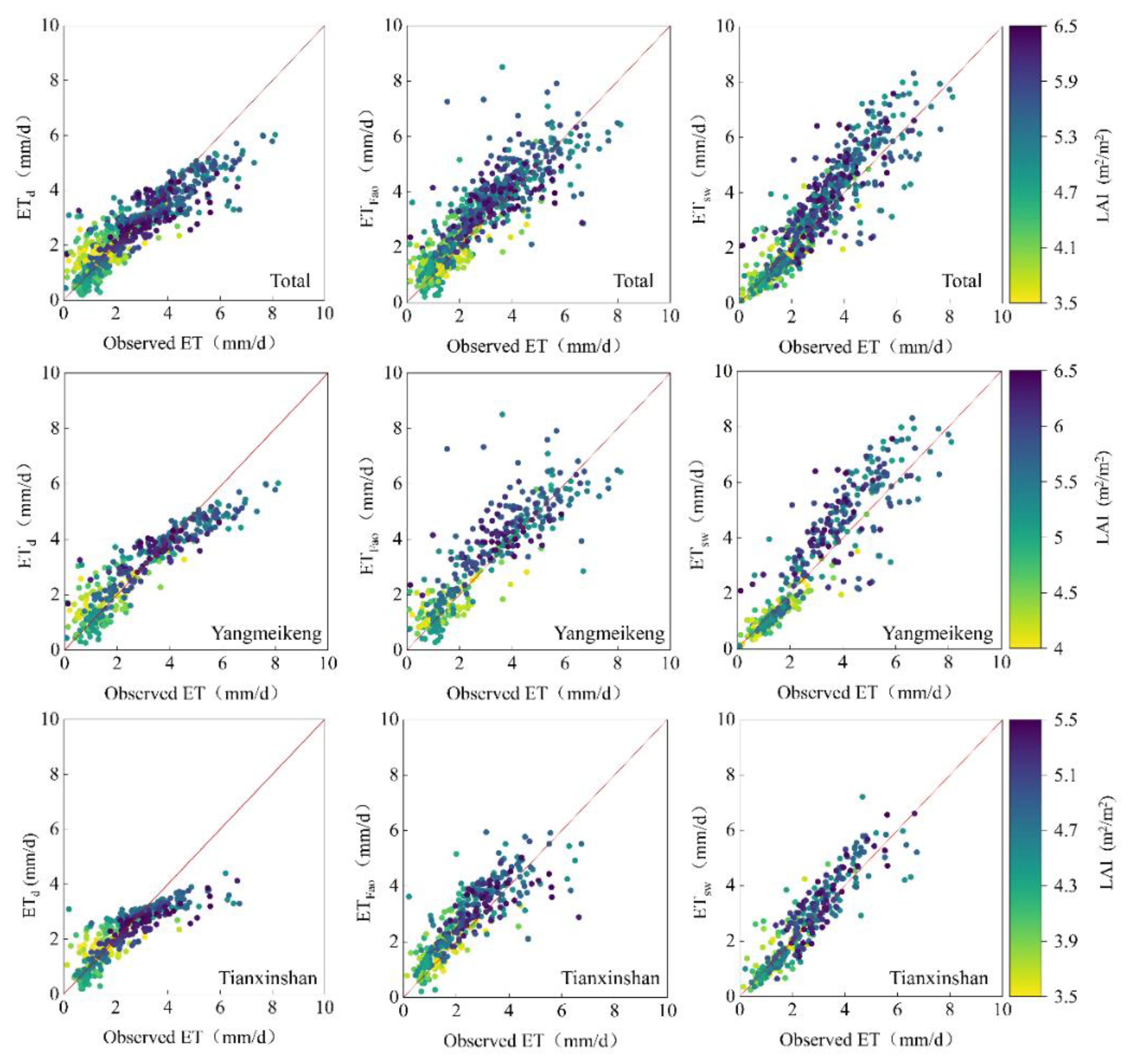
The flux footprint observed using the urban EC towers varied widely across different test days. Therefore, the simulation of urban ET should consider the impact of flux footprint on the measured ET. In addition, due to the higher LAI, the observed ET of the Yangmeikeng site was higher than that of the Tianxinshan site;

(2)

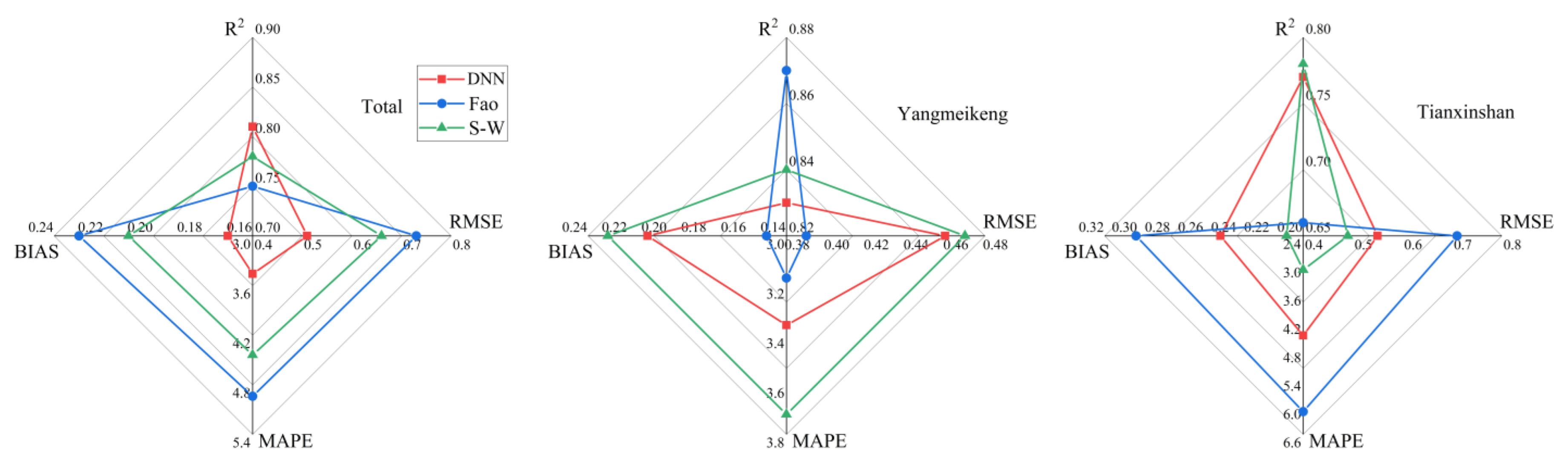
For the simulation of urban ET and T/ET at both main urban and suburban EC stations, the DNN model performed best, followed by the S-W model, and the FAO dual-K_c model. For the ET simulation, the R² and RMSE were 0.73 and 0.74 mm/day, 0.71 and 0.75 mm/day, and 0.69 and 0.81 mm/day for the DNN, S-W, and FAO dual-K_c models, respectively. For the T/ET simulation, the R² and RMSE were 0.81 and 0.17, 0.78 and 0.19, and 0.75 and 0.25 for the DNN, S-W, and FAO dual-K_c models, respectively;

(3)

For the three classic evapotranspiration models, T_a was the most important input variable and was extremely sensitive to the simulated urban ET. On the contrary, u was the least sensitive to simulating ET; hence, the u can be excluded from the input dataset in subsequent urban ET studies;

(4)

The error of the DNN model mainly comes from the simulation of extreme ET. The error of the S-W model lies in the determination of impedance parameters, and the uncertainty of the FAO dual-K_c model is the determination of vegetation coefficients;

(5)

When there is a large number and multiple types of meteorological, soil, and vegetation datasets available, the DNN model is recommended. When there are multiple types of meteorological, soil, and vegetation datasets available but the number of observation data is relatively smaller, the S-W model is recommended. When there are fewer types of input variables available, the FAO dual-K_c model is recommended to simulate urban ET and its components.

References

1. Bosch, J.M.; Hewlett, J.D. A review of catchment experiments to determine the effect of vegetation changes on water yield and evapotranspiration. J. Hydrol. 1982, 55, 3–23. [Google Scholar] [CrossRef]
2. Shukla, J.; Mintz, Y. Influence of land-surface evapotranspiration on the earth’s climate. Science 1982, 215, 1498–1501. [Google Scholar] [CrossRef] [PubMed]
3. Küçüktopcu, E.; Cemek, E.; Cemek, B.; Simsek, H. Hybrid Statistical and Machine Learning Methods for Daily Evapotranspiration Modeling. Sustainability 2023, 15, 5689. [Google Scholar] [CrossRef]
4. Sheng, H.P.; Fadzil, L.M.; Manickam, S.; Al-Shareeda, M.A. Vector Autoregression Model-Based Forecasting of Reference Evapotranspiration in Malaysia. Sustainability 2023, 15, 3675. [Google Scholar]
5. Sutanto, S.J.; Wenninger, J.; Coendersgerrits, A.; Uhlenbrook, S. Partitioning of evaporation into transpiration, soil evaporation and interception: A combination of hydrometric measurements and stable isotope analyses. Hydrol. Earth Syst. Sci. Discuss. 2012, 9, 3657–3690. [Google Scholar]
6. Qiu, G.Y.; Li, C.; Yan, C. Characteristics of soil evaporation, plant transpiration and water budget of Nitraria dune in the arid Northwest China. Agric. For. Meteorol. 2015, 203, 107–117. [Google Scholar] [CrossRef]
7. Hussain, S.; Mubeen, M.; Nasim, W.; Fahad, S.; Ali, M.; Ehsan, M.A.; Raza, A. Investigation of Irrigation Water Requirement and Evapotranspiration for Water Resource Management in Southern Punjab, Pakistan. Sustainability 2023, 15, 1768. [Google Scholar] [CrossRef]
8. Rai, P.; Kumar, P.; Al-Ansari, N.; Malik, A. Evaluation of Machine Learning versus Empirical Models for Monthly Reference Evapotranspiration Estimation in Uttar Pradesh and Uttarakhand States, India. Sustainability 2022, 14, 5771. [Google Scholar] [CrossRef]
9. Novotná, B.; Jurík, Ľ.; Čimo, J.; Palkovič, J.; Chvíla, B.; Kišš, V. Machine Learning for Pan Evaporation Modeling in Different Agroclimatic Zones of the Slovak Republic (Macro-Regions). Sustainability 2022, 14, 3475. [Google Scholar] [CrossRef]
10. Kuang, W. 70 years of urban expansion across China: Trajectory, pattern, and national policies. Sci. Bull. 2020, 65, 1970–1974. [Google Scholar] [CrossRef]
11. Tong, S.; Prior, J.; McGregor, G.; Shi, X.; Kinney, P. Urban heat: An increasing threat to global health. BMJ 2021, 375, n2467. [Google Scholar] [CrossRef] [PubMed]
12. Piroozfar, P.M.; Farr, E.; Pomponi, F. Urban heat island (uhi) mitigating strategies: A case-based comparative analysis. Sustain. Cities Soc. 2015, 19, 222–235. [Google Scholar]
13. Chen, H.; Jiang, A.Z.; Huang, J.J.; Li, H.; McBean, E.; Singh, V.; Zhang, J.; Lan, Z.; Gao, J.; Zhou, Z. An enhanced shuttleworth-wallace model for simulation of evapotranspiration and its components. Agric. For. Meteorol. 2022, 313, 108769. [Google Scholar] [CrossRef]
14. Chen, H.; Huang, J.J.; McBean, E.; Dash, S.S.; Li, H.; Zhang, J.; Lan, Z.; Gao, J.; Zhou, Z. Evapotranspiration partitioning based on field-stable oxygen isotope observations for an urban locust forest land. Ecohydrology 2022, 15, e2431. [Google Scholar] [CrossRef]
15. Kuang, W.; Zhang, S.; Li, X.; Lu, D. A 30 m resolution dataset of China’s urban impervious surface area and green space, 2000–2018. Earth Syst. Sci. Data 2021, 13, 63–82. [Google Scholar] [CrossRef]
16. Narita, K.I.; Nishikawa, T. Measurement of Sensible Heat Flux in an Urban Area by Eddy-Correlation Method. In Summaries of Technical Papers of Meeting Architectural Institute of Japan D; Architectural Institute of Japan: Tokyo, Japan, 1995. [Google Scholar]
17. Timmermans, W.J.; Kustas, W.P.; Anderson, M.C.; French, A.N. An intercomparison of the Surface Energy Balance Algorithm for Land (SEBAL) and the Two-Source Energy Balance (TSEB) modeling schemes. Remote Sens. Environ. 2007, 108, 369–384. [Google Scholar] [CrossRef]
18. Guzinski, R.; Anderson, M.C.; Kustas, W.P.; Nieto, H.; Sandholt, I. Using a thermal-based two source energy balance model with time-differencing to estimate surface energy fluxes with day–night MODIS observations. Hydrol. Earth Syst. Sci. 2013, 17, 2809–2825. [Google Scholar] [CrossRef] [Green Version]
19. Shuttleworth, W.J.; Wallace, J.S. Evaporation from sparse crops-an energy combination theory. Q. J. R. Meteorol. Soc. 1985, 111, 839–855. [Google Scholar] [CrossRef]
20. Evett, S.R.; Lascano, R.J. ENWATBAL.BAS: A mechanistic evapotranspiration model written in compiled basic. Agron. J. 1993, 85, 763–772. [Google Scholar] [CrossRef] [Green Version]
21. Kustas, W.P.; Norman, J.M. Evaluation of soil and vegetation heat flux predictions using a simple two-source model with radiometric temperatures for partial canopy cover. Agric. For. Meteorol. 1999, 94, 13–29. [Google Scholar] [CrossRef]
22. Sauer, T.; Norman, J.; Tanner, C.; Wilson, T. Measurement of heat and vapor transfer coefficients at the soil surface beneath a maize canopy using source plates. Agric. For. Meteorol. 1995, 75, 161–189. [Google Scholar] [CrossRef]
23. Wang, P.; Yamanaka, T.; Li, X.-Y.; Wei, Z. Partitioning evapotranspiration in a temperate grassland ecosystem: Numerical modeling with isotopic tracers. Agric. For. Meteorol. 2015, 208, 16–31. [Google Scholar] [CrossRef]
24. Wu, Y.; Du, T.; Ding, R.; Tong, L.; Li, S.; Wang, L. Multiple methods to partition evapotranspiration in a maize field. J. Hydrometeorol. 2017, 18, 139–149. [Google Scholar] [CrossRef] [Green Version]
25. Chen, H.; Huang, J.J.; McBean, E. Partitioning of daily evapotranspiration using a modified shuttleworth-wallace model, random forest and support vector regression, for a cabbage farmland. Agric. Water Manag. 2019, 228, 105923. [Google Scholar] [CrossRef]
26. Feng, Y.; Gong, D.; Mei, X.; Cui, N. Estimation of maize evapotranspiration using extreme learning machine and generalized regression neural network on the China Loess Plateau. Hydrol. Res. 2017, 48, 1156–1168. [Google Scholar] [CrossRef]
27. Patil, A.P.; Deka, P.C. An extreme learning machine approach for modeling evapotranspiration using extrinsic inputs. Comput. Electron. Agric. 2016, 121, 385–392. [Google Scholar] [CrossRef]
28. Zanetti, S.S.; Sousa, E.F.; Oliveira, V.P.S.; Almeida, F.T.; Bernardo, S. Estimating evapotranspiration using artificial neural network and minimum climatological data. J. Irrig. Drain. Eng. 2007, 133, 83–89. [Google Scholar] [CrossRef]
29. Nourani, V.; Paknezhad, N.J.; Tanaka, H. Prediction Interval Estimation Methods for Artificial Neural Network (ANN)-Based Modeling of the Hydro-Climatic Processes, a Review. Sustainability 2021, 13, 1633. [Google Scholar] [CrossRef]
30. Fan, J.; Yue, W.; Wu, L.; Zhang, F.; Cai, H.; Wang, X.; Lu, X.; Xiang, Y. Evaluation of SVM, ELM and four tree-based ensemble models for predicting daily reference evapotranspiration using limited meteorological data in different climates of China. Agric. For. Meteorol. 2018, 263, 225–241. [Google Scholar] [CrossRef]
31. Mehr, A.D.; Haghighi, A.T.; Jabarnejad, M.; Safari, M.J.S.; Nourani, V. A new evolutionary hybrid random forest model for SPEI forecasting. Water 2022, 14, 755. [Google Scholar] [CrossRef]
32. Yang, F.; White, M.; Michaelis, A.; Ichii, K.; Hashimoto, H.; Votava, P.; Zhu, A.-X.; Nemani, R. Prediction of continental-scale evapotranspiration by combining MODIS and ameriflux data through support vector machine. IEEE Trans. Geosci. Remote Sens. 2006, 44, 3452–3461. [Google Scholar] [CrossRef]
33. Allen, R.G. Crop evapotranspiration-guidelines for computing crop water requirements. FAO Irrig. Drain. Pap. (FAO) 1998, 56, D05109. [Google Scholar]
34. Er-Raki, S.; Chehbouni, A.; Guemouria, N.; Ezzahar, J.; Khabba, S.; Boulet, G.; Hanich, L. Citrus orchard evapotranspiration: Comparison between eddy covariance measurements and the FAO-56 approach estimates. Plant Biosyst. 2009, 143, 201–208. [Google Scholar] [CrossRef] [Green Version]
35. Chen, H.; Huang, J.J.; McBean, E.; Singh, V.P. Evaluation of alternative two-source remote sensing models in partitioning of land evapotranspiration. J. Hydrol. 2021, 597, 126029. [Google Scholar] [CrossRef]
36. Hu, X.; Shi, L.; Lin, G.; Lin, L. Comparison of physical-based, data-driven and hybrid modeling approaches for evapotranspiration estimation. J. Hydrol. 2021, 601, 126592. [Google Scholar] [CrossRef]
37. Jiang, S.Z.; Liang, C.; Zhao, L.; Gong, D.; Huang, Y.; Xing, L.; Zhu, S.; Feng, Y.; Guo, L.; Cui, N. Energy and evapotranspiration partitioning over a humid region orchard: Field measurements and partitioning model comparisons. J. Hydrol. 2022, 610, 127890. [Google Scholar] [CrossRef]
38. Mauder, M.; Foken, T.; Clement, R.; Elbers, J.; Kolle, O. Quality control of carboeurope flux data? part ii: Inter-comparison of eddy-covariance software. Biogeosci. Discuss. 2007, 4, 451–462. [Google Scholar]
39. Göckede, M.; Foken, T.; Aubinet, M.; Aurela, M.; Banza, J. Quality control of carboeurope flux data—Part 1: Coupling footprint analyses with flux data quality assessment to evaluate sites in forest ecosystems. Biogeosciences 2008, 5, 433–450. [Google Scholar] [CrossRef] [Green Version]
40. Davis, R.; Huntley, A.; Costa, D.; Worthy, G.; Castellini, M. Assessment of steady and non-steady state fuel homeostasis using the constant isotope infusion method. Minerva Radiol. Fisioter. E Radiobiol. 1987, 6, 28–37. [Google Scholar]
41. Yuan, Y.; Du, T.; Wang, H.; Wang, L. Novel Keeling-plot-based methods to estimate the isotopic composition of ambient water vapor. Hydrol. Earth Syst. Sci. 2020, 24, 4491–4501. [Google Scholar] [CrossRef]
42. Muoz-Sabater, J.; Dutra, E.; Agustí-Panareda, A.; Albergel, C.; Arduini, G.; Balsamo, G.; Boussetta, S.; Choulga, M.; Harrigan, S.; Hersbach, H.; et al. Era5-land: A state-of-the-art global reanalysis dataset for land applications. Earth Syst. Sci. Data 2021, 13, 4349–4383. [Google Scholar] [CrossRef]
43. LuisMerlin, O.-G.; SalahKhabba, O.-R.; Maria, S.E. Estimating the water budget components of irrigated crops: Combining the fao-56 dual crop coefficient with surface temperature and vegetation index data. Agric. Water Manag. 2018, 208, 120–131. [Google Scholar]
44. Paredes, P.; D’Agostino, D.; Assif, M.; Todorovic, M.; Pereira, L.S. Assessing potato transpiration, yield and water productivity under various water regimes and planting dates using the fao dual kc approach. Agric. Water Manag. 2018, 195, 11–24. [Google Scholar] [CrossRef]
45. Chiew, F.; Kamaladasa, N.N.; Malano, H.M.; McMahon, T.A. Penman-Monteith, FAO-24 reference crop evapotranspiration and class-A pan data in Australia. Agric. Water Manag. 1995, 28, 9–21. [Google Scholar] [CrossRef]
46. Sharma, G.; Singh, A.; Jain, S. A hybrid deep neural network approach to estimate reference evapotranspiration using limited climate data. Neural Comput. Appl. 2021, 33, 8017. [Google Scholar]
47. Atilla, Z.; Yamaç, S.S. Modelling of daily reference evapotranspiration using deep neural network in different climates. arXiv 2020, arXiv:2006.01760. [Google Scholar]
48. Pino-Vargas, E.; Taya-Acosta, E.; Ingol-Blanco, E.; Torres-Rúa, A. Deep Machine Learning for Forecasting Daily Potential Evapotranspiration in Arid Regions, Case: Atacama Desert Header. Agriculture 2022, 12, 1971. [Google Scholar] [CrossRef]
49. Lee, B.; Kim, N.; Kim, E.-S.; Jang, K.; Kang, M.; Lim, J.-H.; Cho, J.; Lee, Y. An artificial intelligence approach to predict gross primary productivity in the forests of South Korea using satellite remote sensing data. Forests 2020, 11, 1000. [Google Scholar] [CrossRef]
50. Jarvis, P.G. The interpretation of the variations in leaf water potential and stomatal conductance found in canopies in the field. Philos. Trans. R. Soc. Lond. B Biol. Sci. 1976, 273, 563–610. [Google Scholar] [CrossRef]
Figure 1. (a) Geographical location of the Shenzhen and Guangdong province; (b) Geographical location of the Yangmeikeng and Tianxinshan sites and photographs of the two EC towers.
Sustainability 15 09826 g001
Figure 2. Schematic diagram of the structure of three classic evapotranspiration models: (a) deep neural network (DNN) model; (b) Shuttleworth–Wallace model [13]; (c) FAO dual-kc model [33].
Sustainability 15 09826 g002
Figure 3. (a,b) Time series of wind speed and wind direction around the two EC stations in the year 2020; (cf) Time series of normalized in situ daily LAI, Ta, RH, and ET around the two EC stations in 2020 (YMK represents the Yangmeikeng station; TXS represents the Tianxinshan station).
Sustainability 15 09826 g003
Figure 4. Spatial distribution of 60%, 70%, 80%, and 90% flux footprint contours of two EC stations over the selected two test days.
Sustainability 15 09826 g004
Figure 5. Scatter plot of simulated ET using three classic evapotranspiration models and observed ET using EC system at the two EC stations (the colors of the scatter represent the different LAI conditions; ETd, ETfao, and ETsw represent the ET simulated using the DNN model, FAO dual-Kc model, and Shuttleworth–Wallace model, respectively).
Sustainability 15 09826 g005
Figure 6. Temporal series of simulated ET using three classic evapotranspiration models and observed ET using EC system at the two EC stations (a) Yangmeikeng site; (b) Tianxinshan site (ETd, ETfao, and ETsw represent the ET simulated using the DNN model, FAO dual-Kc model, and Shuttleworth–Wallace model, respectively).
Sustainability 15 09826 g006
Figure 7. Distributions of four statistical parameters for T/ET simulation using three classic evapotranspiration models at the two EC stations.
Sustainability 15 09826 g007
Figure 8. Relative importance of 6 input variables for urban ET simulation for the three classic evapotranspiration models.
Sustainability 15 09826 g008