Article

Gaining Profound Knowledge of Cholera Outbreak: The Significance of the Allee Effect on Bacterial Population Growth and Its Implications for Human-Environment Health

by
Gabriel Kolaye Guilsou
1,*,
Moulay-Ahmed Aziz-Alaoui
2,
Raymond Houé Ngouna
3,
Bernard Archimede
3 and
Samuel Bowong
4
1
Department of Mathematics and Computer Science, Faculty of Science, University of Maroua, Maroua P.O. Box 814, Cameroon
2
LMAH (Laboratoire de Mathématiques Appliquées du Havre), FR-CNRS-3335, ISCN (Institut des Systèmes Complexes en Normandie), Université de Normandie, 25 Rue Philippe Lebon, F-76600 Le Havre, France
3
LGP (Laboratoire Génie de Production), Toulouse INP/Ecole Nationale d’Ingénieurs de Tarbes, 47 Avenue d’Azereix, F-65000 Tarbes, France
4
Laboratory of Mathematics, Department of Mathematics and Computer Science, Faculty of Sciences, University of Douala, Douala P.O. Box 24157, Cameroon
*
Author to whom correspondence should be addressed.
Sustainability 2023, 15(13), 10384; https://doi.org/10.3390/su151310384
Submission received: 27 March 2023 / Revised: 11 June 2023 / Accepted: 23 June 2023 / Published: 30 June 2023

Abstract

:
Cholera is a bacterial disease that is commonly transmitted through contaminated water, leading to severe diarrhea and rapid dehydration that can prove fatal if left untreated. The complexity of the disease spread arises from the convergence of several distinct and interrelated factors, which previous research has often failed to consider. A significant scientific limitation of the existing literature is the simplistic assumption of linear or logistic dynamics of the disease spread, thereby impeding a thorough assessment of the effectiveness of control strategies. Since environmental factors are the most influential determinant of Vibrio bacterial growth in nature and are responsible for the resurgence, propagation, and disappearance of cholera epidemics, we have proposed a S-I-R-S model that combines bacterial dynamics with the Allee effect. This model takes into account the environmental influence and allows for a better understanding of the disease dynamics. Our results have revealed the phenomenon of bi-stability, with backward and forward bifurcation. Furthermore, our findings have demonstrated that the Allee effect provides a robust framework for characterizing fluctuations in bacterial populations and the onset of cholera outbreaks. This framework can be used for assessing the effectiveness of control strategies, including regular environmental sanitation programs, adherence to hygiene protocols, and monitoring of unfavorable weather conditions.

1. Introduction

Cholera, a bacterial waterborne disease caused by Vibrio cholerae [1], remains a major public health concern worldwide, particularly in low- and middle-income countries. The disease is primarily transmitted through contaminated water, via the fecal–oral route, or by the consumption of contaminated food, and can cause severe diarrhea and dehydration, leading to death if left untreated. Bacteria are typically transmitted among humans, and the characteristic pathology of the disease is caused by a toxin secreted by the bacteria, which targets receptors in the human intestine. Studies have estimated that every year, cholera results in 1.3 to 4.0 million cases and 21,000 to 143,000 deaths globally [1].
Understanding the dynamics of cholera transmission is crucial for developing effective prevention and control strategies. In addition to human factors (for instance, cultural habits that can negatively impact the quality of hygiene), environmental factors such as water quality, temperature, rainfall, and nutrient availability also play a critical role in the disease spread [2]. Some decades ago, temperature and nutrient availability have been shown to affect the growth and survival of V. cholerae in water, while changes in rainfall can lead to contaminated water sources [3].
In a prior study [4], we suggested a mathematical model of cholera that examines the effects of environmental factors on the dynamic transmission of the disease within a human community. However, the proposed model comprised nine state variables, with four specifically representing the bacterial population. A research question therefore arises upon completing the previous work: what should be the realistic formulation of a cholera model that considers the effects of environmental factors and can contribute to improving the understanding and defining efficient control strategies of the epidemic? In this article, we develop a simplified version that preserves the environmental factors while incorporating the Allee effect into the dynamics of the bacteria. This modification will enhance our understanding of the complex relationship between human and environmental factors in cholera transmission and can assist in the formulation of more effective prevention and control strategies. The main objective of this research is to comprehensively explore the dynamics of cholera outbreaks, specifically through the analysis of the Allee effect and its integration into a robust mathematical model. Such an approach provides compelling evidence supporting the existence and stability of disease equilibria.
The present research work focuses on the epidemiological dynamics of cholera outbreaks by analyzing the interplay between the human host and bacterial population through a mathematical modelling framework. In particular, the study conducted delves into the dynamical behavior of both populations and their interdependence, utilizing a mathematical epidemiology approach. A common epidemiological S-I-R model, used to study the spread of infectious diseases in a population, divides this population into three compartments: susceptible ( S ) , infected ( I ) , and recovered ( R ) individuals. Such a model assumes that individuals move between compartments based on certain rates. In this study, we made the assumption that recovered individuals can become susceptible again, which aligns with the definition of a S-I-R-S model. Furthermore, we incorporated the Allee effect on bacterial population (B) growth to gain profound knowledge and understanding of the disease spread and the interrelationship between human and environmental health.
The present research work calls for a one-health approach and aims to provide a comprehensive analysis of the study results and their implications for developing strategies to prevent and control cholera, taking into account the interplay between human health and environmental health.
The rest of the paper is organized as follows: In Section 2, the materials and methods of the scientific proposal are presented, including a brief summary of the related work, and the description of the modelling approach. Section 3 presents the results of the research conducted, in terms of mathematical modelling of the dynamics of cholera, while Section 4 provides discussion on numerical simulations of few scenarios. The concluding section summarises the scientific proposal and highlights potential avenues for future research aimed at expanding upon the current findings.

2. Materials and Methods

This research is rooted in mathematical epidemiology and utilizes simulations to offer valuable insights into the key findings. In this section, the main results of the research conducted, in terms of mathematical modelling of the cholera dynamics with the Allee effect, are described and then discussed, through sensitivity analysis and simulations. To highlight the fundamental of the modelling approach, a brief summary of the related work is first presented.

2.1. Related Work

For a chronological history of the modelling of cholera, we refer the reader to the works [5,6] which represent the earliest mathematical models of cholera. We also proposed a mathematical model of cholera in a periodic environment with public health worker interventions such as sanitation or campaign awareness. In this study, we combined the bacteria model that we developed and studied in [7] with a S-I-R-S human cholera model in [8]. The findings showed that the control cholera should consider both sensitization and sanitation with a strong focus on sanitation.
Most of the current models in the literature assume that bacterial growth follows a linear or logistic dynamic. This assumption has the advantage of simplifying some of the mathematical analyses and making it easier to apply well-known theories in dynamical systems. However, the current information on the V. cholerae bacteria necessitates a review of its mathematical dynamics in the environment. It has been discovered that environmental aquatic bacteria, including V. cholerae O1 and V. cholerae non-O1, have the ability to survive the stress caused by environmental factors such as temperature, pH, and lack of nutritional resources [9]. To adapt to these conditions, the bacteria undergo metabolic changes that allow them to survive the environmental stress, similar to a phenomenon of dormancy. These cells are considered “viable but non-culturable” (VNC) because their ability to be cultivated on bacteriological culture media is lost [10]. This dormant state is considered a survival strategy in the natural environment for many species of bacteria [9].
The return to a cultivable state is possible when environmental factors causing stress become favorable for the development and growth of the bacterial population. This metabolic change necessitates reconsideration of the survival of pathogenic bacteria in the environment and its dynamics in the aquatic ecosystem. This metabolic change is also considered a possible hypothesis for the “disappearance” of V. cholerae in aquatic ecosystems during colder months. These field observations therefore highlight the limitations of some current mathematical cholera models in handling the full dynamics of the disease studied, and indicate that mathematical models of cholera must consider these environmental factors that are responsible for the resurgence and propagation of this epidemic.
The mathematical model of cholera proposed in [4] examines the effects of environmental factors on the dynamic transmission of the disease within a human community. This model accounts for the virulence of the bacteria and the commensalism relationship between the bacteria and their aquatic reservoirs. The findings showed that the aquatic reservoirs play a significant role in explaining the endemicity of the disease. However, the proposed model included several state variables (nine in total), with four representing the bacteria population. We suggest simplifying it, retaining the environmental factors while incorporating the Allee effect on the bacteria dynamics. The model construction, including its main principles, is presented in the next subsection.

2.2. Model Construction

In the context of bacterial population dynamics, unfavorable environmental conditions can limit the maximum population size, denoted θ . This value represents a critical concentration below which the population will go extinct, and above which the population will grow to a saturation value, denoted ρ . This type of dynamic is known as the “Allee Effect”. The Allee Effect is a biological phenomenon, named after W. C. Allee, that describes a positive relationship between population density and per capita growth rate of a species. In the presence of the Allee Effect, the population growth rate decreases at low population densities. Species under the Allee Effect do not thrive at low population densities, but the effect typically saturates or disappears as populations grow larger.
Since environmental factors greatly influence the growth of Vibrio bacteria in nature, and are responsible for the resurgence, propagation, and disappearance of cholera epidemics, we proposed a mathematical model that combines a bacterial dynamics with Allee effect and a S-I-R-S model to account for these environmental factors. Sensitivity analysis of the proposed model is conducted to determine the degree of influence of each parameter. Additionally, the different disease-free equilibrium (DFE) points of the system are computed, and their local stability conditions and attraction domains are determined. We also analyzed the basic reproduction number R 0 0 and R 0 ( Q ρ ) of the DFE Q 0 and Q ρ respectively. This allowed us to infer that the phenomena of backward bifurcation and forward bifurcation could be realized at R 0 0 = 1 in the neighborhood of Q 0 . However in a neighborhood of Q ρ , only forward bifurcation is realized at R 0 0 = 1 .
We classify individuals in a population of interest according to their disease status, distinguishing between susceptible individuals ( S ) , infected individuals ( I ) , and recovered individuals ( R ) . Once infected, individuals can recover from the disease at rate α . As suggested in many studies [11,12], recovered individuals may only have partial immunity. Then, recovered individuals can lose their immunity and return to the susceptible stage at rate γ . The parameters μ and d are introduced to represent the natural human mortality and cholera induced death rate of infected individuals, respectively. Infected individuals contribute to the concentration of Vibrios at rate δ .
For the population of bacteria, denoted B, we assume that their reproduction with the Allee effect includes the limitation of resources and the natural mortality is therefore:
f ( B ) = r B ( B θ ) ( ρ B ) , = r B 3 + r ( ρ + θ ) B 2 r ρ θ B ,
where r ( ρ + θ ) B 2 is the reproduction of bacteria, the term r B 3 is the intra-specific competition due to limited resource, and the term r ρ θ B is the mortality of bacteria.
Therefore, drawing upon these hypotheses, the dynamics of cholera epidemics proposed to address the research question can be described by the following system of non-autonomous differential equations with the Allee effect:
S ˙ = Λ ( λ + μ ) S + γ R , I ˙ = λ S ( μ + d + α ) I , R ˙ = α I ( μ + γ ) R , B ˙ = r B ( B θ ) ( ρ B ) + δ I ,
where 0 < θ < ρ and the force of infection of the model suggested is defined by:
λ = β B K + B .
The structure of the proposed model is depicted in Figure 1. The dashed arrow from I to B indicates contamination of the environment by humans and the second dashed arrow indicates influence of contaminated environment on infection force.
In the following, we consider ω = μ + d + α , and define the values used for numerical simulation in Table 1. To evaluate the robustness of the proposed model, a sensitivity analysis was conducted, as elaborated in the following section.

3. Results

The main results presented in this section are concerned with (i) the sensitivity analysis of proposed model (2), (ii) the proof of the basic properties, (iii) the existence and stability of the model equilibria, and (iv) a few simulations of the model using parameters of Table 1. Three of these parameters are found in the literature and the others were assumed (chosen arbitrarily, yet within admissible boundaries). This is highlighted in column “source” of Table 1.

3.1. Sensitivity Analysis

The aim of the sensitivity analysis was to determine the robustness of the model to changes in parameter values, which can help identify the most influential parameters in the disease dynamics [16]. A Latin Hypercube Sampling (LHS) scheme [17,18] was utilized to sample 1000 values for each input parameter. The sampling was conducted using a uniform distribution over a range of biologically realistic values. It should be noted that the parameters of Table 1 were used as central values of the uniform distribution sampling performed.
Using model (2) with a time period of 7000 days, 1000 model simulations were performed by randomly pairing sampled values for all LHS parameters. Then, four outcome measures were calculated for each run: the maximum and total size (cumulative effective) of state variables S, I, R, and B over the model’s time span, Partial Rank Correlation Coefficients (PRCC), and corresponding p-values.
The decision rule for the sensitivity analysis is the following: an output is assumed sensitive to an input if the corresponding PRCC is less than 0.50 or greater than + 0.50 , and the corresponding p-value is less than 0.05 .
The results are presented in Table 2 where each row displays the value of a parameter against its corresponding variable: positive PRCC value indicates a parameter whose increase causes an increase in the corresponding output variable, while on the contrary, negative PRCC value indicates a parameter whose increase leads to a decrease in the corresponding output variable.
According to these results:
  • the parameters Λ , β , δ , θ , and ρ should significantly affect at least one state variable of model (2);
  • Λ is not related to transmission of disease;
  • influence of β suggests to sensitize population to avoid getting in touch with bacteria;
  • influences of θ and ρ suggest to intensify sanitation campaigns by destroying reservoirs of V. cholera.
To sustain these results, the mathematical validity of the proposed model is analyzed in the next section.
Table 2. Table of PRCC parameters with the variables of the model.
PRCCs and Significance
ParametersRange S I R B
Λ [1–300]0.8970 **0.0968 *0.0171−0.0332
β [10 6 –0.999]−0.9580 *−0.2359 **0.1221 **−0.1702 **
δ [1–1000]−0.8934 **−0.05450.0885−0.1173 *
μ [10 6 –0.999]−0.0718−0.02550.0270−0.0818
d[10 6 –0.999]0.02900.0432−0.0676−0.0462
r[10 6 –0.999]−0.0282−0.01800.03950.0291
γ [10 6 –0.999]−0.03880.01470.0577−0.0106
α [10 6 –0.999]0.10100.06800.05300.0948
K[10 4 –10 17 ]0.00500.03350.0092−0.0213
ρ [10 5 –10 20 ]−0.0723−0.1149 *0.05610.6220 **
θ [10 3 –10 15 ]0.02100.06280.04730.5029 *
*: p-value < 0.01, **: p-value < 0.001.

3.2. Basic Properties

In this section, we examine the basic properties of the solutions of the proposed model, namely their positivity, boundedness, and positive invariance of sets used in studying the dynamical system. These properties are crucial in demonstrating the mathematical and epidemiological coherence of model (2), as well as in establishing the stability of the results.

3.2.1. Positivity and Boundedness of Solutions

Obviously, model (2) which is a C differential system, admits a unique maximal solution for any associated Cauchy problem.
Theorem 1. 
The region Ω defined by:
Ω = Ω H × Ω B ,
where
Ω H = ( S , I , R ) + 3 , 0 N Λ μ a n d Ω B = B + , 0 B r ρ 2 μ ( ρ θ ) + δ Λ r ρ μ ( ρ θ ) ,
is positively invariant and attracting for model (2).
Proof. 
The proof is provided in two steps.
Step 1. 
We show that for any initial condition ( t 0 = 0 , X 0 = ( S ( 0 ) , I ( 0 ) , R ( 0 ) , B ( 0 ) ) ( R + * ) 4 ) , the maximal solution ( [ 0 , T [ , X = ( S ( t ) , I ( t ) , R ( t ) , B ( t ) ) ) of the Cauchy problem associated with system (2) is non-negative.
Let T ˜ = sup t ˜ [ 0 ; T [ , ( S ( t ) , I ( t ) , R ( t ) , B ( t ) ) ( R + * ) 4 and let us show that T ˜ = T .
Suppose that T ˜ < T . At least one of the following conditions is satisfied: S ( T ˜ ) = 0 , I ( T ˜ ) = 0 , R ( T ˜ ) = 0 , or B ( T ˜ ) = 0 .
Suppose S ( T ˜ ) = 0 . Then from the first equation of model (2),
d d t S e 0 t λ ( r ) + μ d r = ( Λ + γ R ) e 0 t λ ( r ) + μ d r , t [ 0 ; T ˜ [ .
This implies that
d d t S e 0 t λ ( r ) + μ d r > 0 , t [ 0 ; T ˜ [ .
Integrating Equation (6) from 0 to T ˜ yields:
S ( T ˜ ) S ( 0 ) e 0 T ˜ λ ( r ) + μ d r > 0 .
Similarly, one can show that I ( T ˜ ) > 0 , R ( T ˜ ) > 0 , and B ( T ˜ ) > 0 , which is contradictory. Therefore, T ˜ = T and consequently, the maximal solution ( S ( t ) , I ( t ) , R ( t ) , B ( t ) ) of the Cauchy problem associated to model (2) is non-negative.
Step 2. 
We then prove that the total population of humans and bacteria satisfies the boundedness property. We first split model (2) into two parts, the human population (i.e., S ( t ) , I ( t ) and R ( t ) ) and the pathogen population (i.e., B ( t ) ).
Let N = S + I + R . Using the equation of model (2), one can deduce that
N ˙ = Λ μ N d I Λ μ N .
Thus,
0 N ( t ) Λ μ + N ( 0 ) Λ μ e μ t ,
where N ( 0 ) represents the initial value of N ( t ) .
The lower limit comes naturally from the fact that the model variables are non-negative ( t [ 0 , T [ ) since they monitor human populations.
Thus, 0 N ( t ) Λ μ whenever 0 N ( 0 ) Λ μ .
Suppose 0 N ( 0 ) Λ μ . From the last equation of model (2) and using the fact that I ( t ) Λ / μ for all t 0 , one has:
B ˙ f ( B ) + δ Λ μ ,
where f ( B ) = r B ( B θ ) ( ρ B ) .
Note that lim B + f ( B ) = and f ( B ) is a decreasing in [ ρ ; + [. The equation of the tangent of f ( B ) at B = ρ is given by y ( B ) = r ρ ( ρ θ ) B + r ρ 2 ( ρ θ ) .
It follows that, for B > ρ , we have:
B ˙ r ρ 2 ( ρ θ ) + δ Λ μ r ρ ( ρ θ ) B .
Integrating the above differential inequality yields:
0 B ( t ) r ρ 2 μ ( ρ θ ) + δ Λ r ρ μ ( ρ θ ) + B ( 0 ) r ρ 2 μ ( ρ θ ) + δ Λ r ρ μ ( ρ θ ) e r ρ ( ρ θ ) t ,
where B ( 0 ) is the initial condition of B ( t ) .
Thus, as t + ,
B ( t ) r ρ 2 μ ( ρ θ ) + δ Λ r ρ μ ( ρ θ ) .
Since each maximal solution of the Cauchy problem associated to model (2) is positive and bounded, each solution is global.
Combining Step 1 and Step 2, Theorem 1 can be derived from the classical theory of dynamical systems. This completes the proof. □
In conclusion, the proposed model (2) is mathematically and epidemiologically well-posed, thereby making it adequate to study the dynamics of the flow generated in Ω .

3.2.2. Positively Invariant Sets

We present here some results that will be useful for studying the dynamical system modeled in (2), based on two Lemmas which are described and subsequently proved below.
To undertake a comprehensive analysis of the dynamical system defined in (2), we introduce essential sets that are positively invariant, and offer valuable insights into the behavior of the system.
Let ϵ ] 0 ; θ [ and B m = r ρ 2 μ ( ρ θ ) + δ Λ r ρ μ ( ρ θ ) .
One denotes:
Ω 0 = { ( S , I , R , B ) Ω : 0 < B < θ ϵ } , Ω θ ϵ = { ( S , I , R , B ) Ω : θ ϵ < B < B m } ,
Ω θ = ( S , I , R , B ) Ω : θ B ( t ) B m and Ω ρ = ( S , I , R , B ) Ω : ρ B ( t ) B m .
Lemma 1. 
The sets Ω θ and Ω ρ are positively invariant for model (2).
Proof. 
To prove Lemma 1, we simply consider the fact that B ˙ δ I 0 for all value of B [ θ ; ρ ] . This means that every trajectory of B starting in [ θ ; ρ ] will grow and cross the value ρ , and then remain in [ ρ ; B m ] . It would be maintained on the value ρ if I = 0 . □
Lemma 2. 
The set Ω ρ is a compact attractor for model (2).
Proof. 
The proof of Lemma 2 is essentially based on the fact that Ω ρ is an invariant set and also on the fact that for every solution X ( t ) of model (2) associated to the initial condition X ( 0 ) = ( S ( 0 ) , I ( 0 ) , R ( 0 ) , B ( 0 ) ) Ω θ , we have lim t + d i s t ( X ( t ) , Ω ρ ) = 0 .
Thus, Ω ρ is an attractor and his attraction domain contains Ω θ . □

3.3. Existence and Stability of Equilibria

The existence and stability of equilibria in epidemiological models are important properties that allow us to make robust predictions about the spread of infectious diseases in a population. By understanding these properties, we can develop effective strategies for controlling and preventing the spread of diseases.

3.3.1. Existence of Disease-Free Equilibria

The proposed model has three disease-free equilibria obtained by setting the right side of the equations in (2) to zero with I = 0 .
Q 0 = S 0 , 0 , 0 , 0 , Q θ = S θ , 0 , 0 , θ , and Q ρ = S ρ , 0 , 0 , ρ ,
where
S 0 = Λ μ , S θ = Λ ( θ + K ) β θ + μ ( θ + K ) , and S ρ = Λ ( ρ + K ) β ρ + μ ( ρ + K ) .

3.3.2. Stability of Equilibria and Threshold Quantities

The local stability of the DFEs of model (2) is summarized in the following Proposition.
Proposition 1. 
L e t R 0 0 = β Λ δ K r ρ θ μ ( μ + d + α ) ,
and
R 0 ρ = β μ ( ρ + K ) + β ρ ( μ + d + α ) α ρ γ μ + γ + K Λ δ ( K + ρ ) r ρ ( ρ θ ) .
For the dynamical system (2),
(i) 
If R 0 0 < 1 , the DFE Q 0 is locally stable.
(ii) 
If R 0 ρ < 1 , the DFE Q ρ is locally stable.
(iii) 
The DFE Q θ is always unstable.
To prove Proposition 1, we will use Lemma 3 proposed by Kamgang J.C. and Sallet [19].
Lemma 3. 
Let M be a square Metzler matrix written in block form M = A B C D where A and D are square matrices. Then, matrix M is Metzler stable if and only if matrices A and D C A 1 B (or D and A B D 1 C ) are Metzler stable.
Proof. 
Let Q x = ( S x , 0 , 0 , B x ) any DFE. The Jacobian of model (2) at the point Q x is denoted by the following matrix J ( Q x ) :
J ( Q x ) = μ β B x B x + K 0 γ β S x K ( K + B x ) 2 β B x B x + K ω 0 β S x K ( K + B x ) 2 0 α ( μ + γ ) 0 0 δ 0 L x ,
where L x = r θ ρ 2 r ( θ + ρ ) B x + 3 r B x 2 and ω = μ + d + α .
Matrix J ( Q x ) can be expressed in the form of the matrix M in Lemma 3, with:
A = μ β B x B x + K 0 β B x B x + K ω , B = γ β S x K ( K + B x ) 2 0 β S x K ( K + B x ) 2 , C = 0 α 0 δ ,
and D = ( μ + γ ) 0 0 L x .
Obviously, matrix A is a Metzler stable matrix. A simple calculation gives:
( D C A 1 B ) | Q x = Q 0 = ( μ + γ ) β S 0 α K ω 0 r θ ρ + β S 0 δ K ω ,
( D C A 1 B ) | Q x = Q ρ = ( μ + γ ) + α γ β ρ ω [ β ρ + μ ( ρ + K ) ] β S ρ K α μ ( K + ρ ) ω [ β ρ + μ ( ρ + K ) ] δ γ β ρ ω [ β ρ + μ ( ρ + K ) ] r ( ρ θ ) ρ + β S ρ K δ μ ( K + ρ ) ω [ β ρ + μ ( ρ + K ) ] ,
and
( D C A 1 B ) | Q x = Q θ = ( μ + γ ) + α γ β θ ω [ β θ + μ ( θ + K ) ] β S θ K α μ ( K + θ ) ω [ β θ + μ ( θ + K ) ] δ γ β θ ω [ β θ + μ ( θ + K ) ] r ( ρ θ ) θ + β S θ K δ μ ( K + θ ) ω [ β θ + μ ( θ + K ) ] .
Thus, matrix ( D C A 1 B ) | Q x = Q 0 is stable if and only if:
t r ( ( D C A 1 B ) | Q x = Q 0 ) < 0 β S 0 δ K ω [ r θ ρ + μ + γ ] < 1 D e t ( ( D C A 1 B ) | Q x = Q 0 ) > 0 β S 0 δ K ω r θ ρ < 1 .
so that ( D C A 1 B ) | Q x = Q 0 is a Metzler stable matrix when:
R 0 0 = β S 0 δ K r θ ρ ( μ + d + α ) < 1 .
Similarly, we can easily prove that matrix ( D C A 1 B ) | Q x = Q ρ is a Metzler stable matrix if:
R 0 ρ = β μ ( ρ + K ) + β ρ ( μ + d + α ) α ρ γ μ + γ + K Λ δ ( K + ρ ) r ρ ( ρ θ ) < 1 .
For the matrix ( D C A 1 B ) | Q x = Q θ , the condition d e t ( ( D C A 1 B ) | Q x = Q θ ) > 0 gives:
( μ + γ ) [ β θ + μ ( θ + K ) ] α γ β θ + S θ K δ ( μ + γ ) μ ( θ + K ) r ρ ( ρ θ ) α γ θ < 1 .
Also, the condition t r ( ( D C A 1 B ) | Q x = Q θ ) < 0 gives:
α γ β θ ( μ + γ ) [ β θ + μ ( θ + K ) ] + r θ ( ρ θ ) μ + γ + β S θ K δ μ ( K + θ ) ω [ β θ + μ ( θ + K ) ] < 1 .
This contradicts the condition d e t ( ( D C A 1 B ) | Q x = Q θ ) > 0 .
This concludes the proof. □
We are now interested in global and asymptotic stability of the disease- and bacteria-free equilibrium point Q 0 .
Following Kamgang and Sallet [19], model (2) can be written in the following form:
x ˙ s = A 1 ( x ) ( x s x s 0 ) + A 12 ( x ) x i , x ˙ i = A 2 x i ,
where x s = ( S , R ) T represents susceptible and recovered individuals, x i = ( I , B ) T represents the infectious individuals and the population of bacteria. x s 0 = ( S 0 , 0 ) is the non-zero component of the DFE, x = ( x s , x i ) T ,
A 1 ( x ) = ( μ + λ ) γ 0 ( γ + μ ) ,   A 12 ( x ) = 0 β S 0 B + K α 0 ,   and A 2 ( x ) = ω β S B + K δ r ( B θ ) ( ρ B ) .
The conditions described below, H 1 , , H 5 , should be satisfied to guarantee the global asymptotic stability (GAS) of Q 0 .
Hypothesis 1 
( H 1 ). Model (17) is defined on a positively invariant set D of the non-negative orthant, and is dissipative on D .
Hypothesis 2 
( H 2 ). The sub-system x ˙ s = A 1 ( x s , 0 ) ( x s x s 0 ) is globally asymptotically stable at the equilibrium x s 0 on the canonical projection of D on R + 2 .
Hypothesis 3 
( H 3 ). Matrix A 2 ( x ) is Metzler (a Metzler matrix is a matrix with non-negative off-diagonal entries) and is irreducible for any given x D .
Hypothesis 4 
( H 4 ). There exists an upper-bound matrix A 2 ¯ for M = A 2 ( x ) | x D with the property that either A 2 ¯ M or, if A 2 ¯ M , then for any x D such that A 2 ¯ = A 2 ( x ) , x R + 2 × 0 .
Hypothesis 5 
( H 5 ). ρ ( A 2 ¯ ) < 0 is satisfied, where ρ ( A 2 ¯ ) < 0 denotes the largest real part of the eigenvalues of A 2 ¯ .
If conditions H 1 , , H 5 are satisfied, then Q 0 is globally asymptotically stable in D .
The result of the Kamgang–Sallet approach [19] uses the algebraic structure of model (17), namely the fact that A 1 ( x ) and A 2 ( x ) are Metzler matrices. Since in the said approach the matrix A 2 ( x ) is required to be irreducible, we further restrict the domain of the system to:
D = x s , x i Ω , x s 0 .
The set D is positively invariant because only the initial point of any trajectory can have x s = 0 . Therefore, we restrict the domain of model (17) to D , where A 2 ( x ) irreducible.
Therefore,
A 2 ( x ) is   Metzler   and   irreducible   for   all x D .
The sub-system x ˙ s = A 1 ( x s , 0 ) ( x s x s 0 ) is equivalent to:
S ˙ = Λ + γ R μ S , R ˙ = ( δ + μ ) R .
Resolving the above equations and taking the limit of solutions when t goes to infinity yields:
lim t + S ( t ) = Λ μ and lim t + R ( t ) = 0 .
Therefore, x s 0 = ( S 0 , 0 ) is a globally asymptotically stable equilibrium of the reduced system (18) on the sub-domain D . Then, the hypothesis H 2 is satisfied.
Let ϵ ] 0 ; θ [ , since max B [ 0 ; θ ϵ ] r ( B θ ) ( ρ B ) = r ϵ ( ρ θ ) r ϵ 2 we have the following upper-bound matrix of A 2 ( x ) in Ω 0 Ω :
A 2 ¯ = ω β S 0 K δ r ϵ ( ρ θ ) r ϵ 2 .
Using Kamgang and Sallet’s result [20], the sub-matrix A 2 ¯ is a Metzler stable matrix if:
R 0 0 ξ ,
where
ξ = 1 θ ρ ϵ ( ρ θ ) θ ρ < 1 .
We can now apply Theorem 4.3 in Kamgang and Sallet [20] and conclude that under the condition (19) the DFE ( x s 0 ; 0 ) of model (2) is globally asymptotically stable in Ω 0 . We have established the following result for the global stability of the DFE Q 0 .
Theorem 2. 
Let ϵ ] 0 ; θ [ , if R 0 0 < ξ < 1 then the DFE point Q 0 of model (2) is globally asymptotically stable in the domain Ω 0 and unstable if R 0 0 > 1 . However, when ξ < R 0 0 < 1 the backward bifurcation phenomenon may occur in Ω 0 , i.e., the DFE Q 0 , may coexist with two endemic equilibria, one asymptotically stable and one unstable.
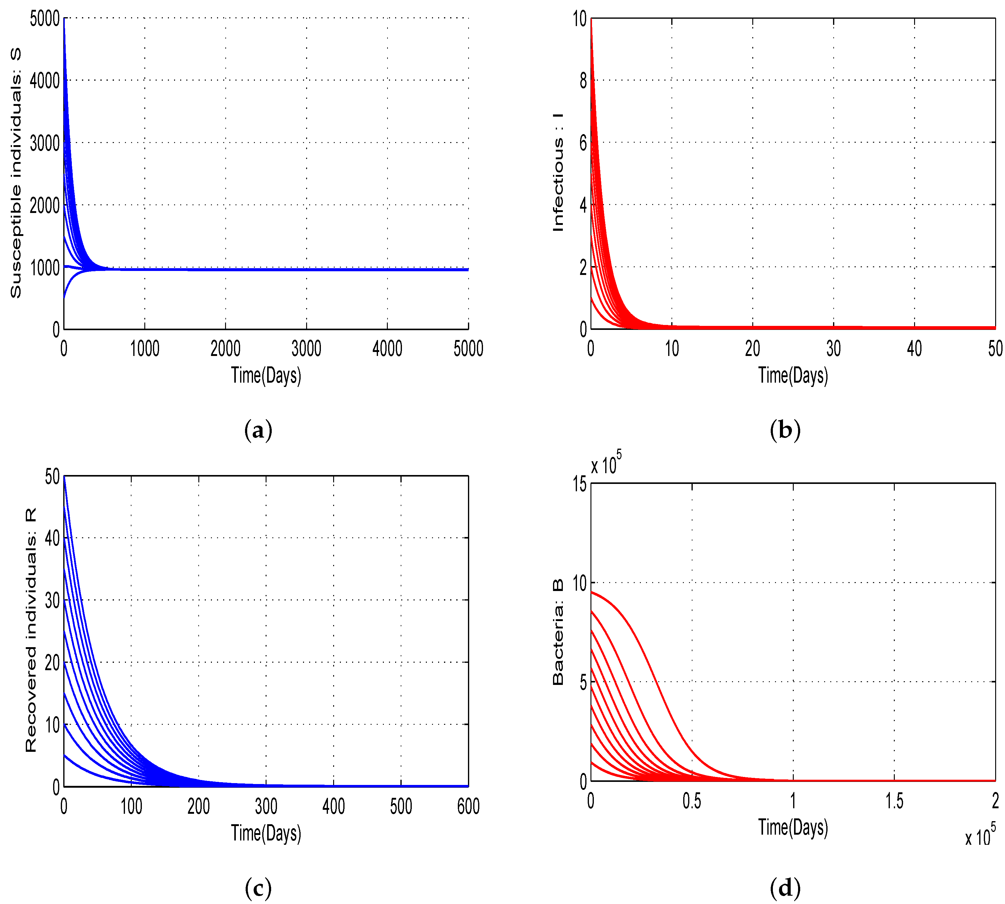
Figure 2 is an illustration of Theorem 2, showing the stability of the DFE of model (2) when initial conditions are taken in the basin of attraction of Q 0 and R 0 0 < ξ < 1 . So, when Λ = 10 , β = 0.0001 , ϵ = 50 , 000 (so that θ ϵ = 9.5 × 10 5 ) and the remaining parameters are consistent with those listed in Table 1, we have R 0 0 = 0.0103 and ξ = 0.0495 . Under these conditions, when various initial conditions are chosen in attraction domain of Q 0 , it is seen in Figure 2 that the disease disappears.
The backward bifurcation phenomenon is illustrated by Figure 3 where time series of model are presented (2) when Λ = 50 , β = 0.0015 , θ = 10 6 (so that θ ϵ = 9.5 × 10 5 ) and ϵ = 50 , 000 (so R 0 0 = 0.7702 and ξ = 0.0495 ). It clearly appears that ξ R 0 0 < 1 .
The epidemiological significance of the phenomenon of backward bifurcation is that the classical requirement of ξ R 0 0 < 1 is, although necessary, no longer sufficient for disease eradication when initial conditions are taken in attraction domain of Q 0 . In such a scenario, disease elimination would depend of various initial sizes of the population (state variables) chosen Ω 0 . That is, the presence of backward bifurcation in the cholera transmission (2) suggests that the feasibility of controlling a cholera epidemic when ξ R 0 0 < 1 is always dependent on the initial sizes of the population even if they are chosen in Ω 0 . To illustrate this situation, model (2) was simulated for various initial conditions ( S ( 0 ) , I ( 0 ) , R ( 0 ) , B ( 0 ) ) taken firstly in the domain D 1 = ] 0 ; 50 , 000 ] × ] 0 ; 10 ] × ] 0 ; 50 ] × 2 × 10 5 , 3 × 10 5 , 4 × 10 5 , 5 × 10 5 and secondly for various initial conditions ( S ( 0 ) , I ( 0 ) , R ( 0 ) , B ( 0 ) ) taken in the domain D 2 = ] 0 ; 50 , 000 ] × ] 0 ; 10 ] × ] 0 ; 50 ] × 7.5 × 10 5 , 8 × 10 5 , 9 × 10 5 , 9.5 × 10 5 . As is presented in Figure 3, the cholera epidemic disappears in the first case while in the second case disease and bacteria persist in the environment.
In order to derive an expression for the region of stability of the boundary equilibrium Q ρ we measure the capacity of infectious to invade and persist in a human population at the in the neighborhood of Q ρ . Applying the methods in van den Driessche and Watmough at equilibrium Q ρ [21], we find the basic reproduction number of infectious in a population model (2) is (see Appendix A for details):
R 0 ( Q ρ ) = β Λ K δ [ β ρ + μ ( ρ + K ) ] ( K + ρ ) ω r ρ ( ρ θ ) .
This formalism permits the derivation of a threshold condition for endemicity of cholera epidemic in population where model (2) is at equilibrium Q ρ .
Proposition 2 expresses this result in terms of stability for equilibrium point Q ρ .
Proposition 2. 
The equilibrium point Q ρ of model (2) is stable if R 0 ( Q ρ ) < 1 and unstable if R 0 ( Q ρ ) > 1 .
The following Proposition gives relationship between stability of Q 0 and of Q ρ .
Proposition 3. 
Let 0 < ϵ < θ , if R 0 0 < ξ then R 0 ( Q ρ ) < 1 .
Proof. 
Let 0 < ϵ < θ ,
R 0 0 < ξ R 0 0 < ϵ ρ θ ρ θ , R 0 ( Q ρ ) < K K + ρ 2 S 0 S ρ ϵ ρ , R 0 ( Q ρ ) < 1 .
The restriction of model (2) on state variables I and B gives the following system:
I ˙ = λ S ( μ + d + α ) I , B ˙ = r B ( B θ ) ( ρ B ) + δ I ,
where state variable S is fixed. One notes X ( I , B ) ( t ) solution of reduced model (21) associated to the initial condition X ( I , B ) ( 0 ) Ω θ | ( I , B ) (the restriction of set Ω θ on the plane ( I , B ) ). Similarly to the proof of Lemma 2 it is easy to state that the set Ω ρ | ( I , B ) is a attractor set for model (21). According to the Poincare–Bendixson Theorem, X ( I , B ) ( t ) will tend to either a fixed point or a periodic orbit in Ω ρ | ( I , B ) . Now we will use the Bendixson–Dulac criteria to state that Ω ρ | ( I , B ) does not contains periodic orbit:
d I ˙ d I + d B ˙ d B = ( μ + d + α ) 3 r B 2 + 2 r ( θ + ρ ) B r θ ρ .
Since d I ˙ d I + d B ˙ d B < 0 for all B ρ . According to the Bendixson–Dulac criteria, reduced model (21) does not admit a periodic orbit entirely contained in Ω ρ | ( I , B ) . The projection on plane ( I , B ) of every periodic attractor (different from Q ρ ) of model (2) contained in Ω ρ corresponds to a limit cycle in Ω ρ | ( I , B ) . Since for every fixed value of S fixed, model (21) does not contain a cycle limit in Ω ρ | ( I , B ) , there are no periodic attractors in Ω ρ for model (2).
Let 0 < ϵ < θ . If we suppose R 0 0 < ξ < 1 according to Proposition 3, this implies that R 0 ( Q ρ ) < 1 . Thus equilibrium point Q ρ is a unique asymptotically stable point in Ω ρ . Consequently every solution of model (2) associated to an initial condition in Ω θ will converge to Q ρ .
Theorem 3. 
Let ϵ ] 0 ; θ [ . If R 0 0 < ξ < 1 , equilibrium point Q ρ of model (2) is globally asymptotically stable in Ω θ .
Remark 1. 
Considering the hypothesis of Theorem 3, it will be numerically observed that Q ρ is GAS in Ω θ ϵ .
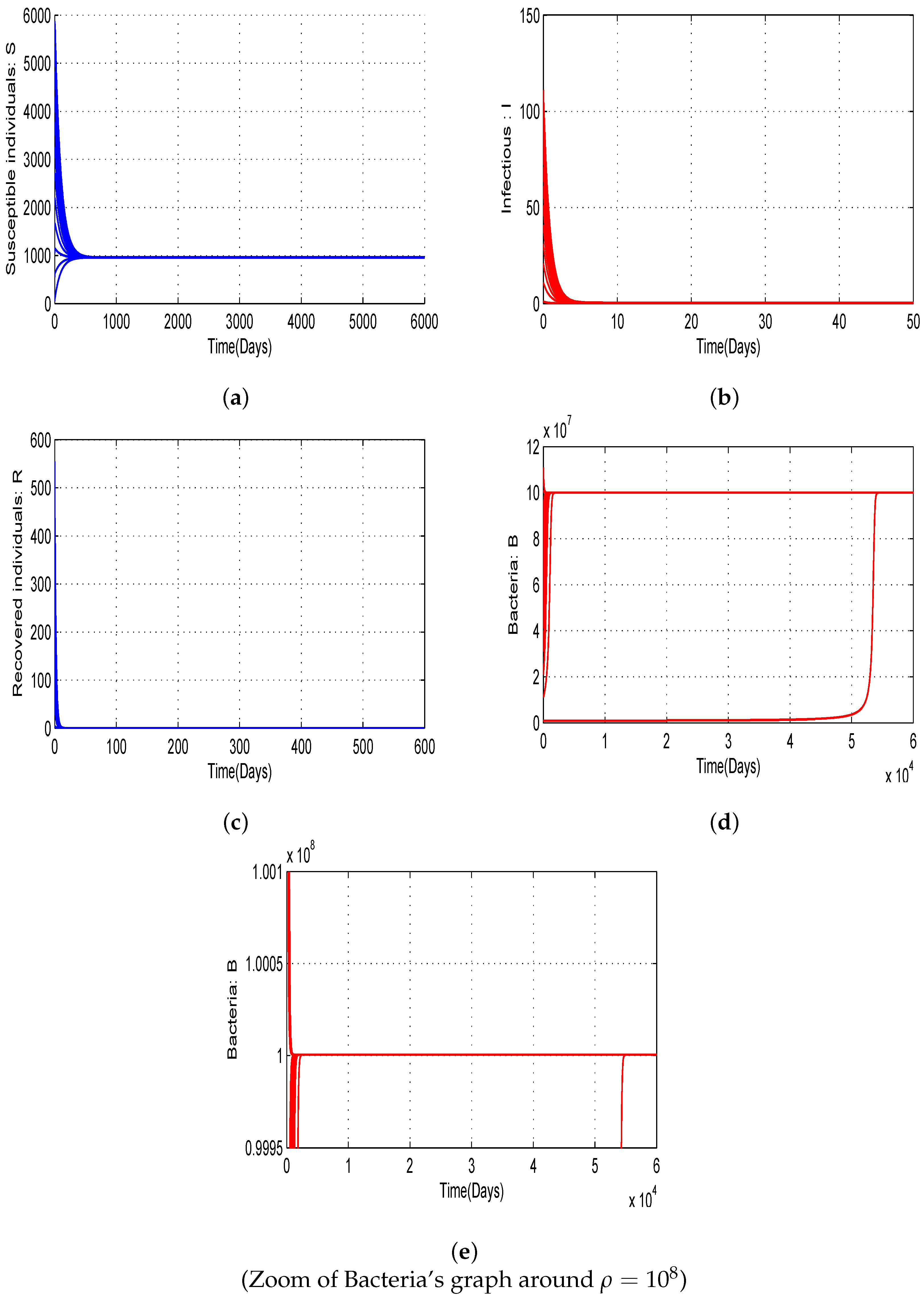
By Figure 4 global stability of Q ρ in Ω θ ϵ is also illustrated. Considering d = 0.7 , γ = 0.5 , α = 0.45 , and the remaining parameters are consistent with those listed in Table 1, we obtain R 0 0 = 0.0058 , ξ = 0.0505 , and R 0 ( Q ρ ) = 0.0033 . Choosing various initial conditions in D 3 = ] 0 ; 50 , 000 ] × ] 0 ; 10 ] × ] 0 ; 50 ] × 0.9 × 10 6 , 1.2 × 10 8 . It is seen in Figure 4 that solutions of model (2) converge to Q ρ .

3.3.3. Endemic Equilibrium

Let Q * = ( S * , I * , R * , B * ) be a homogeneous endemic equilibrium of model (2) with S * , I * , R * , and B * satisfying the following equations:
Λ ( λ * + μ ) S * + γ R * = 0 , λ * S * ω I * = 0 , α I * ( μ + γ ) R * = 0 , r B * ( B * θ ) ( ρ B * ) + δ I * = 0 ,
where λ * = β B * K + B * . Expressing endemic states S * and R * as a function of I * and λ * gives:
S * = ω λ * I * and R * = α μ + γ I * .
Using Equation (24) and the first equation of model (2), one has
I * = λ * S * ω = λ * ω Λ μ ω μ I * + γ α μ ( μ + γ ) I * .
Using Equation (25), one can deduce that
I * = Λ ( μ + γ ) λ * μ ω + γ ( μ + d ) λ * + ω μ ( μ + γ ) .
Using expression λ * = β B * K + B * in Equation (26) we obtain:
I * = Λ ( μ + γ ) β B * μ ω + γ ( μ + d ) β + ω μ ( μ + γ ) B * + ω μ ( μ + γ ) K .
Using Equation (27) in the last equation of (23) we obtain the following equation in B * :
a 3 B * 3 + a 2 B * 2 + a 1 B * + a 0 = 0 ,
where
a 3 = r β μ ( μ + d + α ) + β γ ( μ + d ) + ( μ + d + α ) μ ( μ + γ ) , a 2 = r ( θ + ρ ) β μ ( μ + d + α ) + β γ ( μ + d ) + ( μ + d + α ) μ ( μ + γ ) r K ( μ + d + α ) μ ( μ + γ ) , a 1 = r θ ρ β μ ( μ + d + α ) + β γ ( μ + d ) + ( μ + d + α ) μ ( μ + γ ) + r K ( μ + d + α ) μ ( μ + γ ) ( θ + ρ ) , a 0 = r θ ρ ( μ + d + α ) K μ ( μ + γ ) ( R 0 0 1 ) .
Thus, positive endemic equilibria Q * are obtained by solving the cubic Equation (28) in B * and substituting the result (positive values of B * ) into the expression of λ * and deducing the values of other state variables using relation (24). It is worth noting that the coefficient a 3 is always negative. The coefficient a 0 is positive (negative) if R 0 0 is greater than (less than) unity, respectively. As is demonstrated in Appendix E, System (2) may have zero, one, two, or three interior equilibria, depending on parameter values. The various possibilities for the roots of Equation (28) are summarized in the following Lemma.
Lemma 4. 
Model (2) could have:
  • either one or three interior equilibria if R 0 0 > 1 ,
  • either zero or two endemic equilibria if R 0 0 < 1 .
Lemma 5. 
For every positive solution B 0 * of polynomial Equation (28), we have B 0 * ] 0 ; θ [ ] ρ ; B m [ .
Proof. 
The proof of Lemma 5 is straightforward and evident. Let B 0 * be a solution of polynomial Equation (28). Suppose that B 0 * ] θ ; ρ [ . Consider Q 0 * = ( S 0 * , I 0 * , R 0 * , B 0 * ) , the endemic equilibrium state deduced from Equations (26) and (24). Using the last equation of (23) we have:
I 0 * = r δ B 0 * ( B 0 * θ ) ( ρ B 0 * ) < 0 which   is   impossible .
Now, using the center manifold theory, we are going to show that if ξ < R 0 0 < 1 and for a certain set of model parameters, model (2) has exactly two endemic equilibria, with one stable and another one unstable. To achieve this, we applied the Theorem of Castillo-Chavez and Song [22]. We have the following result.
Theorem 4. 
Model (2) undergoes a backward bifurcation at R 0 0 = 1 if the coefficient a defined as in Equation (A6) is positive, otherwise a < 0 there exists an endemic equilibrium Q * which is locally asymptotically stable for R 0 0 > 1 but close to 1.
The proof of Theorem 4 is given in Appendix C.
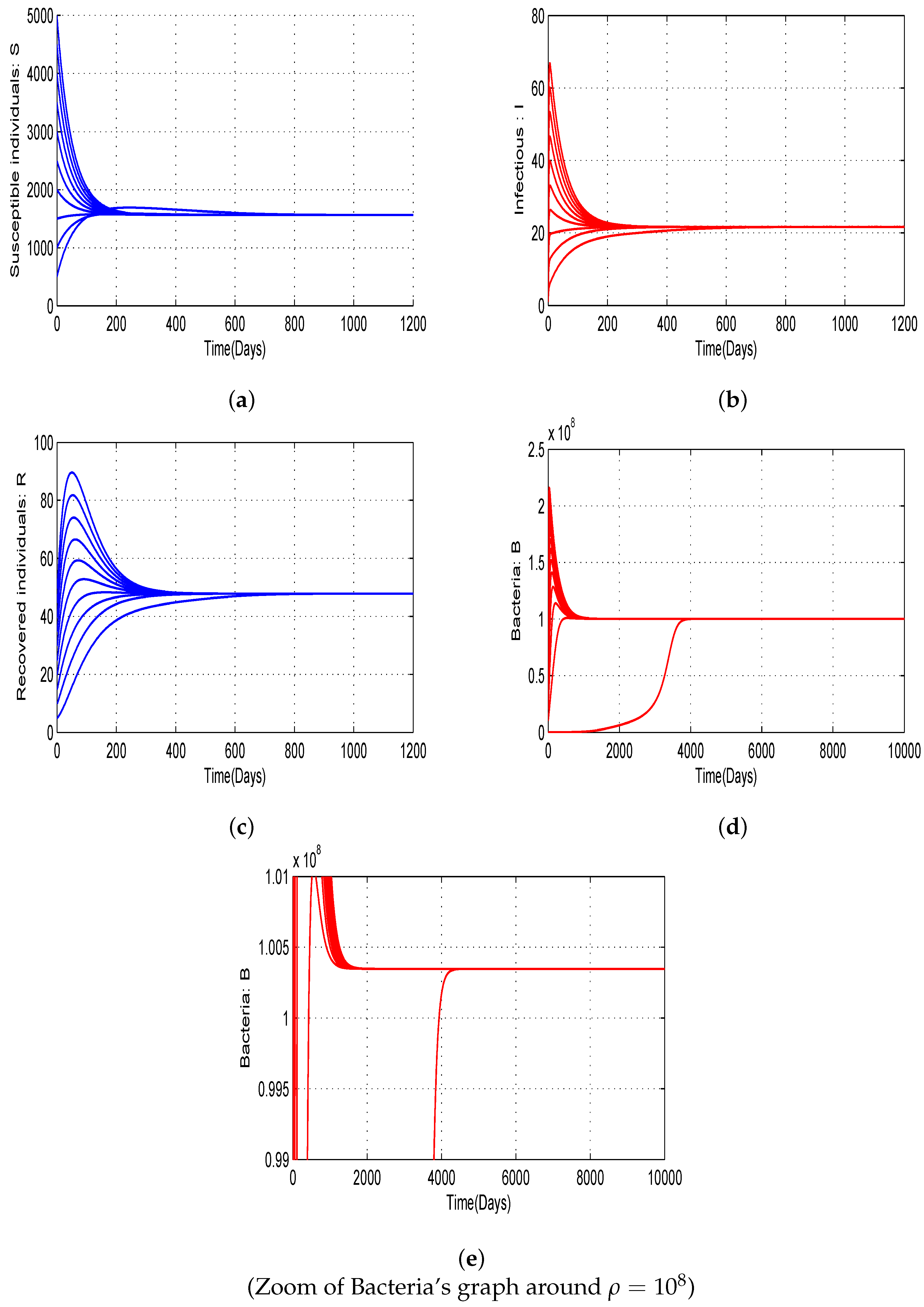
Figure 5 shows time series of model (2) when Λ = 30 , β = 0.01 (so that R 0 0 = 3.0809 > 1 ) and the remaining parameters are consistent with those listed in Table 1. Various initial condition have been taken in D 3 = ] 0 ; 7.5 × 10 6 ] × ] 0 ; 1.5 × 10 3 ] × ] 0 ; 7.5 × 10 3 ] × 10 5 , 1.5 × 10 8 . It clearly appears that the trajectories of model converge to an unique endemic equilibrium belonging to Ω ρ . This means that cholera persists within the community and the disease is uncontrollable.
To derive the stability region of any endemic equilibrium when R 0 0 1 , we applied the methods in van den Driessche and Watmough [21] once again. We found the basic reproduction number of infectious in a population where endemic equilibrium Q * = ( S * , I * , R * , B * ) is fixed (see Appendix D for details):
R 0 ( Q * ) = β K δ S * ( K + B * ) 2 ω ( r θ ρ 2 r ( θ + ρ ) B * + 3 r ( B * ) 2 ) .
According to the van den Driessche and Watmough [21] methods, this endemic equilibrium is locally asymptotically stable when R 0 ( Q * ) < 1 .
Now,
R 0 ( Q * ) < 1 R 0 0 S * S 0 K K + B * 2 r θ ρ < r θ ρ 2 r ( θ + ρ ) B * + 3 r ( B * ) 2 .
Thus,
R 0 ( Q * ) < 1 R 0 0 r θ ρ < r θ ρ 2 r ( θ + ρ ) B * + 3 r ( B * ) 2 0 < 3 r ( B * ) 2 2 r ( θ + ρ ) B * r θ ρ ( R 0 0 1 ) B * ] 0 ; B 1 * [ ] B 2 * ; B m [ ,
where
B 1 * = 1 3 θ + ρ ( ρ θ ) 2 + θ ρ + 3 θ ρ R 0 0 and B 2 * = 1 3 θ + ρ + ( ρ θ ) 2 + θ ρ + 3 θ ρ R 0 0
Considering B 1 * > 0 , we get R 0 0 < 1 . Since we have assumed that R 0 0 1 this imply that B 1 * 0 and consequently B * ] B 2 * ; B m [ .
One has
B 2 * = 1 3 θ + ρ + ( ρ θ ) 2 + θ ρ + 3 θ ρ R 0 0 > 1 3 2 θ + θ 2 + ρ ( ρ θ ) + 3 θ ρ R 0 0 > θ .
Considering Lemma 5, we get B * ] ρ ; B m [ . We have the following result:
Proposition 4. 
If R 0 0 1 , then any stable endemic equilibrium Q * = ( S * , I * , R * , B * ) of model (2) verifies B * ρ ; B m .
Now, what would happen if R 0 ( Q ρ ) 1 ? The contrapositive of Proposition 3 gives:
If R 0 ( Q ρ ) 1 , then ϵ 0 ; θ , R 0 0 ξ .
This implies the existence of one stable endemic equilibrium for model (2) in Ω .
Theorem 5. 
There exists an endemic equilibrium Q * which is locally asymptotically stable when R 0 ( Q ρ ) > 1 but close to 1.
The proof of Theorem 5 is given in Appendix C.

4. Discussion

This section presents two main simulations: numerical simulations of the model, and numerical simulations of the threshold quantities.

4.1. Numerical Simulations of the Proposed Model with Variation of Threshold Quantities

It is important to have a global view of dynamic on model (2) when various initial conditions are taken in R + 4 and when threshold quantity R 0 0 and R 0 ( Q ρ ) are varying around critical values (unity and value of ξ ). Therefore, four cases will be examined through graphs of bacteria and infected population.
Case 1:  R 0 ( Q ρ ) < 1 < R 0 0
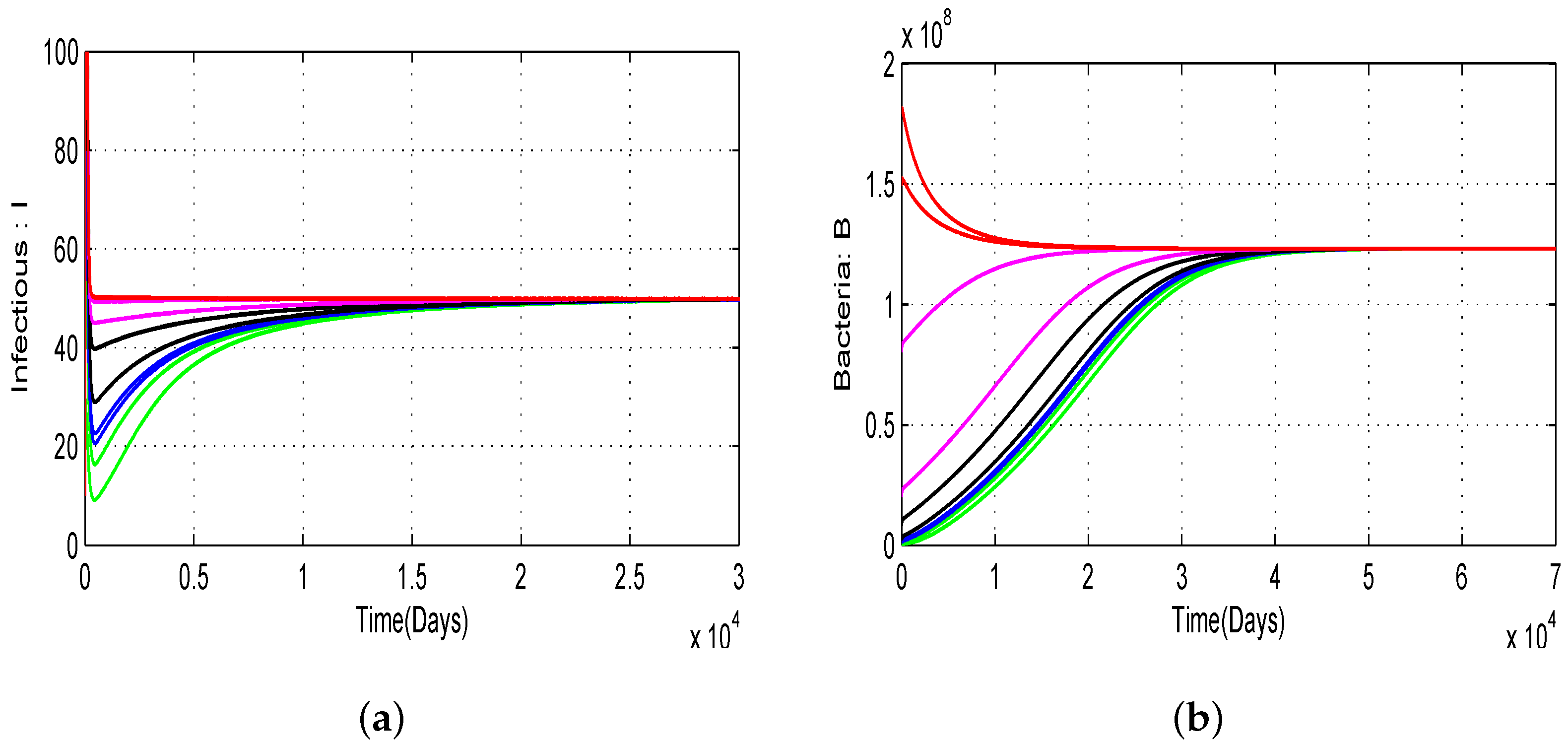
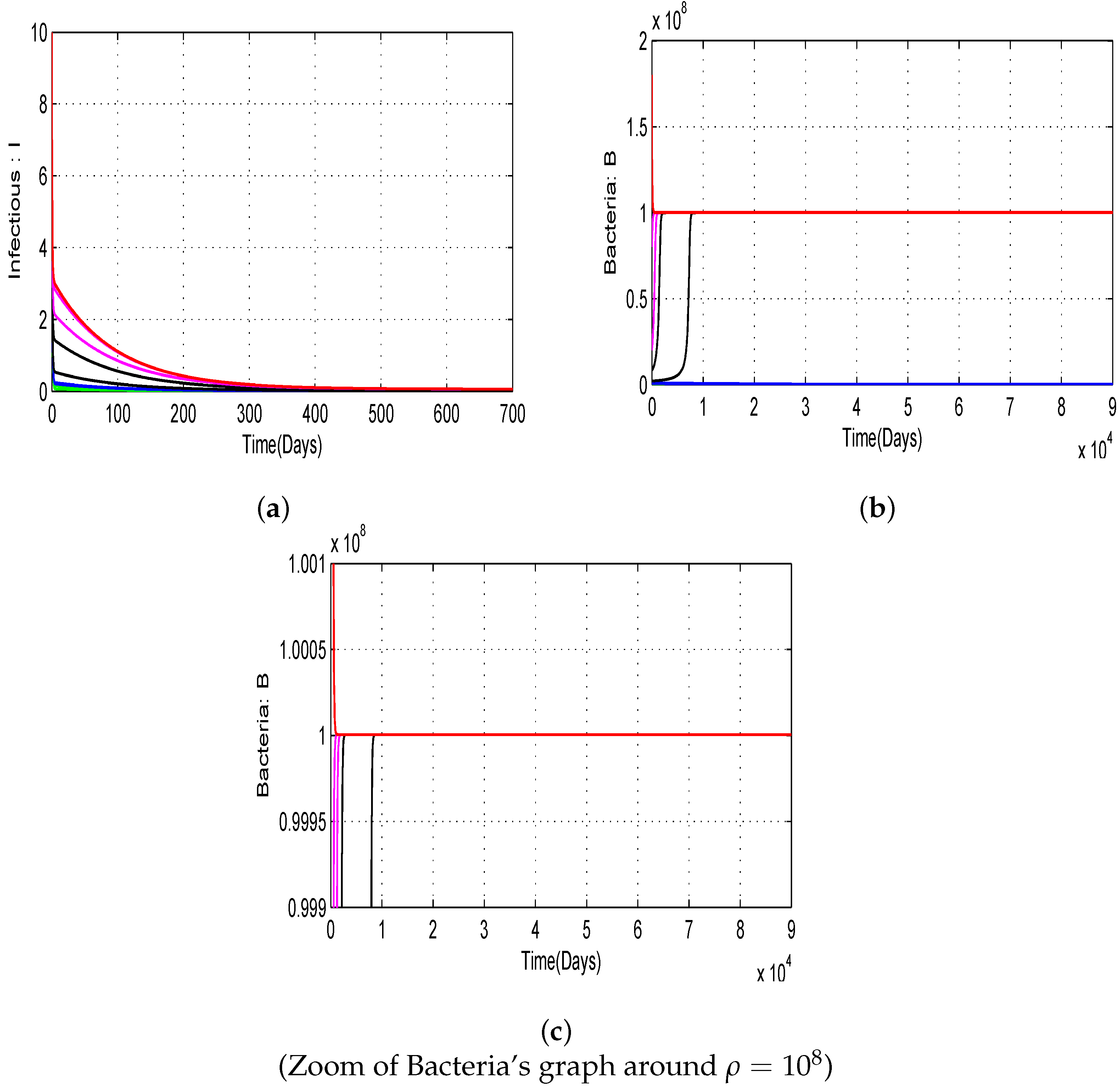
To get R 0 ( Q ρ ) < 1 < R 0 0 we can fix Λ = 50 , β = 0.02 and r = 10 20 (so that R 0 ( Q ρ ) = 0.0526 and R 0 0 = 1.7594 × 10 3 ) and the remaining parameters are consistent with those listed in Table 1. The numerical simulations obtained in Figure 6 show that all the solutions of model (2) converge to an endemic equilibrium. It is therefore numerically observed that the instability of Q 0 also implies instability of Q ρ .
Case 2:  R 0 ( Q ρ ) < R 0 0 < ξ < 1
According to Theorems 2 and 3, case 2 should illustrate the convergence to Q 0 or Q ρ of every solution of model (2) when initial conditions are taken in their attraction domain respectively. Figure 7 is obtained by considering parameter values in Table 1 with ϵ = 50 , 000 .
For these values we have R 0 ( Q ρ ) = 0.0023 , R 0 0 = 0.0045 and ξ = 0.0495 . Extinction of the infectious agent does not depend on the initial conditions. Extinction of population of bacteria is obtained when initial values are chosen in D 3 = ] 0 ; 50 , 000 ] × ] 0 ; 10 ] × ] 0 ; 50 ] × [ 10 5 , 9.9 × 10 5 ] . Saturation of the bacterial population is obtained for initial conditions chosen in D 4 = ] 0 ; 50 , 000 ] × ] 0 ; 10 ] × ] 0 ; 50 ] × 10 6 , 2 × 10 8 .
Case 3:  ξ < R 0 ( Q ρ ) < R 0 0 < 1
The phenomenon of backward bifurcation occurs. But the fact that an stable equilibrium endemic exists in Ω ρ implies consequent instability of Q ρ even if R 0 ( Q ρ ) < 1 . The simulations of Figure 8 are obtained when Λ = 30 , β = 0.001 and ϵ = 1000 (so that ξ = 0.0010 , R 0 ( Q ρ ) = 0.027 , and R 0 0 = 0.308 ).
Extinction of epidemic and population of bacteria are obtained for initial values chosen in D 5 = ] 0 ; 50 , 000 ] × ] 0 ; 10 ] × ] 0 ; 50 ] × 0 , 5 × 10 5 . The endemicity situation is observed for initial values chosen in D 6 = ] 0 ; 50 , 000 ] × ] 0 ; 10 ] × ] 0 ; 50 ] × 7 × 10 5 , 2 × 10 8 .
Case 4:  ξ < R 0 0 < 1 < R 0 ( Q ρ )
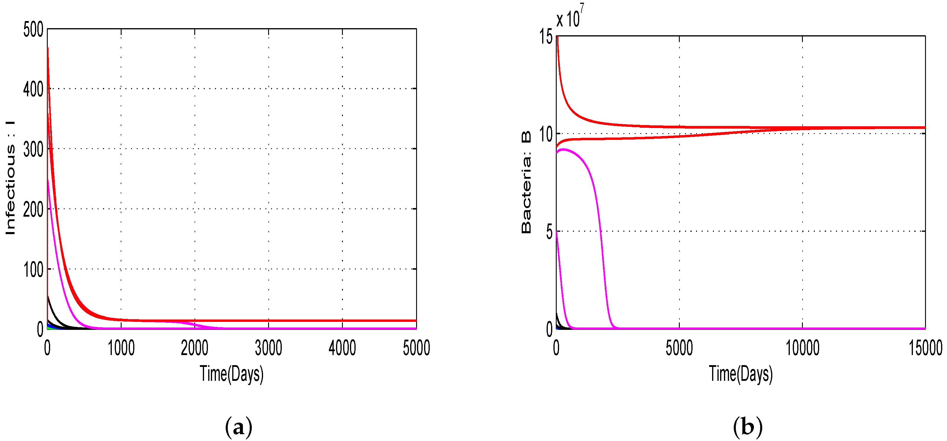
The following parameters are modified β = 0.1 , μ = 1.04 × 10 3 , θ = 0.999 × 10 8 and ϵ = 50 , 000 (so that ξ = 5.005 × 10 8 , R 0 0 = 0.0104 and R 0 ( Q ρ ) = 4.5370 ). This is illustrated in Figure 9 where we can see the previous situation.
From these different cases, it is easy to project the dynamics of model (2) in other situations.

4.2. Numerical Simulations of Threshold Quantities with Variation of Allee Parameters θ and ρ and Bifurcation

The theoretical findings presented in Section 3.3 corroborate the biological and epidemiological evidence that bacterial growth plays a critical role in cholera emergence [23]. Our model (2) captures this growth mathematically through a dynamic that incorporates the Allee effect, allowing us to represent the distinct phases of bacterial growth fluctuations resulting from environmental variations. These phases are characterized by the parameters θ and ρ , which correspond to the Allee threshold and carrying capacity of bacteria, respectively.
The significance of these parameters in determining bacterial growth in the environment highlights the need for a comprehensive analysis of their impact on cholera persistence and extinction through rigorous simulations.
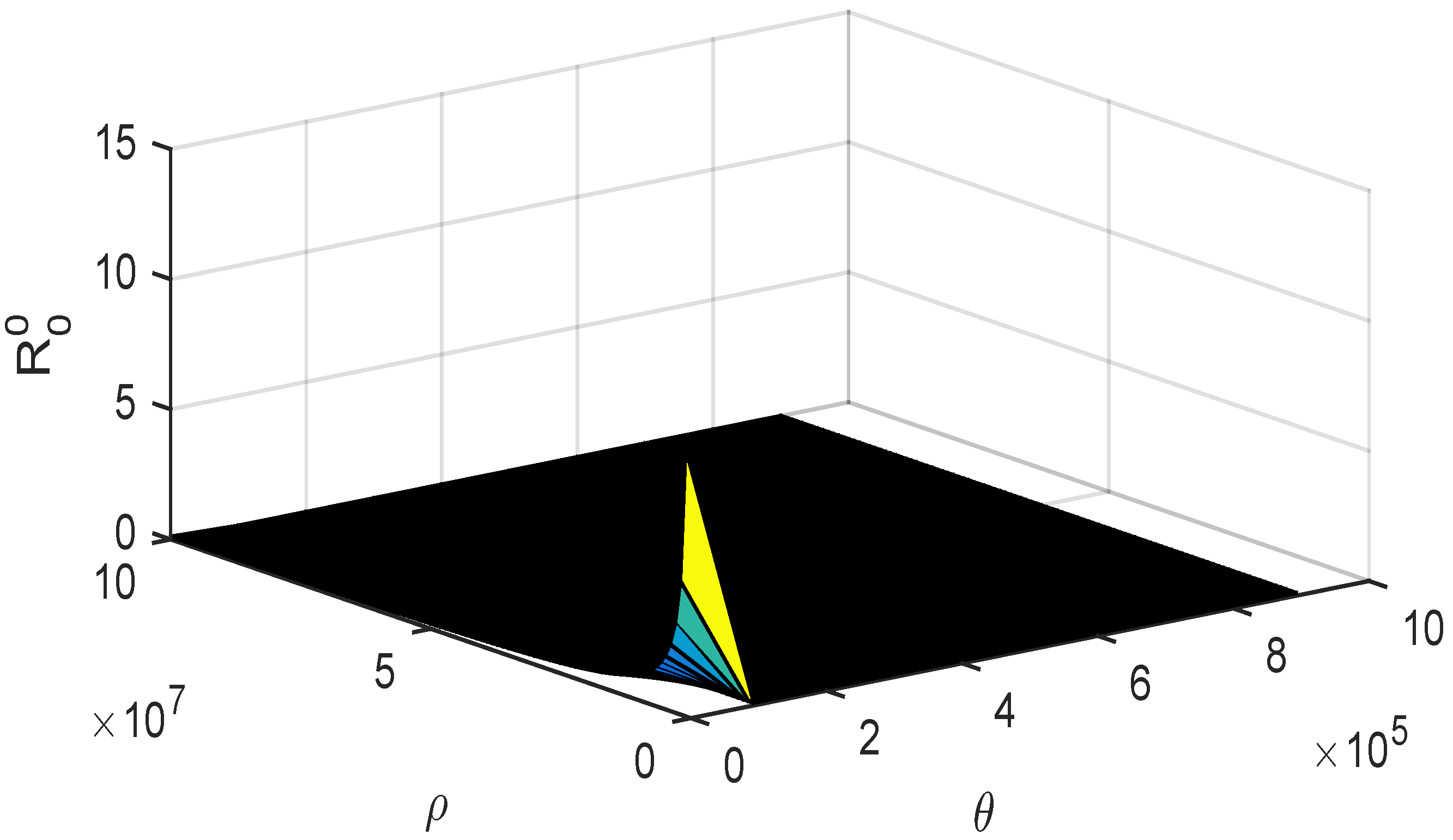
A three-dimensional simulation depicting the relationship between the basic reproduction number R 0 0 , and the Allee effect parameters ( θ and ρ ) is presented in Figure 10.
It is evident that the basic reproductive number R 0 0 approaches zero as θ exceeds 10 5 . This indicates that the likelihood of disease outbreaks is significantly reduced when the Allee effect threshold is above 10 5 in this scenario.
In Figure 11, we present variations of R 0 ( Q ρ ) for some values of θ and ρ :
  • The curves obtained highlight the importance of emphasizing that the risk of disease outbreaks cannot be neglected for any value of θ .
  • Additionally, as θ approaches ρ , the probability of epidemic outbreaks significantly increases.
Figure 11. Simulation of R 0 ( Q ρ ) for various values of θ [ 0 ; 10 6 ] and ρ [ 10 6 ; 10 7 ] when Λ = 70 , β = 0.001 and the remaining parameters are consistent with those listed in Table 1.
Sustainability 15 10384 g011
Figure 12 displays the range of values for θ and ρ in which the conditions R 0 0 = ξ (with a fixed ϵ ) and R 0 ( Q ρ ) = 1 are simultaneously satisfied: Figure 12a,b are obtained for ϵ = 1 and ϵ = 50 , 000 , respectively. By considering various values of ϵ within the interval ( 0 , θ ) , it is evident that the conditions R 0 0 < ξ and R 0 ( Q ρ ) < 1 are almost indistinguishable when ϵ exceeds 50.
The numerical results presented in Figure 12 support the theoretical Proposition outlined in Proposition 3, which asserts that the stability condition of Q 0 also implies that of Q ρ .
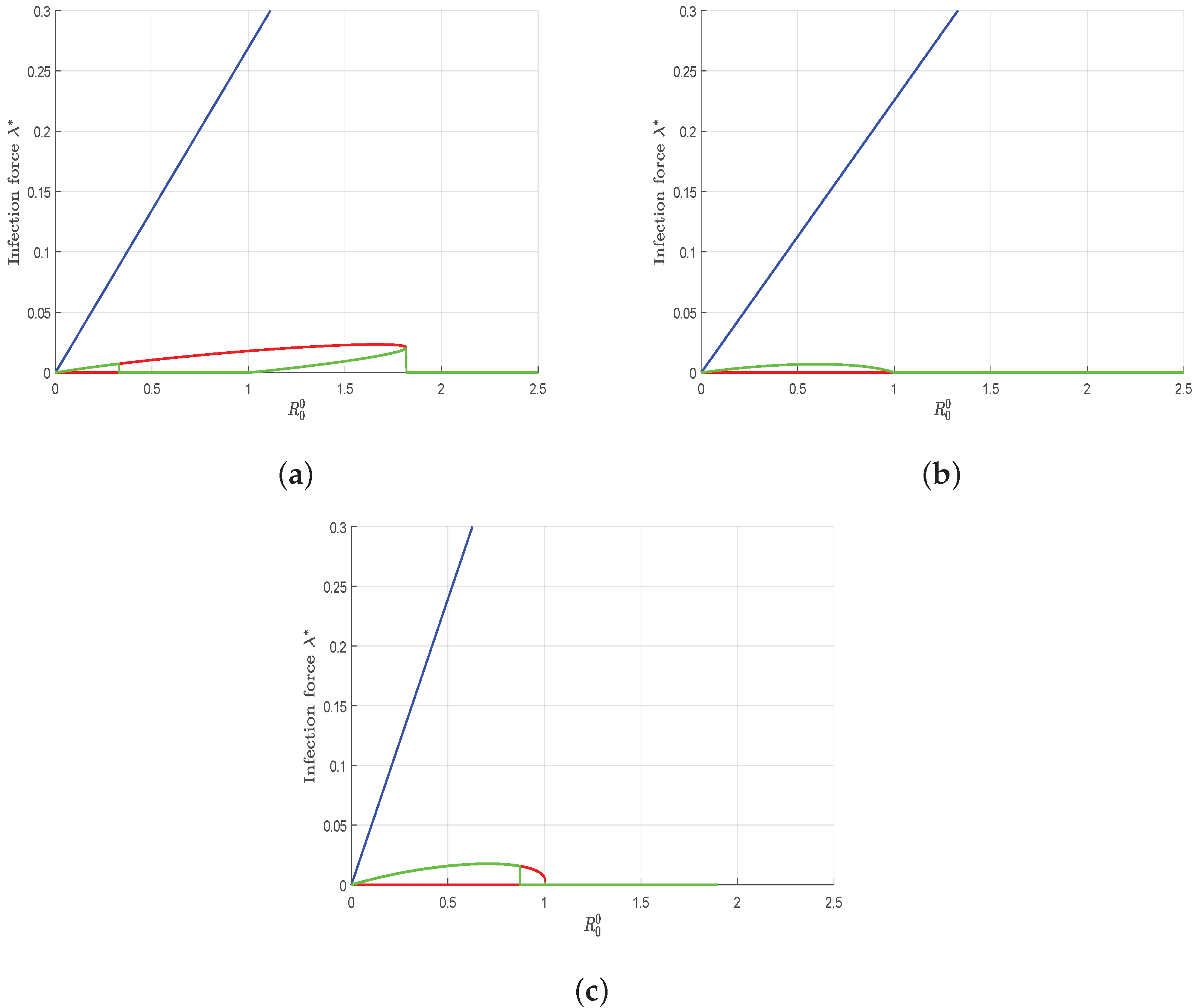
It was stated in Theorem 4 that the model undergoes a bifurcation at R 0 0 = 1 . When we vary parameter value R 0 0 around unity through parameter β (the remaining parameters are fixed) of model (2), we obtain for each value of β different solutions of polynomial Equation (28) which permit us to deduce different persistent infection forces.
Figure 13 provides visual confirmation of the findings presented in Lemma 4 which highlights how the number of equilibrium points of model (2) varies with changing parameters. The illustration serves as a visual aid for the discussion and provides empirical evidence that supports the theoretical underpinnings of the Lemma.

5. Conclusions

The principal aim of this study was to comprehensively analyze the impact of environmental factors on the dynamics of bacterial populations via the Allee effect. Existing models in the literature often suffer from unrealistic assumptions, such as linear or logistic growth of bacteria, which fail to consider the complex dynamics of bacterial populations. In this work, we proposed a novel S-I-R-S epidemic model for cholera transmission that takes into account multiple crucial factors, including the Allee effect in bacterial reproduction, loss of immunity in recovered individuals, and logistic dose-response of bacteria on infection force to cholera. The model exhibits three DFEs, each corresponding to a distinct epidemiological scenario. The Q 0 equilibrium represents the ideal situation where there are no infected individuals, and the bacterial concentration is extremely low. The Q θ equilibrium represents the critical scenario under which the disease and bacteria may disappear if the basic reproduction number is below a certain threshold and the initial conditions are within the attraction domain of Q 0 . However, when the bacterial concentration exceeds the value of θ , the solutions of the model converge to Q ρ or an endemic equilibrium, depending on the value of the basic reproduction number. The Q ρ equilibrium corresponds to a situation where bacteria are present in the environment without any infected individuals, which is a common occurrence in endemic regions in Africa, such as Cameroon. Our findings can be summarized as follows:
  • The model exhibits three disease-free equilibria related to three different real situations.
  • The dynamics of the proposed model are determined by the threshold quantity R 0 0 .
  • The phenomenon of bi-stability is observed, with backward and forward bifurcation.
  • This research demonstrates that the Allee effect provides a robust framework for characterizing fluctuations in bacterial populations and the onset of cholera outbreaks
Sensitivity analysis of the model revealed that parameters related to human–bacteria contact and bacterial dynamics significantly affect the global dynamics of the model. Hence, during an epidemic situation, it is imperative to conduct awareness campaigns on hygiene practices and initiate sanitation campaigns in high-risk areas. Finally, the numerical simulations presented in this study support the theoretical findings and demonstrate the stability of the DFEs and the existence and stability of the endemic equilibrium. Future improvements and extensions of the model include expanding it to multiple patches and integrating time-dependent parameters to account for periodic variations in environmental factors.

Author Contributions

Conceptualization, G.K.G. and S.B.; formal analysis, G.K.G. and R.H.N.; investigation, M.-A.A.-A., S.B. and R.H.N.; methodology, G.K.G., S.B. and M.-A.A.-A.; project administration, R.H.N. and S.B.; software, G.K.G. and B.A.; supervision, M.-A.A.-A.; validation, R.H.N. and M.-A.A.-A.; writing—original draft preparation, G.K.G.; visualization: R.H.N.; writing—review and editing, B.A., R.H.N. and M.-A.A.-A. All authors have read and agreed to the published version of the manuscript.

Funding

The authors would like to express their gratitude for the financial support provided by IMU-SIMONS African towards this research.

Institutional Review Board Statement

Not applicable.

Informed Consent Statement

Not applicable.

Data Availability Statement

Data used in this article were simulated and can be made available on demand.

Conflicts of Interest

The authors declare no financial or non-financial competing interest.

Abbreviations

The following abbreviations are used in this manuscript:
DFEDisease-Free Equilibrium
GASGlobal Asymptotic Stability
LHSLatin Hypercube Sampling
PRCCPartial Rank Correlation Coefficients
SIRSusceptible Infected Recovered
VNCViable but Non-Culturable

Appendix A. Calculation of Persistence Threshold for Disease-Free Equilibrium

Considering the disease-free equilibrium Q ρ = ( S ρ , 0 , 0 , ρ ) and using the notations in van den Driessche and Watmough [21] for model (2) the matrices F and V for the new infection terms and the remaining transfer terms are, respectively, given by:
F = 0 β K Λ ( k + ρ ) [ β ρ + μ ( ρ + K ) ] 0 0 and V = ω 0 δ r ρ ( ρ θ ) .
Following van den Driessche and Watmough [21], the basic reproduction number of infections in population where Q ρ is fixed is then the spectral radius of the next generation matrix F V 1 ,
R 0 ( Q ρ ) = β K δ Λ [ β ρ + μ ( ρ + K ) ] ( K + ρ ) ω r ρ ( ρ θ )

Appendix B. Proof of Lemma 4

The number of positive roots of (28) determines the number of endemic equilibria of model (2). In order to identify the number of endemic equilibria, we require the partial derivative of function P : B * a 3 B * 3 + a 2 B * 2 + a 1 B * + a 0 with respect to B * which is given by:
d P ( B * ) d B * = 3 a 3 ( B * ) 3 + 2 a 2 ( B * ) 2 + a 1 .
Thus, when Δ = 4 a 2 2 12 a 1 a 3 > 0 , equation d P ( B * ) d B * = 0 has two real roots v i , i = 1 , 2 given by:
v 1 = 2 a 2 4 a 2 2 12 a 1 a 3 6 a 3 and v 2 = 2 a 2 + 4 a 2 2 12 a 1 a 3 6 a 3 .
Therefore, we conclude that:
  • if R 0 0 > 1 model (2) has:
    • one endemic equilibrium if ( v 1 < v 2 < 0 , P ( v 2 ) > 0 ) or if ( v 1 < 0 < v 2 , P ( v 2 ) > 0 ) or if ( v 2 > v 1 > 0 , P ( v 1 ) < 0 , P ( v 2 ) < 0 ) or if ( v 2 > v 1 > 0 , P ( v 1 ) > 0 , P ( v 2 ) > 0 ),
    • three endemic equilibria if ( v 2 > v 1 > 0 , P ( v 1 ) < 0 , P ( v 2 ) > 0 ).
  • if R 0 0 < 1 model (2) has:
    • no endemic equilibrium if ( 0 < v 1 < v 2 , P ( v 1 ) < 0 , P ( v 2 ) < 0 ) or if ( v 1 < v 2 < 0 , P ( v 1 ) < 0 ) or if ( v 1 < v 2 < 0 , P ( v 1 ) > 0 , P ( v 2 ) > 0 ) or if ( v 1 < 0 < v 2 , P ( v 1 ) < 0 , P ( v 2 ) < 0 ),
    • two endemic equilibria if ( v 1 < 0 < v 2 , P ( v 1 ) < 0 , P ( v 2 ) > 0 ) or if ( 0 < v 1 < v 2 , P ( v 1 ) < 0 , P ( v 2 ) > 0 ).

Appendix C. Proof of Theorem 4

We present the proof of Theorem 4 on the local stability of the endemic equilibrium point of model (2) when R 0 0 > 1 . To do so, the following simplification and change of variables are made first of all. Let x 1 = S , x 2 = I , x 3 = R , x 4 = B .
Further, by using the vector notation x = ( x 1 , x 2 , x 3 , x 4 ) , model (2) can be written in the form x ˙ = f ( x ) with f = ( f 1 , f 2 , f 3 , f 4 ) as follows:
x 1 ˙ = Λ λ + μ x 1 + γ x 3 , x 2 ˙ = λ x 1 ω x 2 , x 3 ˙ = α x 2 ( γ + μ ) x 3 , x 4 ˙ = r x 4 ( x 4 θ ) ( ρ x 4 ) + δ x 2 ,
where λ = β x 4 x 4 + K .
Model (A2) has a DFE given by Q 0 = S 0 , 0 , 0 , 0 where S 0 = Λ μ . The Jacobian of model (2) at the DFE Q 0 is
J ( Q 0 ) = μ 0 γ β * S 0 K 0 ω 0 β * S 0 K 0 α ( μ + γ ) 0 0 δ 0 r ρ θ .
The basic reproduction number of the transformed (linearized) model (A2) is the same as that of the original model given by Equation (2). Therefore, choosing β as a bifurcation parameter, solving for β from R 0 0 = 1 , we obtain:
β * = K r ρ θ μ ω Λ δ .
It follows that the Jacobian J ( Q 0 ) of model (A2) at the DFE Q 0 , with β = β * , denoted by J β * has a simple zero eigenvalue (with all other eigenvalues having negative real parts). Hence, the Centre Manifold theory [24] can be used to analyze the dynamics of model (A2). In particular, the Theorem of Castillo-Chavez and Song [22], reproduced below for convenience, will be used to show that when R 0 0 > 1 there exists an endemic equilibrium of model (A2) which is locally asymptotically stable for R 0 0 near 1 under certain conditions.
Theorem A1. 
(Castillo-Chavez and Song [22]). Consider the following general system of ordinary differential equations with a parameter Φ:
d z d t = f ( x , Φ ) , f : R n × R R and f C 2 ( R n × R ) ,
where 0 is an equilibrium point of the system (that is, f ( 0 , Φ ) 0 for all Φ) and assume
1. 
A = D z f ( 0 , 0 ) = f i z j ( 0 , 0 ) is the linearization matrix of model (A4) around the equilibrium 0 with Φ evaluated at 0. Zero is a simple eigenvalue of A and other eigenvalues of A have negative real parts;
2. 
Matrix A has a right eigenvector u and a center eigenvector v (each corresponding to the zero eigenvalue). Let f k be the k t h component of f and
a = k , i , j = 1 n v k u i u j 2 f k x i x j ( 0 , 0 ) and b = k , i = 1 n v k u i 2 f k x i Φ ( 0 , 0 ) ,
then, the local dynamics of the system around the equilibrium point 0 is totally determined by the signs of a and b.
1. 
a > 0 , b > 0 . When Φ < 0 with | Φ | 1 , 0 is locally asymptotically stable and there exists a positive unstable equilibrium; when 0 < Φ 1 , 0 is unstable and there exists a negative, locally asymptotically stable equilibrium;
2. 
a < 0 , b < 0 . When Φ < 0 with | Φ | 1 , 0 is unstable; when 0 < Φ 1 , 0, is locally asymptotically stable equilibrium, and there exists a positive unstable equilibrium;
3. 
a > 0 , b < 0 . When Φ < 0 with | Φ | 1 , 0 is unstable and there exists a locally asymptotically stable negative equilibrium; when 0 < Φ 1 , 0 is stable, and a positive unstable equilibrium appears;
4. 
a < 0 , b > 0 . When Φ changes from negative to positive, 0 changes its stability from stable to unstable. Correspondingly a negative unstable equilibrium becomes positive and locally asymptotically stable.
In order to apply the above Theorem, the following computations are necessary (it should be noted that we are using β * as the bifurcation parameter, in place of Φ in Theorem A1).
Eigenvectors of  J β *
For the case when R 0 0 = 1 , it can be shown that the Jacobian of model (A2) has a right eigenvector (corresponding to the zero eigenvalue), given by U = ( u 1 , u 2 , u 3 , u 4 ) T , where
u 1 = γ α μ ( μ + γ ) ω μ u 2 , u 2 = u 2 > 0 , u 3 = α μ + γ u 2 , and u 4 = δ r ρ θ u 2 .
Similarly, the components of the center eigenvectors of J β * (corresponding to the zero eigenvalue), denoted by V = ( v 1 , v 2 , v 3 , v 4 ) T , are given by:
v 1 = 0 , v 2 = v 2 > 0 , v 3 = 0 , and v 4 = β S 0 K r ρ θ v 2 .
Computation of b 
For the sign of b, it can be shown that the associated non-vanishing partial derivatives of f are:
2 f 1 x 4 β * ( 0 , 0 ) = S 0 K and 2 f 2 x 4 β * ( 0 , 0 ) = S 0 K .
It follows that:
b = ω β * v 2 u 2 > 0 .
Computation of a 
For system (A2), the associated non-zero partial derivatives of f (at the DFE Q 0 ) are given by:
2 f 1 x 1 x 4 ( 0 , 0 ) = β * K , 2 f 1 x 4 2 ( 0 , 0 ) = 2 β * S 0 K , 2 f 2 x 1 x 4 ( 0 , 0 ) = β * K , 2 f 2 x 4 2 ( 0 , 0 ) = 2 β * S 0 K
and 2 f 4 x 4 2 ( 0 , 0 ) = 2 r ( ρ + θ ) .
Then, it follows that:
a = v 2 i , j = 1 4 u i u j 2 f 2 x i x j ( 0 , 0 ) + v 4 i , j = 1 4 u i u j 2 f 4 x i x j ( 0 , 0 ) , = v 2 u 2 2 α γ ω ( μ + γ ) S 0 + 2 ω K β * S 0 2 ω δ r ( ρ + θ ) ω S 0 1 μ + 2 K β * .
Thus, depending on the values of the parameters of model (2), the value of a can be positive or negative. So, if b > 0 , if a > 0 , model (2) undergoes the phenomenon of backward bifurcation (see Theorem A1, item (1)). Also, if a < 0 (by Theorem A1, item (4)), we have established the result about the local stability of the endemic equilibrium Q * of model (2) for R 0 0 > 1 but close to 1.
This concludes the proof of Theorem 4.

Appendix D. Calculation of Persistence Threshold for Endemicity

Consider any endemic equilibrium Q * = ( S * , I * , R * , B * ) .
Suppose cholera is transmissible in the population at point Q * . Using the notations in van den Driessche and Watmough [21] for model (2), the matrices F and V for the new infection terms and the remaining transfer terms are, respectively, given by:
F = 0 β K S * ( k + B * ) 2 0 0 and V = ω 0 δ r θ ρ 2 r ( θ + ρ ) B * + 3 r ( B * ) 2 .
Following van den Driessche and Watmough [21], the basic reproduction number of infections in population where Q * is fixed is then the spectral radius of the next generation matrix F V 1 ,
R 0 ( Q * ) = β K δ S * ( K + B * ) 2 ω ( r θ ρ 2 r ( θ + ρ ) B * + 3 r ( B * ) 2 ) .

Appendix E. Proof of Theorem 5

The proof will be the same as in Appendix C. Let us make the following simplification and change of variables: Let y 1 = S , y 2 = I , y 3 = R , y 4 = B . Further, by using the vector notation y = ( y 1 , y 2 , y 3 , y 4 ) , model (2) can be written in the form y ˙ = g ( y ) with g = ( g 1 , g 2 , g 3 , g 4 ) as follows:
y 1 ˙ = Λ λ + μ y 1 + γ y 3 , y 2 ˙ = λ y 1 ω y 2 , y 3 ˙ = α y 2 ( γ + μ ) y 3 , y 4 ˙ = r y 4 ( y 4 θ ) ( ρ y 4 ) + δ y 2 ,
where λ = β y 4 y 4 + K . System (A8) has a DFE given by Q ρ = S 0 , 0 , 0 , ρ where S ρ = Λ ( ρ + K ) β ρ + μ ( ρ + K ) . The Jacobian of model (2) at the DFE Q ρ is:
J ( Q ρ ) = μ β ρ ρ + K 0 γ β K Λ ( k + ρ ) [ β ρ + μ ( ρ + K ) ] β ρ ρ + K ω 0 β K Λ ( k + ρ ) [ β ρ + μ ( ρ + K ) ] 0 α ( μ + γ ) 0 0 δ 0 r ρ ( ρ θ ) .
Therefore, choosing β as a bifurcation parameter and solving for β from R 0 ( Q ρ ) = 1 , we obtain:
β = β * = ( K + ρ ) ω r ρ ( ρ θ ) [ β ρ + μ ( ρ + K ) ] Λ K δ .
It follows that the Jacobian J ( Q ρ ) of model (2) at the DFE Q ρ , denoted by simple J β * has a simple zero eigenvalue (with all other eigenvalues having negative real parts).
Eigenvectors of  J β *
For the case when R 0 ( Q ρ ) = 1 , it can be shown that the Jacobian of model (A8) has a right eigenvector (corresponding to the zero eigenvalue), given by U = ( u 1 , u 2 , u 3 , u 4 ) T , where
u 1 = 0 , u 2 = u 2 > 0 , u 3 = α μ + γ u 2 , and u 4 = δ r ρ ( ρ θ ) u 2 .
Similarly, the components of the center eigenvectors of J β * (corresponding to the zero eigenvalue), denoted by V = ( v 1 , v 2 , v 3 , v 4 ) T , are given by:
v 1 = v 1 > 0 ,
v 2 = [ β ρ + μ ( ρ + K ) ] β ρ v 1 ,
v 3 = γ γ + μ v 1 ,
v 4 = ω [ β ρ + μ ( ρ + K ) ] β ρ α γ γ + μ v 1 δ .
Computation of b: 
For the sign of b, it can be shown that the associated non-vanishing partial derivatives of f are:
2 g 1 y 1 β * ( 0 , 0 ) = ρ K + ρ ,
2 g 1 y 1 β * ( 0 , 0 ) = K Λ ( k + ρ ) [ β ρ + μ ( ρ + K ) ] ,
2 g 2 y 1 β * ( 0 , 0 ) = ρ K + ρ .
and 2 g 2 y 1 β * ( 0 , 0 ) = K Λ ( k + ρ ) [ β ρ + μ ( ρ + K ) ] .
It follows that:
b = μ ( K + ρ ) ω β * ρ u 2 > 0 .
Computation of a: 
For system (A8), the associated non-zero partial derivatives of g (at the DFE Q ρ ) are given by:
2 g 1 x 1 x 4 ( 0 , 0 ) = β * K ( K + ρ ) 2 ,
2 g 1 2 x 4 ( 0 , 0 ) = 2 β * K Λ ( K + ρ ) 2 [ β ρ + μ ( ρ + K ) ] ,
2 g 2 x 1 x 4 ( 0 , 0 ) = β * K ( K + ρ ) 2 g ,
and 2 g 1 2 x 4 ( 0 , 0 ) = 2 β * K Λ ( K + ρ ) 2 [ β ρ + μ ( ρ + K ) ] .
Then, it follows that:
a = δ r ρ ( ρ θ ) 2 2 β * K Λ μ ( K + ρ ) [ β ρ + μ ( ρ + K ) ] β * ρ + ω [ β ρ + μ ( ρ + K ) ] β ρ δ α γ ( γ + μ ) δ v 1 u 2 2 < 0 .
Thus, the a < 0 and b > 0 model (2) undergoes the phenomenon of forward bifurcation (see Theorem A1, item (4)).
So, we have established the result about the local stability of the endemic equilibrium of cholera disease model when Q ρ is suppose be a disease-free equilibrium (note that this result holds for R 0 ( Q ρ ) > 1 but close to 1).
This concludes the proof of Theorem 5.

References

  1. World Health Organization, Cholera. Available online: https://www.who.int/news-room/fact-sheets/detail/cholera. (accessed on 30 March 2023).
  2. Lipp, E.K.; Huq, A.; Colwell, R.R. Effects of global climate on infectious disease: The cholera model. Clin. Microbiol. Rev. 2002, 15, 757–770. [Google Scholar] [CrossRef] [PubMed] [Green Version]
  3. Islam, M.S.; Drasar, B.S.; Sack, R.B. The aquatic environment as a reservoir of Vibrio cholerae: A review. J. Diarrhoeal Dis. Res. 1993, 11, 197–206. [Google Scholar] [PubMed]
  4. Kolaye, G.; Bowong, S.; Houe, R.; Aziz-Alaoui, M.A.; Cadivel, M. Mathematical assessment of the role of environmental factors on the dynamical transmission of cholera. Commun. Nonlinear Sci. Numer. Simul. 2019, 67, 203–222. [Google Scholar] [CrossRef] [Green Version]
  5. Codeço, C.T. Endemic and epidemic dynamics of cholera: The role of the aquatic reservoir. BMC Infect. Dis. 2001, 1, 1. [Google Scholar] [CrossRef] [PubMed] [Green Version]
  6. Hartley, D.M.; Morris, J.G., Jr.; Smith, D.L. Hyperinfectivity: A critical element in the ability of V. cholerae to cause epidemics? PLoS Med. 2006, 3, e7. [Google Scholar] [CrossRef] [PubMed]
  7. Kolaye, G.; Damakoa, I.; Bowong, S.; Houe, R.; Békollè, D. Theoretical assessment of the impact of climatic factors in a Vibrio cholerae model. Acta Biotheor. 2018, 66, 279–291. [Google Scholar] [CrossRef] [PubMed] [Green Version]
  8. Kolaye, G.; Damakoa, I.; Bowong, S.; Houe, R.; Békollè, D. A mathematical model of cholera in a periodic environment with control actions. Int. J. Biomath. 2020, 13, 2050025. [Google Scholar] [CrossRef]
  9. Colwell, R.; Brayton, P.; Grimes, D.; Roszak, D.; Huq, S.; Palmer, L. Viable but non-culturable Vibrio cholerae and related pathogens in the environment: Implications for release of genetically engineered microorganisms. Nat. Biotechnol. 1985, 3, 817–820. [Google Scholar] [CrossRef]
  10. Roszak, D.; Colwell, R. Survival strategies of bacteria in the natural environment. Microbiol. Rev. 1987, 51, 365–379. [Google Scholar] [CrossRef] [PubMed]
  11. Campus de Microbiologie Medicale, VIBRIO. Available online: http://www.microbes-edu.org/etudiant/vibrio.html (accessed on 18 December 2022).
  12. Cuzin, L.; Delpierre, C. Épidémiologie des maladies infectieuses. EMC Mal. Infect. 2005, 2, 157–162. [Google Scholar] [CrossRef]
  13. Statistiques Mondiales. Available online: http://www.statistiques-mondiales.com/cameroun.htm (accessed on 18 December 2022).
  14. Bayleyegn, Y.N. Mathematical Analysis of a Model of Cholera Transmission Dynamics. Master’s Thesis, African Institute for Mathematical Sciences (AIMS), Cape Town, South Africa, 2009. [Google Scholar]
  15. King, A.A.; Ionides, E.L.; Pascual, M.; Bouma, M.J. Inapparent infections and cholera dynamics. Nature 2008, 454, 877–880. [Google Scholar] [CrossRef] [PubMed] [Green Version]
  16. Chitnis, N.; Hyman, J.M.; Cushing, J.M. Determining important parameters in the spread of malaria through the sensitivity analysis of a mathematical model. Bull. Math. Biol. 2008, 70, 1272–1296. [Google Scholar] [CrossRef] [PubMed]
  17. Blower, S.M.; Dowlatabadi, H. Sensitivity and uncertainty analysis of complex models of disease transmission: An HIV model, as an example. Int. Stat. Rev./Rev. Int. Stat. 1994, 62, 229–243. [Google Scholar] [CrossRef]
  18. Marino, S.; Hogue, I.B.; Ray, C.J.; Kirschner, D.E. A methodology for performing global uncertainty and sensitivity analysis in systems biology. J. Theor. Biol. 2008, 254, 178–196. [Google Scholar] [CrossRef] [PubMed] [Green Version]
  19. Kamgang, J.C.; Sallet, G. Global asymptotic stability for the disease free equilibrium for epidemiological models. C. R. Math. 2005, 341, 433–438. [Google Scholar] [CrossRef]
  20. Kamgang, J.C. Contribution à la stabilisation des systèmes mécaniques: Contribution à l’étude de la stabilité des modèles épidémiologiques. Ph.D. Thesis, Université Paul Verlaine, Metz, France, 2003. [Google Scholar]
  21. Van den Driessche, P.; Watmough, J. Reproduction numbers and sub-threshold endemic equilibria for compartmental models of disease transmission. Math. Biosci. 2002, 180, 29–48. [Google Scholar] [CrossRef] [PubMed]
  22. Castillo-Chavez, C.; Song, B. Dynamical models of tuberculosis and their applications. Math. Biosci. Eng 2004, 1, 361–404. [Google Scholar] [CrossRef] [PubMed]
  23. Bouma, M.J.; Pascual, M. Seasonal and interannual cycles of endemic cholera in Bengal 1891–1940 in relation to climate and geography. In Proceedings of the The Ecology and Etiology of Newly Emerging Marine Diseases; Porter, J., Ed.; Springer: Dordrecht, The Netherlands, 2001; pp. 147–156. [Google Scholar] [CrossRef]
  24. Carr, J. Applications of Centre Manifold Theory; Springer Science & Business Media: Berlin/Heidelberg, Germany, 2012; Volume 35. [Google Scholar]
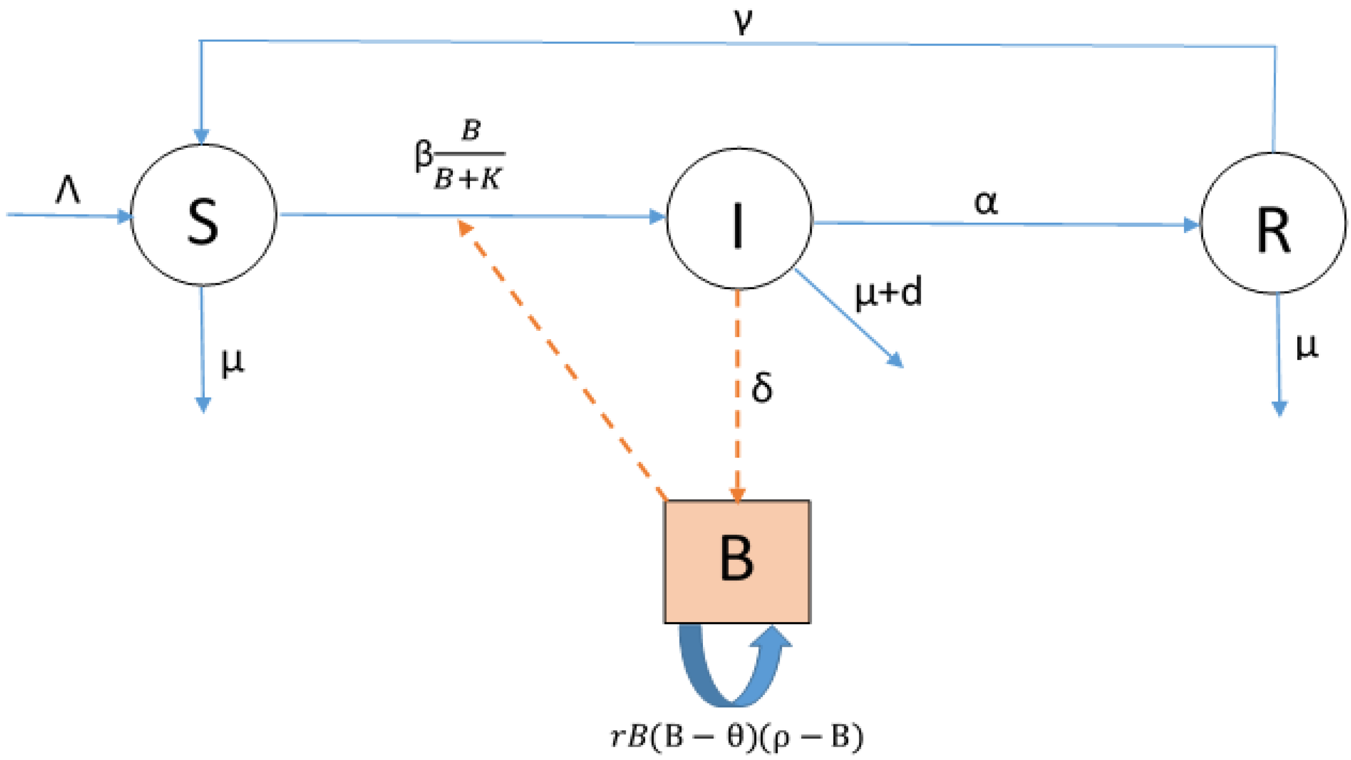
Figure 1. Graphical representation of proposed model of cholera dynamics.
Sustainability 15 10384 g001
Figure 2. Simulation of model (2) when Λ = 10 , β = 0.0001 and ϵ = 50 , 000 (so that θ ϵ = 9.5 × 10 5 , R 0 0 = 0.0103 , and ξ = 0.0495 ) using various initial conditions chosen in attraction domain of Q 0 . The remaining parameters are consistent with those listed in Table 1. Each subfigure corresponds to each state of model (2). (a) Susceptible. (b) Infected. (c) Recovered. (d) Bacteria.
Sustainability 15 10384 g002
Figure 3. Simulation of model (2) when Λ = 50 , β = 0.0015 , θ = 10 6 and ϵ = 50 , 000 (so that θ ϵ = 9.5 × 10 5 , ξ = 0.0495 , and R 0 0 = 0.7702 ) using various initial conditions ( S ( 0 ) , I ( 0 ) , R ( 0 ) , B ( 0 ) ) chosen in the domains D 1 = ] 0 ; 50 , 000 ] × ] 0 ; 10 ] × ] 0 ; 50 ] × 2 × 10 5 , 3 × 10 5 , 4 × 10 5 , 5 × 10 5 and D 2 = ] 0 ; 50 , 000 ] × ] 0 ; 10 ] × ] 0 ; 50 ] × 7.5 × 10 5 , 8 × 10 5 , 9 × 10 5 , 9.5 × 10 5 . The remaining parameters are consistent with those listed in Table 1. Each subfigure corresponds to each state of model (2). (a) Susceptible. (b) Infected. (c) Recovered. (d) Bacteria.
Sustainability 15 10384 g003
Figure 4. Simulation of model (2) when d = 0.7 , γ = 0.5 , α = 0.45 (so that R 0 0 = 0.0058 , ξ = 0.0505 and R 0 ( Q ρ ) = 0.0033 ) and initial conditions are chosen in D 3 = ] 0 ; 50 , 000 ] × ] 0 ; 10 ] × ] 0 ; 50 ] × 0.9 × 10 6 , 1.2 × 10 8 . The remaining parameters are consistent with those listed in Table 1. Each subfigure corresponds to each state of model (2). (a) Susceptible. (b) Infected. (c) Recovered. (d) Bacteria. (e) Zoom of bacteria graph.
Sustainability 15 10384 g004
Figure 5. Simulation of model (2) when Λ = 30 , β = 0.01 (so that R 0 0 = 3.0809 > 1 ) and various initial conditions have been taken in D 3 = ] 0 ; 7.5 × 10 6 ] × ] 0 ; 1.5 × 10 3 ] × ] 0 ; 7.5 × 10 3 ] × 0 , 1.5 × 10 8 . The remaining parameters are consistent with those listed in Table 1. Each subfigure corresponds to each state of model (2). (a) Susceptible. (b) Infected. (c) Recovered. (d) Bacteria. (e) Zoom of bacteria graph.
Sustainability 15 10384 g005
Figure 6. Simulation of model (2) when Λ = 50 , β = 0.02 and r = 10 20 (so that R 0 ( Q ρ ) = 0.0526 and R 0 0 = 1.7594 × 10 3 ) and various initial conditions in R + 4 . The remaining parameters are consistent with those listed in Table 1. Each subfigure corresponds to a specific state of model (2). (a) Infected, (b) Bacteria.
Sustainability 15 10384 g006
Figure 7. Simulation of model (2) when all parameters values are as in Table 1 (so that R 0 ( Q ρ ) = 0.0023 , R 0 0 = 0.0045 , ϵ = 50 , 000 and ξ = 0.0495 ) and various initial conditions chosen in D 3 = ] 0 ; 50 , 000 ] × ] 0 ; 10 ] × ] 0 ; 50 ] × 10 5 , 9.5 × 10 5 and in D 4 = ] 0 ; 50 , 000 ] × ] 0 ; 10 ] × ] 0 ; 50 ] × 10 6 , 2 × 10 8 . Each subfigure corresponds to a specific state of model (2). (a) Infected, (b) Bacteria, (c) Zoom on Bacteria population.
Sustainability 15 10384 g007
Figure 8. Simulation of model (2) when Λ = 30 , β = 0.001 and ϵ = 1000 (so that ξ = 0.0010 , R 0 ( Q ρ ) = 0.027 and R 0 0 = 0.308 ). The remaining parameters are consistent with those listed in Table 1. Various initial conditions chosen in D 5 = ] 0 ; 50 , 000 ] × ] 0 ; 10 ] × ] 0 ; 50 ] × 10 5 , 5 × 10 5 and D 6 = ] 0 ; 50 , 000 ] × ] 0 ; 10 ] × ] 0 ; 50 ] × 7 × 10 5 , 2 × 10 8 . Each subfigure corresponds to a specific state of model (2). (a) Infected, (b) Bacteria, (c) Zoom on Bacteria population.
Sustainability 15 10384 g008
Figure 9. Simulation of model (2) when β = 0.1 , μ = 1.04 × 10 3 , θ = 0.999 × 10 8 and ϵ = 50 , 000 (so that ξ = 5.005 × 10 8 , R 0 0 = 0.0104 and R 0 ( Q ρ ) = 4.5370 ). The remaining parameters are consistent with those listed in Table 1. Various initial conditions chosen in D 7 = ] 0 ; 50 , 000 ] × ] 0 ; 10 ] × ] 0 ; 50 ] × 10 5 , 2 × 10 8 . Each subfigure corresponds to the two following states of model (2): (a) Infected. (b) Bacteria.
Sustainability 15 10384 g009
Figure 10. Simulation of R 0 0 for various values of θ [ 0 ; 10 6 ] and ρ [ 10 6 ; 10 8 ] when r = 10 13 and the remaining parameters are consistent with those listed in Table 1.
Sustainability 15 10384 g010
Figure 12. Region of plane ( ρ , θ ) in which Q 0 and Q ρ are stable when r = 10 13 and the remaining parameters are consistent with those listed in Table 1. (a) For ϵ = 1 , (b) For ϵ = 50 , 000 .
Sustainability 15 10384 g012
Figure 13. Bifurcation Diagram of R 0 0 when (a) δ = 23 (b) λ = 20 and μ = 0.05 (c) λ = 20 , μ = 0.05 , and δ = 33 . Each of the three curves in each subfigure is associated with a specific solution of Equation (28).
Sustainability 15 10384 g013
Table 1. Numerical values for the parameters of model (2).
DefinitionSymbolEstimatedSource
Recruitment rate Λ 10 day 1 Assumed
Bacteria ingestion rate β 0.0001 person 1 day 1 Assumed
Human population death rate μ 0.0104 day 1 [13]
Bacteria shedding rate δ 70 cells/(mL day)[14]
Half-saturation constantK 10 7 cells/person/mL/dayAssumed
Cholera related deathd0.6 year 1 Assumed
Loss of immunity rate γ 0.01 day 1 Assumed
Recovery rate α 0.045 day 1 [15]
Growth rate of Vibriosr1 × 10 18 day 1 Assumed
Carrying capacity bacterial population ρ 1 × 10 8 cell/mLAssumed
Allee threshold bacterial population θ 1 × 10 6 cell/mLAssumed
Disclaimer/Publisher’s Note: The statements, opinions and data contained in all publications are solely those of the individual author(s) and contributor(s) and not of MDPI and/or the editor(s). MDPI and/or the editor(s) disclaim responsibility for any injury to people or property resulting from any ideas, methods, instructions or products referred to in the content.