Design of an Equipped Vehicle for In Situ Road Lighting Measurement

Abstract

Sustainable road lighting aims to minimize energy consumption and reduce carbon emissions. Road lighting assessment helps evaluate the energy efficiency of lighting systems, including the selection of appropriate lighting fixtures, efficient lamp technologies (such as LED), and lighting control strategies. Assessments can identify areas for improvement and guide the implementation of energy-saving measures. This study introduces a new technology that utilizes a specially equipped vehicle to efficiently and quickly measure photometric quantities on long, illuminated roads. The measurement ranges for illuminance and luminance are (0.1 to 1000) lx and (0.1 to 100) cd/m², respectively. The equipped vehicle has a positioning resolution of less than 1 cm. A sampling distance of less than 2 m while traveling at a speed of approximately 20 km/h and a sampling rate of 3 samples/s. To test the system’s applicability, the road used in this study was slightly sloped and curved. The results indicate a strong correlation between the illuminance distributions measured by the new method and those measured by traditional methods, thereby confirming the effectiveness of this innovative approach.

1. Introduction

Sustainability is a critical consideration for all industries, including the lighting industry. LED and smart lighting technologies have been proposed as potential solutions to improve energy efficiency, reduce carbon emissions, and achieve sustainability goals [1,2,3]. Smart lighting technology takes LED lighting a step further by incorporating sensors, controls, and connectivity to create a more efficient and sustainable lighting system. A study by the European Commission found that smart lighting systems could reduce energy consumption by up to 70% compared to traditional lighting systems [4,5]. The study also found that the implementation of smart lighting systems could lead to a reduction in carbon emissions of up to 500 million tons per year by 2030 [6,7]. LED and the Internet of Things have become essential solutions for the smart city. The development of dynamic lighting as the solution for intelligent cities automatically dims lighting under the right conditions [8,9]. Keeping the balance between energy savings and a safe lighting environment is the aim of intelligent lighting. The dynamic LED road lighting with a dimming controller can control the lighting levels according to traffic flow and weather conditions [10,11,12]. Increasing the lighting level helps car drivers have better visibility during rainy or foggy weather [13,14]. Decreasing the lighting level achieves energy savings during low traffic flow conditions. The high-efficiency road-lighting measurement system and the compatible standards help achieve a high-quality lighting environment for a smart city [15,16]. Road lighting assessments assist in evaluating the durability, reliability, and lifespan of lighting systems. By considering factors such as maintenance requirements, lamp longevity, and operational performance, sustainable lighting solutions can be selected that minimize waste generation, promote longevity, and reduce the need for frequent replacements.

The LED road lighting environment and luminaire specifications have to conform to international standards, and the safety of LED road lighting can be expected. The typical specifications of the LED luminaire include the luminance intensity distribution, correlated color temperature, spectrum, and luminance [17]. The optical parameters of the LED luminaire can be measured in an accredited laboratory. The specifications of the LED road-lighting environment include the illuminance distribution, luminance distribution, color distribution, uniformity, and Threshold Increment (TI) [18]. The supervision unit for road lighting has to do a random check to evaluate the initially established road lighting according to national or international standards. After the road lighting has been installed for a period of time, regular measurements are needed to assess the light decay and formulate the maintenance strategy for the new type of LED road lighting. In recent times, there has been an increasing interest in the development of new measurement systems to precisely assess the effectiveness of roadway lighting systems. These systems typically use objective measures, such as illuminance, luminance, or uniformity, to quantify the performance of the lighting system. Several road lighting evaluation systems have been widely accepted by lighting experts and have been utilized to assess the efficacy of roadway lighting systems across various environments [19,20,21,22].

The on-site evaluation of the LED road lighting environment is according to CIE 140:2019, CIE 194:2011, and EN 13201-2:2015 [23,24,25]. The quality characteristics of road lights are measured by illuminance and luminance, obtained in the field of calculation on the road. The positions of the field of calculation are according to CIE 140:2019. There are more than 60 points on a 60 m road, which is the spacing between two luminaires. It would take more than 30 min to obtain effectiveness by point-measurement in a 60 m road lighting environment. The Imaging Luminance Measurement Device (ILMD) and array-type illuminance measurement system were developed for measuring the road lighting environment. Although these systems reduce the measurement time by a few minutes, they need to block the road and implement traffic control during measurement. The vehicle-type road lighting measurement system, which mounts an illuminance meter on the back and front, is a highly efficient solution. The height of the vehicle caused the shadow. The illuminance on the road surface cannot be obtained with this system. We propose a new vehicle-type road lighting measurement system for high-efficiency road lighting evaluation [26,27]. The illuminance meters are mounted on the top of the vehicle to calculate the illuminance distribution on the road. An ILMD is placed on the car to measure the luminance distribution.

The Point Measurement method involves using a single illuminance meter and luminance to measure the characteristics of road lighting. According to the CIE 140:2019 standard, measurements can be taken at grid points between road lights. However, the main issue is that it takes at least 2 h to complete a 60 m road lighting measurement, as

Table 1. The typical methods for road lighting measurement.

Measurement Type	Point Measurement	Array-Type Measurement	Equipped Vehicle (Illuminance at the Vehicle Top)	Equipped Vehicle (Illuminance Calculated on the Road)
Methods of illuminance measurement	Point to point by an illuminance meter	3 illuminance meters	3 illuminance meters at the vehicle’s top	3 illuminance modules at the vehicle’s top
Measurement time 1	120 min	3 min	10 s	10 s
Position of illuminance distribution	Road surface	Road surface	Vehicle’s top	Road surface
Luminance distribution	Luminance meter	None	None	Calibrated ILMD 2
Field of view of luminance measurement	0.1° to 2° (overlapping issue)	None	None	Up to 0.01° (more than 100 pixels, no overlapping issue)

¹ The spacing between road lights set as 60 m. ² Image Luminance Measurement Device (ILMD).

.

The array-type measurement method utilizes three installed illuminance meters directly near the road surface to measure the road illuminance distribution automatically, complying with the CIE standards. The characteristics of array-type measurement method shown as Table 1.

The Equipped Vehicle measurement method can be divided into two categories. The first category involves directly measuring illuminance on the vehicle’s top. The second category involves analyzing the light intensity distribution of the road lights and calculating the road illuminance distribution based on that. The former method obtains the road illuminance distribution at the height of the vehicle’s roof or estimates the illuminance distribution on the road. However, under complex road lighting conditions, it is not possible to accurately calculate the road illuminance distribution as Table 1.

The latter method, which is the approach of this paper, involves analyzing the light intensity distribution of each road light using three sets of illuminance modules and calculating the road illuminance based on grid points, as Table 1.

2. The Illuminance Measurement and Calculation for LED Road Lighting

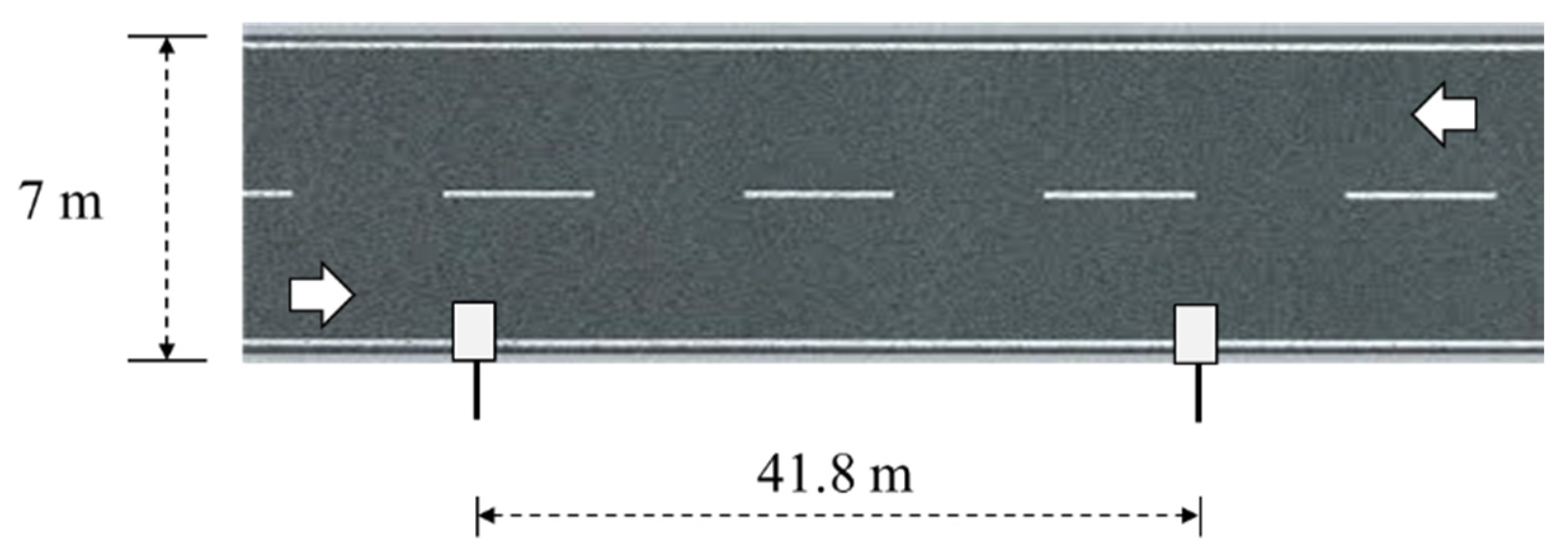
The on-site illuminance meter obtains the illuminance distribution according to CIE 140:2019. The suitable specification of the illuminance meter is 0.1 lx to 100 lx, which is applied for measuring the illuminance of the road surface. The position of calculation points along the longitudinal and transverse directions is relative to the lane width and the spacing of luminaires. The obtained illuminance distribution can be analyzed as the average illuminance, maximum and minimum illuminance, overall uniformity, and longitudinal uniformity. We established a road lighting experiment field to simulate highway conditions and evaluate the illuminance of various heights of luminaires. LED luminaires were mounted on the adjustable light poles, and the height, the light incident angle, and the length of the setting arm can be changed on the experiment field. The electrical power is 120 W, the luminous flux is 12,746 lm, and the luminous distribution type is semi-cut-off A. The spacing between these two luminaires is 41.8 m, and the lane width is 7 m. The luminaires were set at 0 m and 41.8 m, as shown in Figure 1. We set the height of the luminaires at 8 m, 10 m, and 12 m. We used the in-field array-type illuminance measurement system to measure the illuminance distribution according to CIE 140:2019, shown in Figure 2. The illuminance distribution for luminaires set at 8 m, 10 m, and 12 m heights was measured. We calculated the illuminance distribution at 10 m and 12 m by the Inverse Square Law of Illuminance based on the measurement result at 8 m height. The measurement and calculation results are shown in Figure 3. The maximum deviations between measurement and calculation at 10 m and 12 m are 45% and 62%, respectively. A significant variation happened in the two luminaires’ cross-field of light. If we directly measure the illuminance by the illuminance meter on the vehicle’s top and then calculate the illuminance by the Inverse Square Law of Illuminance, it would cause significant error results.

3. The Equipped Vehicle for Road Lighting Measurements

3.1. The Design of an Automatic Illuminance Measurement System for the Equipped Vehicle

The equipped vehicle was developed for in situ measurement of road lighting. An illustration of the equipped vehicle is shown in Figure 4. The equipped vehicle comprises three illuminance-meter modules, an Image Luminance Measurement Device (ILMD), and position measurement modules. The three illuminance-meter modules were set on the cross frame on the vehicle’s top. Each illuminance-meter module has four illuminance meters facing different directions: forward, backward, left, and up directions along the moving path, as shown in Figure 5. The illuminance-meter modules were set at 2 m in height. The distance between the center and edge illuminance-meter modules was 1.5 m. The encoder is mounted on the rear axle shaft. The gyro sensor is mounted in the middle of the frame on the vehicle’s top. The Inertial Measurement Unit (IMU) is integrated with the gyro sensor and encoder and calculates the accurate position when the equipped vehicle moves on the road. The connections between the above modules are shown in Figure 6. The combination of the resolution of the encoder per rotation and the perimeter of the tire will give a positioning resolution of less than 1 cm. The relative positions between the target luminaire and these illuminance meters are captured by the IMU. The captured irradiance and relative coordination analyze the luminance intensity of road lighting. The illuminance on the road’s surface can be used to calculate the luminance intensity distribution of road lighting. The uniformity of illuminance, the particular height of vertical illuminance, and horizontal illuminance can also be calculated.

The illuminance data are measured by the illuminance meters mounted on the equipped vehicle. The schematic diagram of the equipped vehicle for measuring road lighting is shown in Figure 7. The vectors of the illuminance meters $\stackrel{⃑}{S_{\mathrm{i}}}$ and road lights $\stackrel{⃑}{R_{\mathrm{j}}}$ were obtained by the IMU. The equation of illuminance can be expressed as follows:

$$\begin{gathered} E_{ai}=\frac{I_1·\mathrm{m}\mathrm{a}\mathrm{x}[{\widehat{n}}_{\mathrm{a}\_i}·\left({\stackrel{⃑}{R}}_1-{\stackrel{⃑}{S}}_{\mathrm{a}\_i}\right),0]}{{\left|{\stackrel{⃑}{R}}_1-{\stackrel{⃑}{S}}_{\mathrm{a}\_i}\right|}^3}+\frac{I_2·\mathrm{m}\mathrm{a}\mathrm{x}[{\widehat{n}}_{\mathrm{a}\_i}·\left({\stackrel{⃑}{R}}_2-{\stackrel{⃑}{S}}_{\mathrm{a}\_i}\right),0]}{{\left|{\stackrel{⃑}{R}}_2-{\stackrel{⃑}{S}}_{\mathrm{a}\_i}\right|}^3}+\frac{I_3·\mathrm{m}\mathrm{a}\mathrm{x}[{\widehat{n}}_{a\_\mathrm{i}}·\left({\stackrel{⃑}{R}}_3-{\stackrel{⃑}{S}}_{\mathrm{a}\_i}\right),0]}{{\left|{\stackrel{⃑}{R}}_3-{\stackrel{⃑}{S}}_{\mathrm{a}\_i}\right|}^3} \\ +\frac{I_4·\max \left[{\widehat{n}}_{\mathrm{a}\_i}·\left({\stackrel{⃑}{R}}_4-{\stackrel{⃑}{S}}_{\mathrm{a}\_i}\right),0\right]}{{\left|{\stackrel{⃑}{R}}_4-{\stackrel{⃑}{S}}_{\mathrm{a}\_i}\right|}^3} \end{gathered}$$

(1)

$$E_{bi}=\frac{I_2·\mathrm{m}\mathrm{a}\mathrm{x}[{\widehat{n}}_{\mathrm{b}\_i}·\left({\stackrel{⃑}{R}}_2-{\stackrel{⃑}{S}}_{\mathrm{b}\_i}\right),0]}{{\left|{\stackrel{⃑}{R}}_2-{\stackrel{⃑}{S}}_{\mathrm{b}\_i}\right|}^3}+\frac{I_4·\mathrm{m}\mathrm{a}\mathrm{x}[{\widehat{n}}_{\mathrm{b}\_i}·\left({\stackrel{⃑}{R}}_4-{\stackrel{⃑}{S}}_{\mathrm{b}\_i}\right),0]}{{\left|{\stackrel{⃑}{R}}_4-{\stackrel{⃑}{S}}_{\mathrm{b}\_i}\right|}^3}$$

(2)

$$E_{ci}=\frac{I_3·\mathrm{m}\mathrm{a}\mathrm{x}[{\widehat{n}}_{\mathrm{c}\_i}·\left({\stackrel{⃑}{R}}_3-{\stackrel{⃑}{S}}_{\mathrm{c}\_i}\right),0]}{{\left|{\stackrel{⃑}{R}}_3-{\stackrel{⃑}{S}}_{\mathrm{c}\_i}\right|}^3}+\frac{I_4·\mathrm{m}\mathrm{a}\mathrm{x}[{\widehat{n}}_{\mathrm{c}\_i}·\left({\stackrel{⃑}{R}}_4-{\stackrel{⃑}{S}}_{\mathrm{c}\_i}\right),0]}{{\left|{\stackrel{⃑}{R}}_4-{\stackrel{⃑}{S}}_{\mathrm{c}\_i}\right|}^3}$$

(3)

$$E_{di}=\frac{I_1·\mathrm{m}\mathrm{a}\mathrm{x}[{\widehat{n}}_{\mathrm{d}\_i}·\left({\stackrel{⃑}{R}}_1-{\stackrel{⃑}{S}}_{\mathrm{d}\_i}\right),0]}{{\left|{\stackrel{⃑}{R}}_1-{\stackrel{⃑}{S}}_{\mathrm{d}\_i}\right|}^3}+\frac{I_3·\mathrm{m}\mathrm{a}\mathrm{x}[{\widehat{n}}_{\mathrm{d}\_i}·\left({\stackrel{⃑}{R}}_3-{\stackrel{⃑}{S}}_{\mathrm{d}\_i}\right),0]}{{\left|{\stackrel{⃑}{R}}_3-{\stackrel{⃑}{S}}_{\mathrm{d}\_i}\right|}^3}$$

(4)

where ${\stackrel{⃑}{R}}_1\approx \left(\begin{array}{ccc}0& a& H\end{array}\right)$, ${\stackrel{⃑}{R}}_2\approx \left(\begin{array}{ccc}{W}_{\mathrm{T}}& a& H\end{array}\right)$, ${\stackrel{⃑}{R}}_3\approx \left(\begin{array}{ccc}d& W_{\mathrm{n}}·W_T+p-a& H\end{array}\right)$, ${\stackrel{⃑}{R}}_4\approx \left(\begin{array}{ccc}d+W_T& W_{\mathrm{n}}·W_{\mathrm{L}}+p-a& H\end{array}\right)$, W_T is the spacing between road lights (m), W_n is the number of the traffic lanes, N is the number of points in the longitudinal direction, H is the height of a road lighting (m), I is the luminous intensity (cd), a is the distance between the road edge and center of road lighting (m), p is the length of the road divider, W_L is the lane width (m), and d is the spacing between points in the longitudinal direction.

The luminance intensity distribution $I_i\left(\frac{{\stackrel{⃑}{R}}_j-{\stackrel{⃑}{S}}_i}{\left|{\stackrel{⃑}{R}}_j-{\stackrel{⃑}{S}}_i\right|}\right)$ of road lights is calculated by linear regression according to Equations (1)–(4). In this study, LabVIEW-based software was utilized to automate the measurement and analysis of various parameters, including the horizontal and vertical illuminance distributions and the flicker resulting from non-uniformity. The luminous intensity distributions of road lighting were used to compute these parameters. Notably, the aforementioned theories are applicable in the case of curved or sloped roads, as well as irregularly arranged road lighting.

3.2. The Design of an ILMD for Automatic Luminance Measurement for the Equipped Vehicle

The calibrated ILMD is mounted on the frame of the equipped vehicle, as shown in Figure 1. The specifications of the ILMD are as follows: the pixel number is 2488 × 2048 pixels, the dynamic range is 12 bits, the frame rate is 38 fps, and the 1.25 cm color CMOS image sensor. The high resolution and high dynamic range of the ILMD can provide a high sampling rate and in situ road lighting measurements. The ILMD was set up to measure the luminance distribution of the road. The LED was set at 1.5 m height according to CIE 140:2019. The equipped vehicle’s ILMD measurement system is composed of a calibrated camera and position measurement module. The camera captures the images when the car is moving. The calibration and correction files are applied to calculate the luminance and color distribution of each image. The software automatically provides the field of calibration positions from position data according to CIE 140:2019. Each region of interest is analyzed for luminance relative to road parameters. The measurement and analysis flow are shown in Figure 8. The camera has to correct the image sensor’s flat field for all focal lengths. The camera’s shutter speed, iris, and gain have to be calibrated and traced to the luminance standard. The color calibration of the camera is performed through the GretagMacbeth 24 ColorChecker in a light booth. The color standards are traced to the calibrated spectroradiometer. The calibration process and software of the ILMD are shown in Figure 9. Figure 9a was the setup of the calibration process for ILMD. Figure 9b shows that the ILMD was calibrated in various setting conditions, such as gain, exposure time, and aperture. The calibrated ILMD can provide accurate luminance and color distribution.

According to CIE 140:2019, the position of calculation points has to be set by the range finder. It would take about 30 min to measure the luminance distribution for a 50 m field of calculation. In general, the field of view of the luminance meter needs to be larger to distinguish each point in the field. We developed a road edge algorithm to automatically detect the relevant area’s edge, either the curve or the straight road, as shown in Figure 10. Compared to the typical luminance meter, the field of view is set at a specific angle, such as 0.1°, 1°, and 2°. It would cause an overlap area when using the typical luminance meter, according to CIE 140:2019. We can use the high-pixel number camera to measure the luminance distribution, and each position of the calibration point has more than 100 pixels, which is enough to calculate the luminance.

4. Measurement Results by the Equipped Vehicle

4.1. Measurement Results of Illuminance Distribution by the Equipped Vehicle

To verify the on-road measurement system, a road on campus was selected for measurement. The height of the light pole is 7.2 m, the distance between the light poles is 30 m, the width of the road is 3.5 m, the light pole is set on one roadside, there is no separation island on the road, and there is a shoulder width of 0.2 m, as shown in Figure 11. The experimental field has uphill and downhill sections and slight bends to verify the adaptability of the technology in various road environments. A mobile multi-channel automatic illuminance measurement system was used to compare the equipped vehicle. The experimental analysis has two parts: horizontal illuminance measurement at 2 m and horizontal illuminance on the road surface.

In Figure 12 and Figure 13, we can observe the horizontal illuminances that were measured and converted at a height of 2 m on the downhill and uphill sections. The figures also provide information about the crosswise distances from the lane edge, denoted as Line 3 (0.6 m), Line 2 (1.8 m), and Line 3 (3.0 m). To derive the luminous intensity distributions of the road lighting, we used the recorded illuminance distributions (E_ai, E_bi, E_ci, and E_di) along the road, which were described in the previous section. Based on our analysis, we found that the horizontal illuminances calculated from the luminous intensity distributions were consistent with the values obtained from measurements.

Figure 14 and Figure 15 show the experimental results of ground horizontal illuminance on the uphill and downhill sections. An array-type illuminance measurement system measured the illuminance distribution. The calculated illuminance distribution is based on the light intensity distribution of each road lighting, which is calculated by the equipped vehicle. The average and uniformity of the measured horizontal illuminance by an array-type illuminance measurement system on the uphill section are 24.8 lx and 0.39, respectively. The converted results are 24.7 lx and 0.39, respectively. For the downhill case, the average illuminance and uniformity were converted to 19.6 lx and 0.70, respectively. These values were found to be similar to the measured values of 19.9 lx and 0.72 obtained from the array-type illuminance measurement system. Furthermore, this method enables the calculation of other useful variables, such as the distribution of vertical illuminance at specific elevations and the flicker resulting from non-uniformity.

4.2. Measurement Results of Luminance Distribution by the Equipped Vehicle

The present study involved the simultaneous capture of luminance images and recorded illuminances. The sampling distance (m/sample) can be calculated from the speed of the vehicle (m/s) divided by the sampling rate (samples/s) of the measurement equipment. For example, an equipped vehicle with a speed of 20 km/h (or 5.6 m/s) will have a sampling distance of less than 2 m at a sampling rate of 3 samples/s of the equipment. The equipped-vehicle method for measuring road lighting can be significantly reduced compared to the traditional single-point measurement method. With a vehicle speed of 20 km/h, it is already safe to drive on regular roads. If a higher-speed measurement device is chosen, with a sampling rate of 10 samples/s and a sampling distance of 1.6 m/s, the speed of the equipped vehicle can be further increased to 60 km/h. Figure 16 illustrates a typical uphill image obtained using the ILMD. For each of the four measurements taken, with an average vehicle speed of approximately 11 km/h, images were captured at distances of 0 m, 7.4 m, 16.6 m, and 23.9 m from the starting point. A specific section of about 30 m (green trapezoidal box) is shown in Figure 16c. The yellow circles indicate that point sampling was performed automatically using the method described in the previous section, with an acceptance angle of 0.1°, as shown in Figure 17a. The distance from the closest position to the ILMD was 20.6 m, as shown in Figure 17a. The resulting luminance values were then plotted against the sampling position in Figure 17b. At a measurement distance of 20.6 m, the average luminance (L_ave) and uniformity (U₀) were found to be 1.14 cd/m² and 0.85, respectively.

Similarly, images were captured and processed for measuring distances between 27.9 m and 44.5 m, and the luminance values were obtained for the same sampling positions. The average luminance and uniformity were then plotted as a function of observation distance in Figure 18a,b, respectively. The results indicate that L_ave ranges from 1.12 to 1.23 cd/m², and U₀ ranges from 0.76 to 0.86. The variation in the average value was found to be 9.7%, independent of the observation distance. Therefore, the reflected luminance variation is small for this illuminated road.

5. Discussion

For the equipped vehicle for illuminance distribution measurement, 9 illuminance meters were another option. Each illuminance meter module has 3 illuminance meters that have been set in the upward, forward, and left directions. The schematic diagram for a 9-illuminance-meter type of equipped vehicle is shown in Figure 7. The equation of illuminance can be expressed as follows:

$$E_{ai}=\frac{I_1·\mathrm{m}\mathrm{a}\mathrm{x}[{\widehat{n}}_{\mathrm{a}\_i}·\left({\stackrel{⃑}{R}}_1-{\stackrel{⃑}{S}}_{\mathrm{a}\_i}\right),0]}{{\left|{\stackrel{⃑}{R}}_1-{\stackrel{⃑}{S}}_{\mathrm{a}\_i}\right|}^3}+\frac{I_2·\mathrm{m}\mathrm{a}\mathrm{x}[{\widehat{n}}_{\mathrm{a}\_i}·\left({\stackrel{⃑}{R}}_2-{\stackrel{⃑}{S}}_{\mathrm{a}\_i}\right),0]}{{\left|{\stackrel{⃑}{R}}_2-{\stackrel{⃑}{S}}_{\mathrm{a}\_i}\right|}^3}+\frac{I_3·\mathrm{m}\mathrm{a}\mathrm{x}[{\widehat{n}}_{a\_\mathrm{i}}·\left({\stackrel{⃑}{R}}_3-{\stackrel{⃑}{S}}_{\mathrm{a}\_i}\right),0]}{{\left|{\stackrel{⃑}{R}}_3-{\stackrel{⃑}{S}}_{\mathrm{a}\_i}\right|}^3}$$

(5)

$$E_{bi}=\frac{I_2·\mathrm{m}\mathrm{a}\mathrm{x}[{\widehat{n}}_{\mathrm{b}\_i}·\left({\stackrel{⃑}{R}}_2-{\stackrel{⃑}{S}}_{\mathrm{b}\_i}\right),0]}{{\left|{\stackrel{⃑}{R}}_3-{\stackrel{⃑}{S}}_{\mathrm{b}\_i}\right|}^3}+\frac{I_3·\mathrm{m}\mathrm{a}\mathrm{x}[{\widehat{n}}_{\mathrm{b}\_i}·\left({\stackrel{⃑}{R}}_3-{\stackrel{⃑}{S}}_{\mathrm{b}\_i}\right),0]}{{\left|{\stackrel{⃑}{R}}_3-{\stackrel{⃑}{S}}_{\mathrm{b}\_i}\right|}^3}$$

(6)

$$E_{ci}=\frac{I_3·\mathrm{m}\mathrm{a}\mathrm{x}[{\widehat{n}}_{\mathrm{c}\_i}·\left({\stackrel{⃑}{R}}_3-{\stackrel{⃑}{S}}_{\mathrm{c}\_i}\right),0]}{{\left|{\stackrel{⃑}{R}}_3-{\stackrel{⃑}{S}}_{\mathrm{c}\_i}\right|}^3}$$

(7)

where ${\stackrel{⃑}{R}}_1\approx \left(\begin{array}{ccc}0& a& H\end{array}\right)$, ${\stackrel{⃑}{R}}_2\approx \left(\begin{array}{ccc}{W}_{\mathrm{T}}& a& H\end{array}\right)$, ${\stackrel{⃑}{R}}_3\approx \left(\begin{array}{ccc}d& W_n·W_T+p-a& H\end{array}\right)$, W_T is the spacing between road lights (m), W_n is the number of the traffic lanes, N is the number of points in the longitudinal direction, H is the height of a road lighting (m), I is the luminous intensity (cd), a is the distance between the road edge and center of road lighting (m), p is the length of the road divider (m), W_L is the lane width (m), and d is the spacing between points in the longitudinal direction (m).

The luminance intensity distribution $I_i\left(\frac{{\stackrel{⃑}{R}}_j-{\stackrel{⃑}{S}}_i}{\left|{\stackrel{⃑}{R}}_j-{\stackrel{⃑}{S}}_i\right|}\right)$ of road lights is calculated by linear regression according to Equations (5)–(7).

The recorded illuminance distribution in the upward and left directions can be used to calculate the spacing between road lights. The backward and forward directions can be used to calculate the spacing between road lights of opposite roads. We can use the equipped vehicle to measure the ground illuminance distribution automatically.

It is important to highlight the significance of the findings and the implications of the use of mobile systems for road lighting evaluation. The use of the equipped vehicle for road lighting measurement systems offers several advantages over traditional evaluation methods, such as a more comprehensive evaluation that can cover a larger area quickly and efficiently. This can lead to improved safety for drivers and pedestrians by identifying areas where the lighting is inadequate or uneven.

Another significant advantage of the equipped vehicle is its ability to monitor the performance of the outdoor lighting environment and individual lighting fixtures. This can help identify malfunctioning fixtures more quickly, reducing maintenance costs, improving the overall performance of the road lighting system, and reaching a sustainable city. In addition, the equipped vehicle can provide more accurate and consistent data by using calibrated measurement systems and ILMDs, which can help inform decision-making in the maintenance and upgrading of roadway lighting infrastructure.

However, there are also challenges associated with using the equipped vehicle, such as ensuring the accuracy and consistency of the collected data. It is essential to ensure that the measurement systems and ILMDs are calibrated correctly and that the data collected is reliable and consistent across different locations and times. Data processing and analysis can also be time-consuming and require specialized expertise, which may limit the widespread adoption of mobile systems for road lighting evaluation.

It is important to address these challenges and continue to develop and refine the use of the equipped vehicle for road lighting evaluation. The benefits of this approach can have a significant impact on transportation safety and infrastructure maintenance, and continued improvements in technology and data analysis can help overcome the challenges associated with this approach.

6. Conclusions

A vehicle equipped with a system for efficient and rapid measurements of illuminance and luminance along a lighted road was developed and evaluated. The measurement ranges for illuminance and luminance were (0.1 to 1000) lx and (0.1 to 100) cd/m², respectively, with a resolution of 0.3 m and a sampling distance of less than 2 m. The validity of the method was confirmed by comparing the illuminance distributions obtained by this method with those obtained by conventional methods. The equipped vehicle is suitable for evaluating long, well-lit roads, and the method can provide accurate and reliable results.

Road lighting assessment is an essential component of sustainable lighting practices. It helps align road lighting systems with environmental, economic, and social sustainability goals by optimizing energy efficiency, reducing environmental impact, ensuring safety, and supporting long-term planning. By incorporating sustainability principles into road lighting assessments, we can create more sustainable and resilient transportation infrastructure.

The use of the equipped vehicle for road lighting evaluation represents an important development in the field of transportation safety and infrastructure maintenance. Despite the challenges, the benefits of this approach can lead to a safer and more reliable transportation system, highlighting the importance of continued research and development in this area.

References

- Ramirez Lopez, L.J.; Grijalba Castro, A.I. Sustainability and Resilience in Smart City Planning: A Review. Sustainability 2021, 13, 181. [Google Scholar] [CrossRef]
- Girardi, P.; Temporelli, A. Smartainability: A methodology for assessing the sustainability of the smart city. Energy Procedia 2017, 111, 810–816. [Google Scholar] [CrossRef]
- Maria, T.A.; Niamh, M. The Concept of Sustainability in Smart City Definitions. Front. Built Environ. 2020, 6, 77. [Google Scholar] [CrossRef]
- Ayan, O.; Turkay, B. IoT-based energy efficiency in smart homes by smart lighting solutions. In Proceedings of the 2020 21st International Symposium on Electrical Apparatus & Technologies (SIELA), Bourgas, Bulgaria, 3–6 June 2020; pp. 1–5. [Google Scholar] [CrossRef]
- Shahzad, G.; Yang, H.; Ahmad, A.W.; Lee, C. Energy-efficient intelligent street lighting system using traffic-adaptive control. IEEE Sens. J. 2016, 16, 5397–5405. [Google Scholar] [CrossRef]
- Alam, M.R.; Reaz, M.B.I.; Ali, M.A.M. A Review of Smart Homes—Past, Present, and Future. IEEE Trans. Syst. Man Cybern. Part C Appl. Rev. 2012, 42, 1190–1203. [Google Scholar] [CrossRef]
- Hong, W.; Rahmat, B.N.N.N. Energy consumption, CO2 emissions and electricity costs of lighting for commercial buildings in Southeast Asia. Sci. Rep. 2022, 12, 13805. [Google Scholar] [CrossRef] [PubMed]
- Daely, P.T.; Reda, H.T.; Satrya, G.B.; Kim, J.W.; Shin, S.Y. Design of smart LED streetlight system for smart city with web-based management system. IEEE Sens. J. 2017, 17, 6100–6110. [Google Scholar] [CrossRef]
- Chen, Z.; Sivaparthipan, C.B.; Muthu, B. IoT based smart and intelligent smart city energy optimization. Sustain. Energy Technol. Assess. 2022, 49, 101724. [Google Scholar] [CrossRef]
- Kompier, M.E.; Smolders, K.C.; De Kort, Y.A. A systematic literature review on the rationale for and effects of dynamic light scenarios. Build. Environ. 2020, 186, 107326. [Google Scholar] [CrossRef]
- Wojnicki, I.; Kotulski, L. Empirical study of how traffic intensity detector parameters influence dynamic street lighting energy consumption: A case study in Krakow, Poland. Sustainability 2018, 10, 1221. [Google Scholar] [CrossRef] [Green Version]
- Bachanek, K.H.; Tundys, B.; Wiśniewski, T.; Puzio, E.; Maroušková, A. Intelligent street lighting in a smart city concepts—A direction to energy saving in cities: An overview and case study. Energies 2021, 14, 3018. [Google Scholar] [CrossRef]
- Jia, G.; Han, G.; Li, A.; Du, J. SSL: Smart Street Lamp Based on Fog Computing for Smarter Cities. IEEE Trans. Ind. Inform. 2018, 14, 4995–5004. [Google Scholar] [CrossRef]
- Ning, Z.; Huang, J.; Wang, X. Vehicular fog computing: Enabling real-time traffic management for smart cities. IEEE Wirel. Commun. 2019, 26, 87–93. [Google Scholar] [CrossRef]
- Mallapuram, S.; Ngwum, N.; Yuan, F.; Lu, C.; Yu, W. Smart city: The state of the art, datasets, and evaluation platforms. In Proceedings of the 2017 IEEE/ACIS 16th International Conference on Computer and Information Science, Wuhan, China, 24–26 May 2017; pp. 447–452. [Google Scholar] [CrossRef]
- Zubizarreta, I.; Seravalli, A.; Arrizabalaga, S. Smart city concept: What it is and what it should be. J. Urban Plan. Dev. 2016, 142, 04015005. [Google Scholar] [CrossRef]
- Mohan, D. Road safety in less-motorized environments: Future concerns. Int. J. Epidemiol. 2002, 31, 527–532. [Google Scholar] [CrossRef] [PubMed] [Green Version]
- Bhagavathula, R.; Gibbons, R.B.; Edwards, C.J. Relationship between roadway illuminance level and nighttime rural intersection safety. Transp. Res. Rec. 2015, 2485, 8–15. [Google Scholar] [CrossRef]
- Zhou, H.; Hsu, P.; Lin, P. A New Method to Evaluate Roadway Lighting Systems and Its Safety Effects. In Proceedings of the ITE 2010 Annual Meeting and Exhibit, Vancouver, BC, Canada, 8–11 August 2010; pp. 8–11. [Google Scholar]
- Greffier, F.; Muzet, V.; Boucher, V.; Fournela, F.; Dronneau, R. Use of an imaging luminance measuring device to evaluate road lighting performance at different angles of observation. In Proceedings of the 29th Quadrennial Session of the CIE, Washington, DC, USA, 14–22 June 2019; pp. 553–562. [Google Scholar] [CrossRef]
- Tomczuk, P.; Chrzanowicz, M.; Jaskowski, P.; Budzynski, M. Evaluation of street lighting efficiency using a mobile measurement system. Energies 2021, 14, 3872. [Google Scholar] [CrossRef]
- Gibbons, R.B.; Meyer, J. Development of a Mobile Measurement System for Roadway Lighting; National Surface Transportation Safety Center for Excellence: Blacksberg, VA, USA, 2018; p. 33. [Google Scholar]
- CIE 140:2019; Road Lighting Calculations. CIE: Vienna, Austria, 2000.
- CIE 194:2011; On Site Measurement of the Photometric Properties of Road and Tunnel Lighting. CIE: Vienna, Austria, 2011.
- EN 13201-2:2015; Road Lighting Performance Requirements. CEN: Brussels, Belgium, 2015.
- Hsu, S.W.; Chen, C.H.; Wu, K.N.; Hung, S.T. Colorimetric properties of LED illuminated roads studied by in-field measurements and simulations. In Proceedings of the 4th CIE Expert Symposium on Colour and Visual Appearance, Prague, Czech Republic, 6–7 September 2016; pp. 135–136. [Google Scholar]
- Hsu, S.W.; Wu, K.N.; Hung, S.T. Performance of LED road lightings studied by detailed in-field measurements with various devices. In Proceedings of the 28th Quadrennial Session of the CIE, Manchester, UK, 28 June–4 July 2015; pp. 590–591. [Google Scholar]
Figure 1.
The illustration of the road lighting in the experiment field.
Figure 2.
The in-field array-type illuminance measurement system: (a) the practical measurement in the experiment field; (b) the illustration of an array-type illuminance measurement system.
Figure 3.
The illustration of the road lighting on the experiment field: (a) the luminaires were set at 10 m height; (b) the luminaires were set at 12 m height.
Figure 4.
The illustration of the equipped vehicle: (a) isometric projection; (b) top view.
Figure 5.
The schematic diagram of the illuminance-meter module: (a) three-dimensional computer-aided design; (b) diagram of illuminance-meter modules.
Figure 6.
Connections between the modules on the equipped vehicle.
Figure 7.
The schematic diagram of the equipped vehicle for measuring road lighting.
Figure 8.
The measurement flow of the equipped ILMD on the equipped vehicle for measuring luminance and color distribution of road lighting.
Figure 9.
The calibration process and software for the camera: (a) the color calibration process; (b) the software applied for the calibration and correction files during the measuring.
Figure 10.
The edge detection algorithm analyzed the position of calibration points for calculating the luminance distribution of the road: (a) the straight road; (b) the curved road.
Figure 11.
The equipped vehicle was used to conduct experiments on a road.
Figure 12.
The horizontal illuminances at 2 m height measured by illuminance meters and converted by the equipped vehicle for a downhill lane: (a) line 1; (b) line 2; (c) line 3.
Figure 13.
The horizontal illuminances at 2 m height measured by illuminance meters and converted by the equipped vehicle for an uphill lane: (a) line 1; (b) line 2; (c) line 3.
Figure 14.
The horizontal illuminances near ground measured by near-ground illuminance meters and converted by the equipped vehicle for a downhill lane: (a) line 1; (b) line 2; (c) line 3.
Figure 15.
The horizontal illuminances near ground measured by near-ground illuminance meters and converted by the equipped vehicle for an uphill lane: (a) line 1; (b) line 2; (c) line 3.
Figure 16.
The luminance image was measured at various distances: (a) 0 m; (b) 7.4 m; (c) 16.6 m; (d) measurement distance is 23.9 m, and the region of interest is within the green frame.
Figure 17.
The measured luminance image by the ILMD: (a) sampling points of region of interest; (b) luminance distribution of all sampling points.
Figure 18.
The analyzed luminance results in various measurement distances: (a) average luminance; (b) uniformity as functions of measurement distance.