Abstract
The determination of soil parameters in geotechnical engineering and their variations during the construction process have long been a focal point for engineering designers. While the artificial neural network (ANN) has been employed for back analysis of soil parameters, its application to caisson sinking processes remains limited. This study focuses on the Nanjing Longtan Yangtze River Bridge project, specifically the south anchoring of an ultra-large rectangular caisson. A comprehensive analysis of the sinking process was conducted using 400 finite element method (FEM) models to obtain the structural stress and earth pressure at key locations. Multiple combinations of soil parameters were considered, resulting in a diverse set of simulation results. These results were then utilized as training samples to develop a back-propagating artificial neural network (BP ANN), which utilized the structural stress and earth pressure as input sets and the soil parameters as output sets. The BP ANN was individually trained for each stage of the sinking process. Subsequently, the trained ANN was employed to predict the soil parameters under different working conditions based on actual monitoring data from engineering projects. The obtained soil parameter variations were further analyzed, leading to the following conclusions: (1) The soil parameters estimated by the ANN exhibited strong agreement with the original values from the geological survey report, validating their reliability; (2) The surrounding soil during the caisson sinking exhibited three distinct states: a stable state prior to the arrival of the cutting edges, a strengthened state upon the arrival of the cutting edges, and a disturbed state after the passage of the cutting edges; (3) In the stable state, the soil parameters closely resembled the original values, whereas in the strengthened state, the soil strength and stiffness significantly increased, while the Poisson’s ratio decreased. In the disturbed state, the soil strength and stiffness were slightly lower than the original values. This study represents a valuable exploration of back analysis for caisson engineering. The findings provide important insights for similar engineering design and construction projects.
1. Introduction
The natural geotechnical parameters exhibit significant randomness and fuzziness, rendering geotechnical engineering a highly complex and nonlinear system [1,2,3]. Consequently, the issue of parameter uncertainty has become a bottleneck in theoretical analysis and numerical simulation of geotechnical mechanics. Obtaining accurate mechanical parameters of rock and earth masses through simple and feasible methods has thus emerged as a focal point in current geotechnical research [4,5]. The utilization of back analysis based on engineering monitoring results offers a solution to this problem. However, traditional methods have failed to effectively address optimization, resulting in low efficiency and complexity that hinder their widespread application in engineering. Therefore, with the rapid development of computer technology and intelligent algorithms, various neural networks and their improved models are gradually being employed for back analysis of geotechnical engineering parameters [6,7,8].
In recent years, significant achievements have been made in the application of intelligent algorithms for back analysis and prediction of structural bearing capacity and deformation in geotechnical engineering. In the context of large-volume concrete dams and earth-rockfill dams, mature ANN algorithms have been employed to train a large amount of experimental or numerical simulation data. The resulting models are commonly used for back analysis of dam material seepage characteristics [6], geotechnical parameters of the dam body and surrounding rock mass, as well as parameter variation during construction [9], and prediction of optimal dam arch shape [4]. During this period, the intelligent models used for prediction have also been continuously improving. Intelligent algorithms combining ANN with evolutionary algorithms [1], ANN combined with support vector machines [10], HS-BPNN algorithm combining backpropagation artificial neural network with harmony search algorithm [11], composite algorithms combining modified genetic algorithm and radial basis function neural networks (RBFNN) [12], BP ANN incorporating autoregressive integrated moving average model [13], and kernel extreme learning machine (KELM)-based response surface model (RSM) [14], have all been utilized for parameter back analysis of dams.
In terms of pile foundation, A variety of ANN models have been used to predict the bearing capacity of single pile [15] and the displacement of pile top [16]. Ismail, A. developed a robust hybrid training algorithm by combining particle swarm optimization (PSO) and BP algorithms [17]. Harandizadeh presented an application of two improved adaptive neuro-fuzzy inference system (ANFIS) techniques to estimate ultimate piles bearing capacity [18]. Subsequently, feedforward neural network (FFNN), radial basis functions neural networks (RBNN), general regression neural network (GRNN), and adaptive neuro-fuzzy inference system (ANFIS) were used to estimate the pullout forces [19].
In the field of tunnels, intelligent algorithms are commonly employed to determine geometric dimensions, constitutive relationships, material parameters, and boundary loading conditions [20]. Various methods have been employed, including the direct optimization method based on the genetic algorithm and the improved support vector regression algorithm (GA-SVR) [7], a novel evolutionary neural network based on immunized evolutionary programming [21,22], a new neural network based on the black hole algorithm [23], and the utilization of particle swarm optimization (PSO) to optimize extreme learning machine (ELM) [24].
Intelligent algorithms have not only been extensively applied in the analysis and prediction of parameters in dam, pile foundation, and tunnel engineering, but also have seen limited research in slope engineering, ground reinforcement, and foundation scour. Dai, Y. proposed a novel landslide warning method based on DBA-LSTM (displacement back analysis based on long short-term memory networks) [25]. The particle swarm optimization (PSO) algorithm [26] and the ANN optimized by the colonial competitive algorithm (ANN-ICA) [27] have been utilized for the analysis of soil strength or ground deformation [28]. Additionally, a combination of two ANN models, namely feed-forward backpropagation (FFBP) and radial basis function (RBF), was employed to predict the depth of bridge pile scour holes [5].
Although intelligent algorithms, primarily based on various types of ANNs, have made significant advancements in parameter back analysis and prediction in geotechnical engineering, most of the research has focused on dams, piles, and tunnels, with limited studies on other forms of foundation engineering. Applications in caisson and similar foundation forms are very rare. Moreover, intelligent parameter analysis is well-suited for studying the spatiotemporal variations of geotechnical and structural parameters during the construction process, particularly for foundation forms such as caissons, which experience significant ground disturbance and dynamic displacements. However, previous research has paid little attention to the patterns of parameter variations. Therefore, based on the ultra-large rectangular caisson foundation of the Longtan Yangtze River Bridge south anchorage in Nanjing, this study utilizes multiple sets of numerical simulation results to train a BP ANN model and conduct back analysis to determine the variations of surrounding soil parameters during the caisson sinking process.
2. Soil Parameter Back Analysis Method
2.1. Back Analysis Process
The main idea for using BP artificial neural network (BP ANN) in the back analysis of soil parameters around a caisson is to establish a correspondence between multiple sets of soil parameters and stress responses of the caisson structure by means of the finite element method (FEM). The ANN model is then trained using this correspondence data. Finally, the predicted soil parameters are obtained by inputting actual measured stress of the caisson into the model.
However, there are two difficulties in the analysis process. Firstly, the construction of the caisson differs from the general building process. As the internal soil is continuously excavated, the structure is always in a dynamic settling state, and the vertical displacement is very large. Surrounding soil may be disturbed and mechanical parameters may change. Thus, in order to reflect the evolution of soil parameters in each stage of settlement, it is necessary to divide the settling process into multiple working conditions and build an ANN model for each condition. Secondly, following the establishment of various working conditions, it is imperative to compute multiple FEM results for each condition, leading to a notable escalation in computational workload. Therefore, to minimize the number of FEM models without affecting the prediction accuracy, the uniform design method is used in this study to design the combination of soil parameters for each working condition. This ensures the representativeness of the soil parameters in each model and saves considerable computational load. Furthermore, a FEM parameterization modeling method is used to automatically iterate preprocessing, calculation, and post-processing based on the uniform design table, greatly improving simulation efficiency.
Figure 1 shows the seven steps of the back analysis. Step 1: Construct a uniform design table based on caisson information; Step 2: Establish soil parameter combinations based on the uniform design table and the reasonable distribution range of soil parameters; Step 3: Obtain the stress response of the caisson structure through the FEM model; Steps 4 and 5: Use the stress response obtained in Step 3 as the input set, and use the soil parameter combinations obtained in Step 2 as the output set to train the ANN models; Step 6: Process the measured stress data of the caisson, reduce its fluctuation, and select the measured data set corresponding to each simulation condition; Step 7: Input the measured data set into the ANN models to obtain the predicted soil parameters.

Figure 1.
Flow chart of soil parameter back analysis.
2.2. Uniform Design
The uniform design method is a novel statistical method to experimental design, based on number theory and multivariate statistical theory. It is particularly suited to dealing with complex scientific research topics involving multiple factors and levels and allows for more efficient completion of experimentation with fewer experiments. By contrast to traditional orthogonal design method, the uniform design prioritizes the uniform dispersion of experiment points across the parameters, rather than strict comparability of parameters. The goal is to ensure that each experiment is fully representative of a certain aspect, without imposing stringent controls on independent variables. The uniform design is facilitated through the use of a design table constructed using the good lattice point method, which involves the following steps:
(1) Identify an integer h that is smaller than a given experiment number n, such that the greatest common divisor of n and h is 1. The set of positive integers satisfying these conditions forms a vector h = (h1, …, hm);
(2) The elements of the uniform design table, uij, can be determined using the Equation (1):
where [mod n] denotes congruence, and if jhi is greater than n, it should be reduced by a suitable multiple of n so that the result lies within [1, n]. The uij values can be recursively computed using Equations (2) and (3).
2.3. BP ANN
The BP ANN represents a kind of classic multi-layer ANN composed of the input layer, hidden layer, and the output layer, each of which is fully interconnected. No interconnection exists between units of the same layer. The output value of each node in a layer is determined by the input from the previous layer and its excitation function and threshold.
During training, the network receives pairs of samples, and the activation values of the neurons propagate from the input layer through the hidden layer to the output layer, resulting in the final network output response value. The deviation between the actual output value and the expected value for the sample is utilized to estimate layer-specific errors, with subsequent error estimation extending successively to each preceding layer. The connection weight is corrected layer-by-layer from the output layer through each intermediate layer, all the way to the input layer, in a process of error backward propagation. This algorithm is known as the error backpropagation algorithm. The addition of an intermediate hidden layer and corresponding learning rules in BP algorithm confers the ability to recognize nonlinear patterns. The typical BP network contains three layers, each of which is fully connected, as depicted in Figure 2.

Figure 2.
BP ANN structure diagram.
Figure 2 shows the BP ANN structure where n represents the total number of nodes in the input layer, p denotes the number of nodes in the middle layer, and q denotes the number of nodes in the output layer. The input information is represented by “x1, …, xn”. wji refers to the weight from the ith input layer node to the jth hidden layer node. zj denotes the information acquired by the jth node of the hidden layer from the input layer and is obtained by Equation (4). Similarly, vkj represents the weight from the jth hidden layer node to the kth output layer node. The output information is designated by “y1, …, yn” and is derived using Equation (5).
f(net) is the node excitation function, as shown in Equation (6). In this study, sigmoid function, which is relatively common, is used as the excitation function.
3. South Anchoring Caisson Foundation of Longtan Yangtze River Bridge
3.1. Description of the Project
The Longtan Yangtze River Bridge, located at the conflux of Nanjing City and Zhenjiang City, Jiangsu Province, China, is a highway suspension bridge, constructed in compliance with the standard of six-lane highways in both directions. It has a total length of 4963 m, with a main span of 1560 m, ranking as the world’s ninth-largest span. This bridge’s south anchorage utilizes a rectangular caisson foundation that is 50 m high, divided into nine segments, with the first segment utilizing steel shell concrete and the remaining ones with a reinforced concrete structure.
Figure 3 and Figure 4 exhibit the caisson sinking and design diagram, with each segment of the caisson measuring 73.4 m in length and 56.6 m in width, except the first segment, which measures 73.8 m in length and 57.0 m in width. The partition wall in the first segment measures 1.4 m in thickness, whereas the remaining segments have partition walls of 2.0 m in thickness. A total of 30 rectangular holes (8.8 m × 9.8 m) are distributed within the caisson. Once the foundation was sunk into its designated location, the base was sealed with plain concrete. Then, concrete (15 back toe holes) and water (15 front toe holes) were poured into the hole, after which the caisson was capped with reinforced concrete.

Figure 3.
Sinking of the caisson.

Figure 4.
Anchorage and the foundation.
During the caisson construction, it was divided into three pouring processes and three sinking processes. In the first pouring process, 1~3 segments were constructed (20 m in height) and the caisson will sink 12.5 m with the water in the caisson being pumped out. In the second pouring process, 4~6 segments were constructed (15 m in height) and the caisson sunk 18.0 m without drainage. In the last pouring process, 7~9 segments were constructed (15 m in height) and the caisson sunk 19.5 m without drainage. Only after the capping concrete hardened was the upper anchor body constructed.
3.2. Monitoring Content
The field monitoring of the caisson involves a wide range of content, which serves as both a direct basis for the back analysis of soil parameters and as the primary content for post-processing of FEM models. Therefore, the quality of monitoring is crucial to the back analysis results. This study focuses on the monitoring content that may reflect the values and changes in the surrounding soil parameters, including the vertical soil pressure at the cutting edges and partition walls, the horizontal soil pressure of the shaft walls, and the vertical and horizontal shell stress at the cutting edges and partition walls. All sensors collect data every 4 h and upload it to the cloud-based visualization monitoring system.
Sixteen vertical soil pressure gauges were installed at the bottom of the cutting edges and four at the bottom of the partition walls. Figure 5a,b, respectively, show the distribution and installation position of sensors at the bottom of the caisson. The soil pressure at this position is the most intuitive reflection of the soil parameters in the layer where the cutting edges is located. Some studies indicate that, the greater the soil strength, the greater the pressure required to cut the soil at the cutting edges, resulting in larger soil pressure at the bottom of the caisson. Therefore, the monitoring data of earth pressure can be used for back analysis.
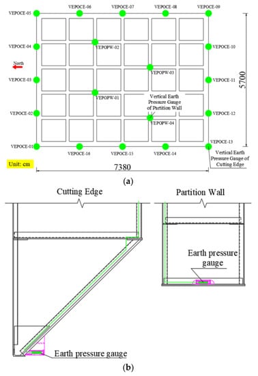
Figure 5.
Monitoring of earth pressure at the bottom of the caisson: (a) distribution of pressure gauges; (b) installation position of pressure gauges.
Fifty horizontal earth pressure gauges were installed on the shaft walls of the first, third, fourth, and ninth segment of the caisson. The layout plan and top view plan of sensors are shown in Figure 6a,b, respectively. The empirical calculation equation for the commonly used static earth pressures coefficient k0 is shown in Equation (7) [29]. It can be seen that k0 is related to the internal friction angle of the surrounding soil, so earth pressures on the shaft walls may be related to the surrounding soil parameters. It is the reason the earth pressures can be used for back analysis.


Figure 6.
Layout of earth pressure gauges on the shaft walls of the caisson: (a) top view; (b) front view.
Figure 6.
Layout of earth pressure gauges on the shaft walls of the caisson: (a) top view; (b) front view.
Eight vertical steel plate stress gauges and six horizontal steel plate stress gauges were installed at the bottom of the cutting edges, and 13 horizontal steel plate stress gauges were installed at the bottom of the partition walls. The layout plan and top view plan of sensors are shown in Figure 7a,b, respectively. The function of the bottom steel plate stress gauges is similar to that of the bottom earth pressure gauges. However, due to the spatial variability of soil parameters and construction disturbances, the values of earth pressure gauges fluctuate greatly, while the values of steel plate stress gauges are relatively stable. Therefore, the steel stresses are still used for the back analysis.

Figure 7.
Layout of steel plate stress gauges at the bottom of the caisson: (a) top view; (b) front view.
3.3. Geological Information
The location of the caisson is in an open area near the Yangtze River, with a relatively high groundwater level. The caisson has a depth of 50 m and involves five main soil and rock layers. From top to bottom, these layers are muddy silty clay, silty clay with silt, silty sand, medium-coarse sand, and moderately weathered silty mudstone. Within the caisson area, the thickness of each layer varies insignificantly. The geological profile is shown in Figure 8. The medium-coarse sand layer exhibits suitable strength, stiffness, and burial depth, making it the load-bearing layer for the caisson. The physical and mechanical properties of each layer are provided in Table 1, as indicated in the geological survey report.

Figure 8.
Geological plane.

Table 1.
Physical and mechanical properties of each layer.
4. Establishment of BP ANN
4.1. Uniform Design Table for the Project
The uniform design table is used to combine the levels of each influence factor. Therefore, the reasonable distribution range of each factor should be determined first. In this project, there are five soil layers, and the cohesion c, internal friction angle φ, elastic modulus E, and Poisson’s ratio ν of each soil are taken as back analysis targets. This means that each soil has four influence factors, resulting in a total of twenty factors for the five soils. The lower limit of the distribution of c and E for each soil is 0.5 times the original values (Table 1), and the upper limit is 2 times the original values. The lower limit of φ for each soil is the original value minus 10°, and the upper limit is the original value plus 10°. The distribution of ν does not have an original value, so it is set between 0.2 and 0.5 for all soils. Due to the small values of soil strength and stiffness parameters set according to the above method in some experiments, which led to non-convergence of the calculations, slight adjustments of those distribution ranges were made. The ranges are shown in Table 2.
Table 2.
Parameter distribution range of each soil for back analysis.
After determining the range of variation for the influence factors, it is necessary to determine the number of experiments ne and levels nl. In the good lattice design method, ne and nl are the same and can be set as ne = nl = 25. This means that each parameter within the distribution range in Table 2 is divided into 25 equal parts, and 25 experiments are conducted for each back analysis. Each level of a parameter is involved in only one experiment. Then, following the method described in Section 2.2, a uniform design table is obtained as shown in Table 3. The indices of the influence factors in Table 3 are sorted from top to bottom according to the influencing factors’ order in the first column of Table 2. Each number i in Table 3 represents the corresponding level of the influencing factor (i = 1 represents the minimum level, and i = 25 represents the maximum level) in the respective experiment (first column).
Table 3.
Uniform design table.
4.2. FEM Modeling
The process of caisson sinking is dynamic. If the dynamic calculations are used to simulate this process, significant displacements would occur in both the caisson and the surrounding soil, resulting in non-convergence of the FEM model. Therefore, the sinking process is divided into 16 static conditions, with each condition set every 3 m of caisson sinking. Based on the actual excavation conditions in the project, the soil above 2.2 m over the cutting edge of the caisson is excavated. Since no continuous excavation occurs in the static conditions, the displacements of the caisson and the surrounding soil are not significant, and the interaction between the caisson and the surrounding soil is generally consistent with the dynamic analysis process. Therefore, the sinking process can be simulated by multiple static conditions. According to Table 3, each condition requires 25 calculations, followed by back analysis using ANN. This means that a total of 400 (16 × 25) modeling and calculation processes will be conducted. To improve modeling efficiency, a parameterized modeling approach driven by Python language can be utilized. It can automatically handle tasks such as 3D caisson model importing, soil layer establishment, parameter assignment, mesh generation, calculations, extraction of target calculation results, result exporting, and iterative processes for multiple conditions. Figure 9 shows the caisson model built using 3D modeling software, which PLAXIS3D will invoke directly in subsequent FEM calculations.

Figure 9.
Caisson 3D model.
The modeling was performed using the professional geotechnical FEM software, PLAXIS3D. This software provides an API interface that allows for direct control of the modeling process using commands and the Python language. Figure 10 depicts the model of the caisson and the surrounding soil layers when the caisson has reached its final position (the last condition). The length of all soil layers is 560 m (over 7 times the length of the caisson), with a width of 420 m (over 7 times the width of the caisson), and a total thickness of 100 m. Through multiple trial calculations, it was observed that the stress changes caused by the caisson sinking are relatively small at the boundary, indicating weak boundary effects. Considering the accuracy of back analyses, adopting a constitutive model with too many parameters would increase the difficulty of the back analysis process. Therefore, the soil is modeled using the Mohr–Coulomb constitutive model, while the caisson structure employs a linear elastic constitutive model. The caisson is represented using solid elements. For the first section of the caisson, the concrete modulus is calculated through stiffness equivalence of the steel shell, resulting in 35.5 GPa, while the modulus for the remaining reinforced concrete structures is 31.5 GPa. Interface elements are implemented at the interfaces between the caisson and the soil. The strength and stiffness of the interface elements are set at 0.75 times those of the surrounding soil.

Figure 10.
Caisson FEM modeling.
Once the model is established, the meshing stage is initiated. The mesh is refined in the vicinity of the caisson, and solid tetrahedral elements are used for the meshing. The model consists of a total of 155,137 elements. Figure 11 displays the meshing and local refinement effects for this condition.

Figure 11.
Mesh generation.
Figure 12 and Figure 13, respectively, illustrate the vertical stress and maximum principal stress distributing graph obtained from the first simulation at the condition (corresponding to Experiment 1 in Table 3). The results reveal that the maximum vertical stress occurs near the cutting edges, and there is a clear correlation between the stress distribution along the shaft walls and the partition walls. The vertical compressive stress is significant at the connection between shaft walls and partition walls, indicating that shaft walls primarily provide support. Part of the gravity of the inner partition walls is borne by the outer shaft walls. The maximum principal stress in the caisson structure occurs at the junction of shaft walls and partition walls. The observed stress distribution trends are consistent with the actual monitoring results, although there is a certain discrepancy between the simulative values and the measured values due to unreal soil parameters.

Figure 12.
Vertical stress nephogram after sinking caisson in place.

Figure 13.
Maximum principal stress nephogram after sinking caisson into place.
It is important to emphasize that the extraction of stress–strain results at specific locations is not readily available in the post-processing of PLAXIS3D. However, for the purpose of this study, it is crucial to establish a correspondence between the simulated results and the monitored data. Consequently, it becomes necessary to extract the simulated results at the precise locations where the sensors are deployed in the caisson structure. To address this requirement, the “g_o.getsingleresult” command in the Python platform was employed to locate the stress point closest to the specified position and retrieve the associated recorded results.
4.3. Monitoring Data Selection and Preprocessing
The construction process of the south anchorage caisson for the Longtan Yangtze River Bridge consisted of three distinct sinking stages. Each stage was accompanied by its own set of time records. To ensure consistency in monitoring, the recorded results were converted according to Equation (8).
where t is the monitoring time, ns is the sinking number, and hs is the time in this sinking, in hours.
Monitoring results often exhibit substantial fluctuations due to construction disturbances and spatial variations in soil mechanical properties. Consequently, the original data cannot be directly employed for parameter back analysis and require a prior step to mitigate these fluctuations. Figure 14 presents the original and smoothed data of a horizontal earth pressure of shaft wall (HEPOSW 2.8) during the third sinking. It is evident that the smoothed data demonstrates a significant reduction in fluctuation, while closely aligning with the original data. This suggests that the smoothed data not only represents the variations in the original data but also effectively attenuates the volatility of the dataset.

Figure 14.
Original and smoothed data of a horizontal earth pressure of shaft wall.
The smoothed data in Figure 14 was obtained using Equation (9), where si represents the ith data after smoothed, oj refers to the jth raw data point, and nw indicates the window size determined by the desired level of smoothing. In Figure 14, the smoothed curve was generated with nw set to 60.
Section 3.2 introduces the arrangement of monitoring sensors for caisson sinking. From the layout diagrams, it can be observed that the monitoring results at symmetric positions should theoretically be close to each other (due to the minimal inclination during the sinking process). Therefore, to obtain more representative monitoring results and reduce the input set for the ANN, these monitoring results are averaged before being used for parameter back analysis. For example, the vertical soil pressure at the four corners of the cutting edges. As a result, the 97 sensor readings are condensed into 20 representative monitoring results, including: the average vertical earth pressure at the corners of the cutting edges × 1, the average vertical earth pressure at the long side of the caisson × 1, the average earth pressure at the short side of the caisson × 1, the average vertical earth pressure at the bottom of partition wall × 2 (different positions), the average horizontal earth pressure on the shaft walls × 6 (1~6 layers), the vertical stress on the cutting edges × 4, the horizontal stress on the cutting edges × 2, and the horizontal stress at the bottom of the partition wall × 3.
It is worth noting that although the monitoring data were collected every four hours during the caisson sinking period, these measurements were conducted independently and commenced at different time points. To establish a correspondence between the monitoring results and FEM calculations at arbitrary time instances, a linear interpolation method was employed to derive the interpolated monitoring results.
4.4. Training Process
The results obtained from multiple FEM calculations have provided an ample training dataset for the ANN. Prior to commencing the training process, it is imperative to ascertain the optimal number of nodes in the hidden layer. Increasing the number of nodes has the potential to enhance both training and prediction accuracy. However, an excessive number of neurons inevitably leads to prolonged training time, sluggish program execution, diminished network generalization, and the occurrence of overfitting phenomena. While there are no explicit theoretical guidelines governing the selection of hidden layer node number, empirical evidence suggests adopting a value of 2n − 1 (where n represents the number of input layer nodes). Consequently, the hidden layer is designed to comprise 39 nodes, determined by the equation 2 × 20 − 1.
The ANN model is implemented using the specialized numerical analysis software MATLAB. The Fitnet function is employed to establish a BP ANN structure with a configuration of 20-39-20 layers. The activation function for both the hidden and output layers is set to Logsig. The training process employs the batch processing Levenberg–Marquardt algorithm facilitated by the Trainlm function. The desired error threshold is defined as 10−5, with a maximum iteration limit of 1000 and a validation check limit of 6. The training dataset consists of 17 groups, while four groups are allocated for validation and testing purposes, respectively. Upon completion of training, the Sim function is employed to carry out predictions.
5. Training Results and Analysis
5.1. Training Results
Once the model training process is finished, the obtained samples can be fed into the trained model to acquire the corresponding prediction results. To assess the accuracy of the model’s predictions, suitable evaluation metrics can be employed to quantify the disparity between the predicted outcomes and the target values (the output set in training data). In this study, goodness of fit (R2) is chosen as the evaluation metric for the model, which is calculated using Equation (10).
where represents the predicted value, and yi represents the target value. The parameter n corresponds to the total number of samples, and signifies the average of the target values within the sample set. The closer R2 is to 1, the better the prediction.
Taking the final condition as an example, Figure 15 illustrates the predicted output values and the corresponding target values, along with their respective R2. Each model training randomly divides the data into a training set (70%), a validation set (15%), and a test set (15%). The horizontal axis represents the target values, while the vertical axis represents the predicted output values. The red line represents the linear fit of the data points, while the blue line indicates the ideal values when the predicted and target values are equal. The closer the data points are to the blue line, the better the prediction results, and the R2 value approaches 1. In all four graphs, the data points are notably divided into two regions (below 3 × 10⁴ and above 5 × 10⁵). This distinction arises due to the relatively smaller values of c, φ, and ν of the soils, while the value of E is comparatively larger, leading to a pronounced separation. Despite this distinction, the R2 values for each prediction remain high (all above 0.98), indicating a high level of accuracy in the model’s predictions. Finally, Sim function is used to input the reprocessed monitoring data into the trained ANN model to obtain the predicted value of soil parameters under the corresponding conditions.

Figure 15.
R2 of training results: (a) training set, (b) validation set, (c) testing set, and (d) all set.
5.2. Prediction Results Analysis
The variation curves of soil parameters during the caisson sinking process are depicted in Figure 16 after conducting parameter back analysis for all 16 working conditions. The sinking stages (horizontal axis) reflect the sinking progress and simulation condition. For instance, the sinking stage 3.5 corresponds to the 5th working condition in the 3rd sinking process. In Figure 16, the horizontal dashed lines in the same color as the back analysis results represent the original parameter values as stated in the geotechnical report (ν does not possess original values).

Figure 16.
Variation of soil parameters during sinking: (a) cohesion c, (b) internal friction angle φ, (c) modules E, (d) Poisson’s ratio ν.
The graph reveals that the majority of back analysis results cluster around the original values, implying a relatively reliable agreement between the parameter values in the geotechnical report and the results from FEM calculations. Moreover, the predicted soil parameters fall within reasonable distribution ranges, underscoring their practical utility. Additionally, there are distinct regularities in the variation trends of each soil parameter. Figure 16a–c display that the predicted parameters for the silty clay (the first soil layer) are significantly larger than the original values, gradually decreasing to slightly below the original values from the sinking stage 1.4 onwards. Notably, as the parameters of the first soil decrease, the parameters of the second soil (silt) rapidly increase and continue to a high level until the sinking stage 2.4. Starting from the sinking stage 2.5, the parameters of the second soil decrease while the parameters of the third soil (sandy silt) increase, persisting until the sinking stage 3.4. In the final stage (3.5), the parameters of the third soil decrease, while those of the fourth layer (medium-coarse sand) increase. Conversely, Figure 16d illustrates parameter variations that exhibit an opposite trend to the aforementioned.
These soil parameter variations, which strongly correlate with the sequence of soil layers, can be associated with the positions of the caisson under different working conditions. By employing a condition every 3 m of sinking depth, considering the thickness of each soil layer, it is observed that during sinking stages 1.1 to 1.3, the cutting edges reside within the first layer of soil. From sinking stages 1.4 to 2.4, the cutting edges are positioned within the second layer of soil. During sinking stages 2.5 to 3.4, the cutting edges are within the third layer of soil. In the sinking stage 3.5, the cutting edges are within the fourth layer of soil. Consequently, a clear correlation between the cutting edges’ position and the variation of soil parameters is evident. The correlation is mainly manifested in three states of the soil layer: (1) stable state, (2) strengthening state, and (3) disturbance state. The second and third layers of soil go through all three states in their entirety: (1) prior to the arrival of the cutting edges, the soil parameters remain stable, deviating minimally from the original values. (2) Upon the arrival of the cutting edges, the soil undergoes a strengthening state characterized by a substantial increase in strength and stiffness, accompanied by a decrease in ν. Notably, the changes in c and E are particularly pronounced, reaching up to 3 to 5 times the original values. (3) After the cutting edges pass, the soil enters a disturbed state, featuring slightly reduced strength and stiffness, along with a slight increase in ν. The first layer of soil does not exhibit a stable state due to its position as the topmost layer. The fourth layer of soil does not experience a disturbed state. The fifth layer of soil only exhibits a stable state, as the caisson has not reached that depth yet. The above conclusions indicate that the disturbance of soil surrounding the caisson in practical engineering can be predicted by BP ANN and has a pretty good accuracy.
6. Discussion
This section compares the predictive performance of this study with similar studies conducted by other authors to demonstrate the reliability of the research findings. Given the scarcity of research specifically focusing on the back analysis of soil parameters surrounding caisson engineering, the comparison primarily considers intelligent back analysis studies on soil-rock dams, pile foundations, and tunnel engineering. Pan et al. [9] produced a stepwise back analysis method based on the BP ANN for the variation of constitutive model parameters along the construction period. The effectiveness of the parameters was evaluated by comparing the data obtained from the inverted parameters inputted into the forward model with the monitoring data. The error of the stepwise back analysis was ultimately determined to be 4.6%. Sun et al. [11] addressed the complex nonlinear relationship between material parameters of rubble stone dams and their displacements by optimizing the BP ANN using the harmony search (HS) algorithm, resulting in the HS-BPNN algorithm, which was then applied to the back analysis of material parameters in rubble stone dams. The accuracy of the predictions was evaluated by comparing them with monitoring values. Alzo’Ubi [16] established a BP ANN and a generalized regression neural network to predict the settlement displacements of helical bored piles under static loading tests. The fitting performance was determined by the goodness of fit R2 of the regression model and comparison of predicted results with actual results. The R2 from the three predictions ranged between 0.903 and 0.987, indicating good predictive performance. Cao et al. [20] proposed a new back analysis procedure based on the BP ANN suitable for most tunnel engineering projects. The analysis procedure was applied to the modeling of the Nagasaki tunnel project. FEM calculations were conducted using the back analysis parameters, and the calculated multi-point displacements were compared with the displacements at each monitoring point. The R2 was calculated to be 0.965 during the prediction process.
In summary, there are mainly two methods for evaluating the prediction accuracy of similar studies mentioned above: comparing the predicted results with the parameters obtained from the geological survey or inputting the predicted parameters into FEM models and comparing the computed results with the monitoring results. The second method involves calculating the R2 during the prediction process. In this study, the predicted soil parameters were also compared with the results from the geological survey, and it was found that the differences between the predicted values and the survey values were small in the absence of caisson disturbances. Additionally, the research in this paper primarily quantitatively measured the prediction accuracy through the R2 of the prediction process. The R2 of the prediction model in this study ranged between 0.983 and 0.998, which is higher than most similar studies, indicating relatively accurate predictions and credible conclusions.
7. Conclusions
This study obtained simulation results of structural stress and earth pressure at key locations during the sinking process of the caisson using 400 FEM models under different soil parameter combinations. These results were then used as training samples to develop a BP ANN with structural stress and earth pressure as input sets and soil parameters as output sets, specifically trained for each sinking stage. The trained ANN was subsequently used to predict soil parameters for different working conditions based on actual monitoring data from engineering projects. Finally, an analysis was conducted on the variation patterns of soil parameters obtained through back analyses, leading to the following conclusions:
- (1)
- The soil parameters obtained by the ANN were in good agreement with the original values from the geological survey report, validating their rationality. The dynamic changes in parameters were within a reasonable range and exhibited strong regularity, demonstrating the feasibility of using the ANN for parameter back analyses of surrounding soil in caisson construction, with acceptable prediction accuracy.
- (2)
- During the caisson sinking process, the surrounding soil exhibited three states: the stable state (before the cutting edges arrived), the strengthened state (when the cutting edges arrived), and the disturbed state (after the cutting edges passed). These states were determined based on the original values, and some soil layers experienced only one or two of these states depending on their position.
- (3)
- In the stable state, the soil parameters were similar to the original values; in the strengthened state, the soil strength and stiffness significantly increased, with the maximum elastic modulus reaching 3 to 5 times the original value, while the corresponding Poisson’s ratio decreased; in the disturbed state, the soil strength and stiffness were slightly lower than the original values.
- (4)
- This study discovered the variation patterns of soil parameters during the sinking process through back analyses. However, the research findings still have limitations. Theoretically, the strengthening effect of soil should be limited to the vicinity of the cutting edges. However, in the FEM models, soil within the same layer shares the same parameters, which hinders the representation of local strengthened characteristics. Furthermore, assuming the entire soil layer is strengthened may underestimate the actual degree of local soil strengthening, leading to a decrease in the reference value of quantitative research conclusions regarding parameter changes. Further research should address these issues in subsequent work.
Author Contributions
Conceptualization, G.D.; methodology, G.D. and Z.L.; software, Z.L.; data curation, Z.L.; writing—original draft preparation, Z.L.; writing—review and editing, S.C.; project administration, J.L. and X.Z.; funding acquisition, J.L. and X.Z. All authors have read and agreed to the published version of the manuscript.
Funding
This research was funded by National Natural Science Foundation of China, grant number 52078128 and National Natural Science Foundation of China, grant number 52178317.
Data Availability Statement
It is not convenient to disclose details due to key data related to Megaproject.
Conflicts of Interest
The authors declare no conflict of interest. The funders had no role in the design of the study; in the collection, analyses, or interpretation of data; in the writing of the manuscript; or in the decision to publish the results.
References
- Yu, Y.Z.; Zhang, B.Y.; Yuan, H.I. An intelligent displacement back-analysis method for earth-rockfill dams. Comput. Geotech. 2007, 34, 423–434. [Google Scholar] [CrossRef]
- Huang, Z.K.; Zhang, D.; Pitilakis, K.; Tsinidis, G.; Huang, H.; Zhang, D.; Argyroudis, S. Resilience assessment of tunnels: Framework and application for tunnels in alluvial deposits exposed to seismic hazard. Soil Dyn. Earthq. Eng. 2022, 162, 107456. [Google Scholar] [CrossRef]
- Huang, Z.K.; Argyroudis, S.; Zhang, D.; Pitilakis, K.; Huang, H.; Zhang, D. Time-Dependent Fragility Functions for Circular Tunnels in Soft Soils. ASCE-ASME J. Risk Uncertain. Eng. Syst. Part A-Civ. Eng. 2022, 8, 04022030. [Google Scholar] [CrossRef]
- Seyedpoor, S.M.; Salajegheh, J. Adaptive Neuro-Fuzzy Inference System for High-Speed Computing in Optimal Shape Design of Arch Dams Subjected to Earthquake Loading. Mech. Based Des. Struct. Mach. 2009, 37, 31–59. [Google Scholar] [CrossRef]
- Zounemat-Kermani, M.; Beheshti, A.A.; Ataie-Ashtiani, B.; Sabbagh-Yazdi, S.R. Estimation of current-induced scour depth around pile groups using neural network and adaptive neuro-fuzzy inference system. Appl. Soft Comput. 2009, 9, 746–755. [Google Scholar] [CrossRef]
- Han, L.W.; Meng, M.L. Research of cloud neural network and its application on seepage of earth rockfill dam. In Proceedings of the International Conference on Computational Materials Science (CMS 2011), Guangzhou, China, 11–13 December 2011. [Google Scholar]
- Wan, L.Y.; Zhang, X.F.; Liu, K.Y. Intelligent displacement back analysis method of three-dimension applied in unsymmetrical pressure tunnel with shallow depth. In Proceedings of the International Conference on Civil Engineering and Transportation (ICCET 2011), Jinan, China, 14–16 October 2011. [Google Scholar]
- Chen, J.Y.; Huang, H.; Cohn, A.G.; Zhang, D.; Zhou, M. Machine learning-based classification of rock discontinuity trace: SMOTE oversampling integrated with GBT ensemble learning. Int. J. Min. Sci. Technol. 2022, 32, 309–322. [Google Scholar] [CrossRef]
- Pan, S.Y.; Li, T.; Shi, G.; Cui, Z.; Zhang, H.; Yuan, L. The Inversion Analysis and Material Parameter Optimization of a High Earth-Rockfill Dam during Construction Periods. Appl. Sci. 2022, 12, 4991. [Google Scholar] [CrossRef]
- Su, H.Z.; Wen, Z.; Zhang, S.; Tian, S. Method for Choosing the Optimal Resource in Back-Analysis for Multiple Material Parameters of a Dam and Its Foundation. J. Comput. Civ. Eng. 2016, 30, 04015060. [Google Scholar] [CrossRef]
- Sun, P.M.; Bao, T.; Gu, C.; Jiang, M.; Wang, T.; Shi, Z. Parameter sensitivity and inversion analysis of a concrete faced rock-fill dam based on HS-BPNN algorithm. Sci. China-Technol. Sci. 2016, 59, 1442–1451. [Google Scholar] [CrossRef]
- Zhou, W.; Li, S.; Ma, G.; Chang, X.; Ma, X.; Zhang, C. Parameters inversion of high central core rockfill dams based on a novel genetic algorithm. Sci. China-Technol. Sci. 2016, 59, 783–794. [Google Scholar] [CrossRef]
- Wei, B.W.; Yuan, D.; Li, H.; Xu, Z. Combination forecast model for concrete dam displacement considering residual correction. Struct. Health Monit. Int. J. 2019, 18, 232–244. [Google Scholar] [CrossRef]
- Kang, F.; Liu, X.; Li, J.; Li, H. Multi-parameter inverse analysis of concrete dams using kernel extreme learning machines-based response surface model. Eng. Struct. 2022, 256, 113999. [Google Scholar] [CrossRef]
- Benali, A.; Boukhatem, B.; Hussien, M.N.; Nechnech, A.; Karray, M. Prediction of axial capacity of piles driven in non-cohesive soils based on neural networks approach. J. Civ. Eng. Manag. 2017, 23, 393–408. [Google Scholar] [CrossRef]
- Alzo’Ubi, A.K.; Ibrahim, F. Predicting the pile static load test using backpropagation neural network and generalized regression neural network—A comparative study. Int. J. Geotech. Eng. 2021, 15, 810–821. [Google Scholar] [CrossRef]
- Ismail, A.; Jeng, D.S.; Zhang, L.L. An optimised product-unit neural network with a novel PSO-BP hybrid training algorithm: Applications to load-deformation analysis of axially loaded piles. Eng. Appl. Artif. Intell. 2013, 26, 2305–2314. [Google Scholar] [CrossRef]
- Harandizadeh, H.; Toufigh, M.M.; Toufigh, V. Application of improved ANFIS approaches to estimate bearing capacity of piles. Soft Comput. 2019, 23, 9537–9549. [Google Scholar] [CrossRef]
- Bui, D.T.; Moayedi, H.; Abdullahi, M.A.M.; Safuan, A.R.A.; Nguyen, H. Prediction of Pullout Behavior of Belled Piles through Various Machine Learning Modelling Techniques. Sensors 2019, 19, 3678. [Google Scholar]
- Cao, W.Z.; Jiang, Y.; Sakaguchi, O.; Li, N.; Han, W. Predication of Displacement of Tunnel Rock Mass Based on the Back-Analysis Method-BP Neural Network. Geotech. Geol. Eng. 2022, 40, 531–544. [Google Scholar] [CrossRef]
- Gao, W. Inverse Back Analysis Based on Evolutionary Neural Networks for Underground Engineering. Neural Process. Lett. 2016, 44, 81–101. [Google Scholar] [CrossRef]
- Gao, W.; Ge, M.M. Back analysis of rock mass parameters and initial stress for the Longtan tunnel in China. Eng. Comput. 2016, 32, 497–515. [Google Scholar] [CrossRef]
- Gao, W.; Chen, D.; Dai, S.; Wang, X. Back analysis for mechanical parameters of surrounding rock for underground roadways based on new neural network. Eng. Comput. 2018, 34, 25–36. [Google Scholar] [CrossRef]
- Zhao, Y.; Feng, S.J. Back analysis of surrounding rock parameters of tunnel considering displacement loss and space effect. Bull. Eng. Geol. Environ. 2021, 80, 5675–5692. [Google Scholar] [CrossRef]
- Dai, Y.; Dai, W.; Yu, W.; Bai, D. Determination of Landslide Displacement Warning Thresholds by Applying DBA-LSTM and Numerical Simulation Algorithms. Appl. Sci. 2022, 12, 6690. [Google Scholar] [CrossRef]
- Momeni, E.; Armaghani, D.J.; Hajihassani, M.; Amin, M.F.M. Prediction of uniaxial compressive strength of rock samples using hybrid particle swarm optimization-based artificial neural networks. Measurement 2015, 60, 50–63. [Google Scholar] [CrossRef]
- Ardakani, A.; Dinarvand, R.; Namaei, A. Ultimate Shear Resistance of Silty Sands Improved by Stone Columns Estimation Using Neural Network and Imperialist Competitive Algorithm. Geotech. Geol. Eng. 2020, 38, 1485–1496. [Google Scholar] [CrossRef]
- Huo, T.R.; Bai, S.G. Permanent settlement prediction of composite foundation improved by cement-soil piles under cycle loading. In Proceedings of the 3rd International Conference on Manufacturing Science and Engineering (ICMSE 2012), Xiamen, China, 18 July 2012. [Google Scholar]
- Qiang, Y.; Zhao, M.J.; Lin, J.Z.; Cheng, L.F.; Li, L.; He, Z.P. Research on coefficient of earth pressure at rest. Rock Soil Mech. 2013, 24, 727–730. [Google Scholar]


Disclaimer/Publisher’s Note: The statements, opinions and data contained in all publications are solely those of the individual author(s) and contributor(s) and not of MDPI and/or the editor(s). MDPI and/or the editor(s) disclaim responsibility for any injury to people or property resulting from any ideas, methods, instructions or products referred to in the content. |
© 2023 by the authors. Licensee MDPI, Basel, Switzerland. This article is an open access article distributed under the terms and conditions of the Creative Commons Attribution (CC BY) license (https://creativecommons.org/licenses/by/4.0/).