Abstract
After a high proportion of photovoltaic is connected to the distribution network, it will bring some problems, such as an unbalanced source and load and voltage exceeding the limit. In order to solve them, this paper proposes an optimization method of energy storage configuration for a high-proportion photovoltaic distribution network considering source–load imbalance clustering. Taking the minimum total voltage deviation, the minimum total power loss and the minimum total operating cost as the objective function, and considering various constraints such as power balance constraints and energy storage operation constraints, a mathematical model for energy storage configuration optimization is established. Firstly, the source–load imbalance of the distribution network with a high proportion of photovoltaic is defined. Therefore, according to the 24 h photovoltaic and load data, the 24 h source–load imbalance can be obtained, and the optimal k value can be determined by the elbow rule, so that 24 h a day can be clustered into k periods by the k-means algorithm. Then, the fuzzy comprehensive evaluation method is used to determine the weight factors of each objective function in each period, and three scenes are determined according to the different amount of energy storage. Then, the hybrid particle swarm optimization algorithm proposed in this paper is used to solve the model, and the minimum objective function value, optimal position and optimal capacity of each energy storage grid in each scene are obtained. Finally, it is applied to an example of IEEE33. In the results, the total voltage deviation is increased by more than 10%, the total power loss is increased by more than 8% and the total operating cost is increased by more than 12%, which verifies the effectiveness of the proposed model.
1. Introduction
With the shortage of traditional energy and the increasing demand for energy, the proportion of a photovoltaic unit (PV) connected to the grid is getting higher and higher [1,2], and the source and load are becoming more and more unbalanced, which has brought great influence on the voltage of the distribution network. For example, during the peak period of PV output, it is easy to have reverse power transmission, which leads to the upper limit of voltage and the deterioration of power quality [3,4]. Energy-storing (ES) devices have the advantages of reducing PV output fluctuation, reducing source–load imbalance (SLI) and improving power quality [5,6], so they are of wide concern. However, how to optimize the configuration of ES with a high-proportion PV distribution network in order to reduce the voltage deviation of the distribution network, the power loss and the operating costs have become an urgent problem to be solved.
At present, the problem of energy storage configuration optimization (ESCO) in distribution networks has gradually attracted extensive attention in various fields at home and abroad. In reference [7], a multi-objective ESCO model of a distribution network with scenery was established with the goal of minimum voltage deviation and comprehensive cost, and the model was solved by the improved grey wolf algorithm; the optimal access location and capacity configuration of ES was obtained. Reference [8] considered the optimal distribution of distributed energy storage in a short-term operation cycle and put forward a two-level optimization model of ES capacity allocation and optimal location, in which the upper layer determined the capacity of ES with investment economy, and the lower layer selected the location of ES with minimum load variance, but the coupling relationship between the two models was not considered. In reference [9], an optimization model was established, which comprehensively considered the measurement index of power grid vulnerability, active power loss and ES capacity, and took into account the coupling between ES planning and operation. The multi-objective particle swarm optimization algorithm was used to solve the model, and the position and capacity results of ES and the charging and discharging power of ES at each time were obtained, but the economic cost was not considered in the model. In reference [10], considering the fluctuation of wind power, the optimal allocation model of ES was established with the minimum total investment and operation cost as the objective function, but the relationship between the source and load was not considered in the model. In reference [11], the influence of ES on the node load was taken into account, and an optimization method of ES location based on the standard deviation of loss sensitivity was proposed.
In the above research, the objective and constraint conditions of the optimization model are relatively simple, but the influence of SLI is not considered in the model and the problem of discrete variables in solving ESCO is not considered, so further research is needed. Aiming at the ESCO problem of a distribution network considering SLI, this paper takes 24 h a day as the optimization period and proposes an ESCO model of a distribution network with a high proportion of PV, which takes into account SLI clustering, and considers many constraints. Then, the SLI is clustered by k-means, so that the periods are divided into k categories, and the weighting factors of multi-objective functions in each period are determined, and the proposed hybrid particle swarm optimization algorithm is used to solve the model. Finally, the effectiveness of the proposed model is verified by an example of the IEEE33-bus system. The main contributions of this paper are summarized as follows:
- (1)
- Based on the k-means clustering method, the SLI data of 24 h a day are clustered, and the weighting factor of each objective function is dynamically determined according to the period.
- (2)
- The optimization of discrete variables is considered in the basic particle swarm optimization algorithm, and the particle swarm optimization is improved, so that the proposed model can be effectively solved.
- (3)
- Based on the proposed ESCO method of the distribution network considering the SLI, an example of IEEE33 is used for optimization analysis, and the optimal location and capacity of an ES grid connection are obtained, thus improving the security and stability of distribution network.
2. ESCO Model of Distribution Network with High Proportion of PV
The ESCO model of distribution network includes PV, gas turbine (GT), ES, load, etc. In order to make the optimization effect of ESCO better, besides voltage deviation, power loss and operation cost should be also considered.
2.1. High Proportion Definition
See Equation (1) for the definition of the proportion λ of PV connected to the distribution network. In this paper, it is defined as a high proportion when λ exceeds 40%.
where is the total active power of PV connected to the system (kW); is the peak load active power of the system (kW).
2.2. Objective Function
In order to improve the operation performance and economy of distribution network, this paper aims at reducing the total voltage deviation, power loss and operation cost so as to realize ESCO for distribution network with high proportion of PV, thus improving the stability and economy of distribution network.
- (1)
- Objective function : the lowest total voltage deviation [12,13].
- (2)
- Objective function : the lowest total power loss [14].
- (3)
- Objective function : the lowest total operating cost [15,16].
consists of power generation cost (“unit” in the corner indicates the type of the unit, with a value of 1 indicating that the unit is PV, a value of 2 indicating that the unit is GT, and a value of 3 indicating that the unit is ES, the same below), electricity purchase cost and pollution control cost discharged by GT, as shown in the following equation:
- ①
- Power generation cost : it consists of fuel cost of unit and operation and maintenance cost of unit , that is,
For , because PV is a clean energy source, its fuel cost is zero, so is composed of the fuel cost of GT, that is,
where is the fuel price (CNY/m3); is GT heat consumption rate (kJ/(kW h)); is the low calorific value of gas (kJ/m3); is the output of GT in t period (kW).
For , its calculation equation is as follows:
where , and are, respectively, the unit operation and maintenance cost of PV, GT and ES (CNY/kW); and are, respectively, the output of PV and ES in t period (kW).
- ②
- Electricity purchase cost
- ③
- Pollution control cost : GT will emit CO2, NO and NO2 during operation [17], and the calculation equation is as follows:
2.3. Constraints
2.3.1. Power Balance Constraint
The sum of the output of all units is equal to the power consumed by the load plus the network loss [18,19], that is,
where and are, respectively, the active power (kW) and reactive power (kVar) of the generator in t period; is the reactive power emitted by GT in t period (kVar); and are, respectively, the discharge and charging power of ES in t period (kW); is the load output in t period (kW); and are, respectively, the active power (kW) and reactive power (kVar) of the network loss in t period.
2.3.2. Unit Output Constraints
Unit output constraints include output and climbing constraint. Among them, the output constraint is as follows [20]:
where and are, respectively, the maximum and minimum value of active output of unit i (kW).
Climbing constraint is as follows [21]:
where and indicate the downward and upward climbing rate of GT, respectively (); represents the output of GT in (t − 1) period (kW).
2.3.3. Voltage Constraint
The node voltage has the following constraint:
where and are, respectively, the maximum and minimum voltage amplitude of the node i (kV).
2.3.4. Energy Storage Constraints
ES output power constraints are as follows:
where and are, respectively, the maximum value of ES charging and discharging power (kW).
Limited by the construction site, the ES installation capacity has the following constraint:
where is the upper limit of ES installation capacity (kW·h).
In addition, the state of charge (SOC) of ES has upper and lower limits during operation [22]. When the SOC value of ES reaches the limit, it will quit operation. SOC constraint is as follows:
where is the state of charge of ES in t period (kVA); and are, respectively, the maximum and minimum value of the state of charge of ES (kVA).
2.3.5. Power Interaction Constraint
In order to limit the high proportion of PV distribution network power to the superior system, there is the following constraint on the power interaction between them:
where indicates the maximum value of interactive power (kW).
2.4. Mathematical Model of Energy Storage Optimization
Because of the different dimensions between multi-objective functions, it is impossible to simply add them, so they must be normalized first [23]. In this paper, linear function normalization is used to transform the objective function values into the range of 0 to 1. Let be the objective function after normalization, and the calculation equation is as follows:
where represents the ith objective function, ; and are, respectively, the maximum and minimum value of the ith objective function.
Then, the mathematical model of ESCO with high proportion of PV is
where , and are, respectively, the weighting factors of , and , and they satisfy .
3. Determination of Multi-Objective Weighting Factors Based on Source–Load Imbalance Clustering
A high proportion of the PV grid connection will aggravate the imbalance between the source and load, so it is necessary to cluster the periods according to the SLI and determine the multi-objective weighting factors in each period, respectively, so as to realize the selection of weighting factors.
3.1. k-Means Clustering of Source–Load Imbalance
In this paper, the k-means clustering method is used to divide the 24 h of a day according to the SLI, in which the definition of SLI in this paper is as follows:
where is the maximum load in a day (kW).
According to the above equation, the corresponding SLI value at each period can be obtained, and it is clustered by k-means. The k-means clustering method inherits the basic idea of a partition algorithm, which can divide the samples in a data set into k categories, and each category is called a “cluster”. The specific step of using a k-means clustering algorithm to cluster periods according to the SLI is as follows [24]:
Step (1) Initialization
K sample points are randomly selected as the initial “cluster center”; thus, 24 h are divided into k periods. Among them, the value of k is generally determined according to the actual demand, or artificially given.
Step (2) Distance measurement
Calculate the distances from all sample points to randomly selected k “cluster centers”, so as to divide each sample point into the cluster that is closest to the “cluster center”.
Step (3) Update cluster center
For the k clusters generated after division, the point with the smallest average distance to other points in the cluster is calculated as the new “cluster center”.
Step (4) Terminal condition
When the number of iterations T reaches the set maximum value or the absolute value of the difference between the objective function value and the previous objective function value meets the given accuracy, that is, , the iteration is terminated. Otherwise, skip to Step (2).
Step (5) The 24 values of the SLI are grouped into k categories, so that the corresponding divided k periods can be obtained.
3.2. Elbow Rule
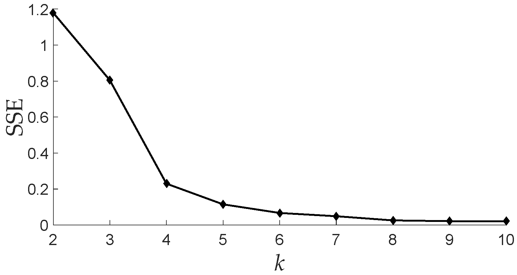
In order to make the effect of the subsequent ESCO better, this paper uses the elbow rule to determine the best k value. The elbow rule calculates the sum of intra-cluster distortion degrees, also known as the sum of squared errors (SSE) [25], and its calculation equation is shown in Equation (22).
where k is the number of clusters; represents the ith cluster; x is the sample point in ; and represents the average value of all sample data in .
Assuming that x data are clustered by k-means, when the value of k is 1, it means that all data are divided into one cluster. It can be found from Equation (22) that the SSE is the maximum. When the value of k is x, it means that each data becomes a cluster independently, so the SSE is 0. Therefore, with the increase in the k value, the SSE will gradually decrease until a critical point. After this point, the SSE will no longer decrease significantly if the k value continues to increase. If the relationship curve between the k value and SSE is drawn, it should decrease and then tend to be stable on the whole. The k value corresponding to the point in the curve where the SSE drops fastest, that is, the critical point mentioned above, is the optimal k value.
3.3. Determination of Weighting Factors of Multi-Objective Functions
For multi-objective optimization, the determination of the weighting factor of each objective is the key. Because each goal cannot be optimal at the same time, it must have its own weight, so the distribution of weight becomes the focus. According to different clustering periods, this paper adopts the fuzzy comprehensive evaluation (FCE) method to assign the weighting factor of each objective function in each period [26], and its calculation equation is as follows:
where is the overweight weighted value of the ith objective function, calculated according to Equation (24); is the number of objective functions.
where is the actual value of the ith objective function, generally taking the average value; is the maximum allowable value of the ith objective function, generally taking the maximum value.
4. Model-Solving Method
Particle swarm optimization (PSO) is used to solve the model [27]. Because the basic particle swarm is searching for continuous space, it is also called continuous particle swarm. However, the ESCO of the distribution network mentioned in this paper includes the optimization of the ES location and capacity. Among them, the position is a discrete variable, and the capacity is a continuous variable. Therefore, it is necessary to improve the basic particle swarm optimization. In this paper, hybrid particle swarm optimization (HPSO) is proposed, that is, discrete PSO is used in the location search of ES, and continuous PSO is used in the capacity search.
Assuming that there are N particles in the D-dimensional search space, and each particle represents a solution, the position of the ith particle is
The speed of the ith particle is
The optimal position searched by the ith particle is [28]
The optimal location searched by the group is
The velocity-position updating equation of basic PSO is adopted, in which the particle velocity updating equation is as follows:
where t is the number of iterations; is the velocity of the ith particle in the tth iteration; ω is the inertia weighting factor; and are the individual learning factor and global learning factor, respectively; is a random number between 0 and 1; is the position of the ith particle in the tth iteration; is the historical optimal position of the ith particle in the dth iteration, that is, the optimal solution obtained by the ith particle search after the tth iteration; is the historical optimal position of the population in the dth dimension in the tth iteration, that is, the optimal solution in the whole particle population after the t iteration.
The location update equation is as follows:
Discrete PSO is to process the position of particles by discrete points after the velocity-position update [29]. For example, in this paper, the access location of ES is the distribution network node, and for the distribution network with N independent nodes, the location of ES is an integer from 1 to N. Because each particle is a natural number in the interval of [1, N] after updating its position, it may be a decimal (let this number be g and its decimal part be {g}, so there is ( < 1)), so this paper makes the following provisions: the decimal part is rounded, that is,
The steps of the HPSO algorithm mainly include the following steps:
Step (1) Initialize the position and velocity of each particle in the population randomly;
Step (2) Evaluate the fitness of each particle, and store the position and fitness of each particle in the , and then select the individual with the best fitness and store it in ;
Step (3) Update the velocity and position of particles according to Equation (29) and Equation (30), respectively;
Step (4) For the position of each particle of the ES position optimization variable, discrete points are processed according to Equation (31);
Step (5) Compare each particle with its previous optimal position, and if it is better, take it as the current optimal position;
Step (6) Compare all the current with those of the last iteration cycle , and update ;
Step (7) If the stop condition is met (the accuracy requirement or the maximum number of iterations is reached), the iteration is terminated; otherwise, return to Step (2).
The inertia weighting factor ω can be understood as the degree of trust of particles in their current state of motion, and particles move inertia according to their own velocity. The larger ω is, the stronger the ability to explore new areas, the stronger the global optimization ability, but the weaker the local optimization ability. Therefore, a larger ω is beneficial to a global search and jumping out of local extremum. The smaller ω is beneficial to a local search and making the algorithm converge to the optimal solution quickly. Therefore, a linear change strategy of adaptive adjustment is proposed [30]: with the increase in iteration times, ω decreases continuously, and the calculation equation is as follows:
where and are the maximum and minimum values of the inertia weighting factor, respectively; Iter is the current iteration time; and is the maximum number of iterations.
5. Example Analysis
5.1. Basic Data
In this paper, an example based on IEEE33 nodes is used to verify the feasibility and effectiveness of the proposed model. See reference [27] for a system diagram and network parameters. The voltage reference value is 12.66 kV and the power reference value is 100 MVA. Select the PV and load data of the maximum load day in a certain area for analysis. See Table 1 for the access position of each unit in this system, and see Figure 1 and Figure 2 for the load and PV curves, respectively. In this example, the PV access ratio is 78.4%. See Table 2 for the electricity price data in each period, Table 3 for the parameters involved in the constraint conditions, Table 4 for the parameters involved in the cost function and Table 5 for the parameters involved in HPSO. In this paper, Matlab (version R2016a) software is used to write distributed power sources into the program of the power flow calculation part of this 33-node distribution network, so as to connect them to the distribution network. Based on the Matlab programming software, the HPSO algorithm proposed in this paper is used for ESCO of the distribution network of this example for one day to verify the effectiveness of the model proposed in this paper.

Table 1.
Grid-Connected Nodes of Units.
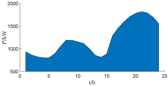
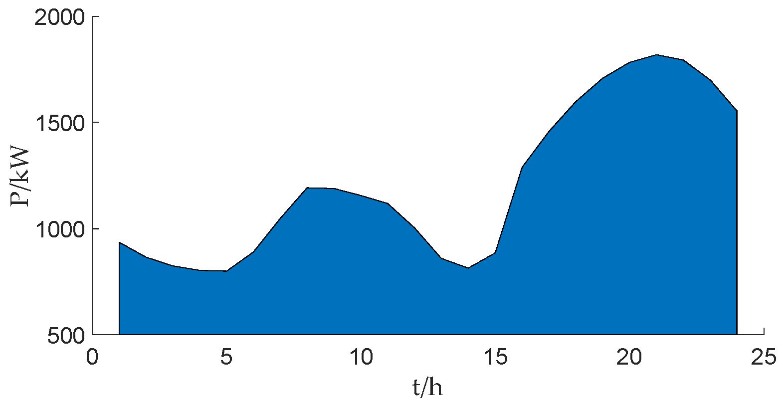
Figure 1.
Maximum load–daily load output curve.
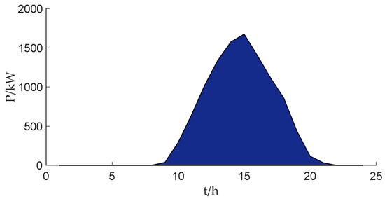
Figure 2.
Maximum load–daily photovoltaic output curve.
Table 2.
Electricity price data at each time.
Table 3.
Parameter settings in constraints.
Table 4.
Parameter settings in cost.
Table 5.
Parameter settings in HPSO.
5.2. Determine the Multi-Objective Weighting Factors
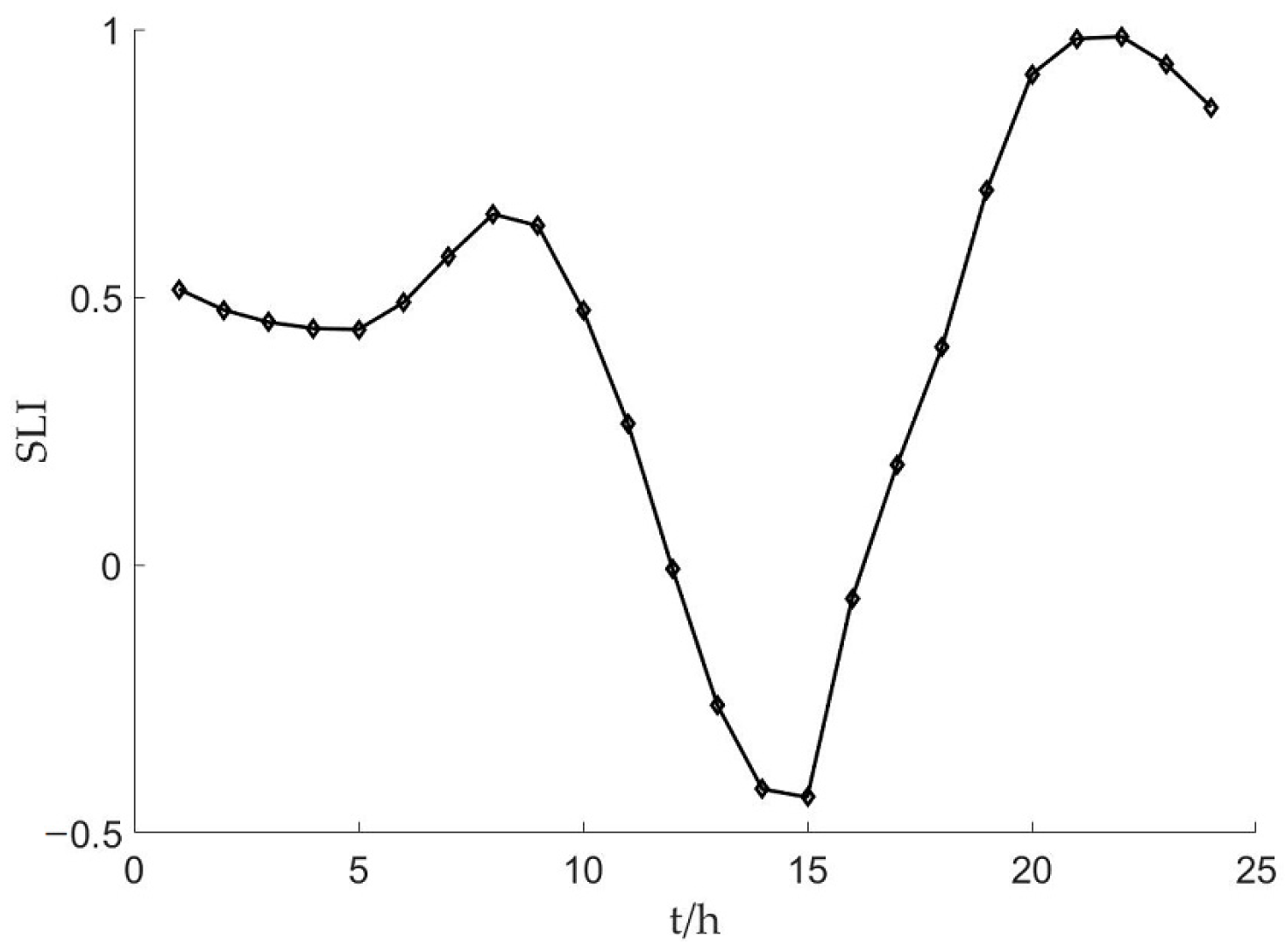
Calculate the SLI according to Equation (21) to obtain the 24 h SLI curve (see Figure 3), and then seek the optimal k value of the SLI curve by using the elbow rule, and the SSE curve is shown in Figure 4.
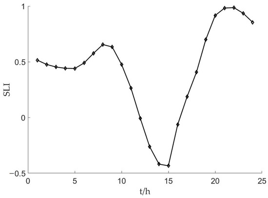
Figure 3.
SLI curve.
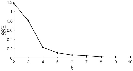
Figure 4.
SSE curve.
It can be found that after k = 4, the SSE changes slowly, and the curve tends to be stable, so the optimal k value is 4, and the whole day is grouped into 4 periods for 24 h, as shown in Table 6.
Table 6.
Period clustering results.
See Table 7 and Table 8, respectively, for the actual value data and maximum allowable value data of each objective function factor in each period.
Table 7.
Actual value data in each period.
Table 8.
Maximum allowable value data in each period.
To determine the weighting factor of each objective function in each period, see Table 9.
Table 9.
Weighting factor results of each objective function in each period.
In this paper, the following scenes are optimized for ES configuration:
Scene 1: The number of the grid-connected ES set is 2;
Scene 2: The number of the grid-connected ES set is 3;
Scene 3: The number of the grid-connected ES set is 4.
5.3. Analysis of Optimization Results Based on HPSO
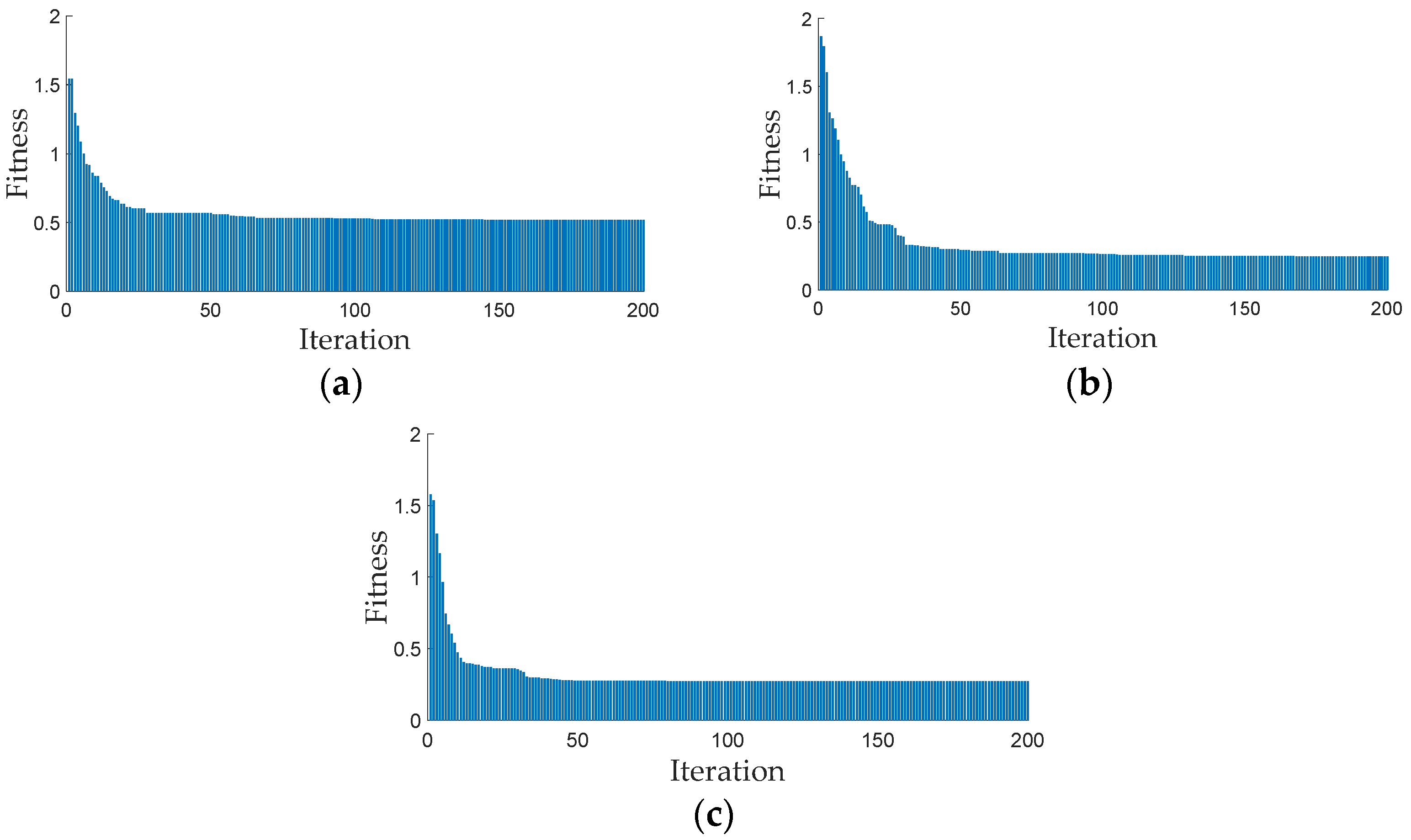
The model proposed in this paper is solved by the HPSO algorithm, and the objective function results, the optimal location of the ES grid connection and the optimal capacity (the unit of ES capacity is kW·h) in each scene are obtained, as shown in Table 10. In addition, the optimization results also include the fitness function results, voltage deviation results, GT output results and ES output results, as shown in Figure 5, Figure 6, Figure 7 and Figure 8, respectively.
Table 10.
Objective function and ES configuration results.

Figure 5.
Fitness function results: (a) scene 1; (b) scene 2; and (c) scene 3.
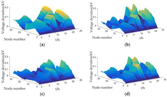
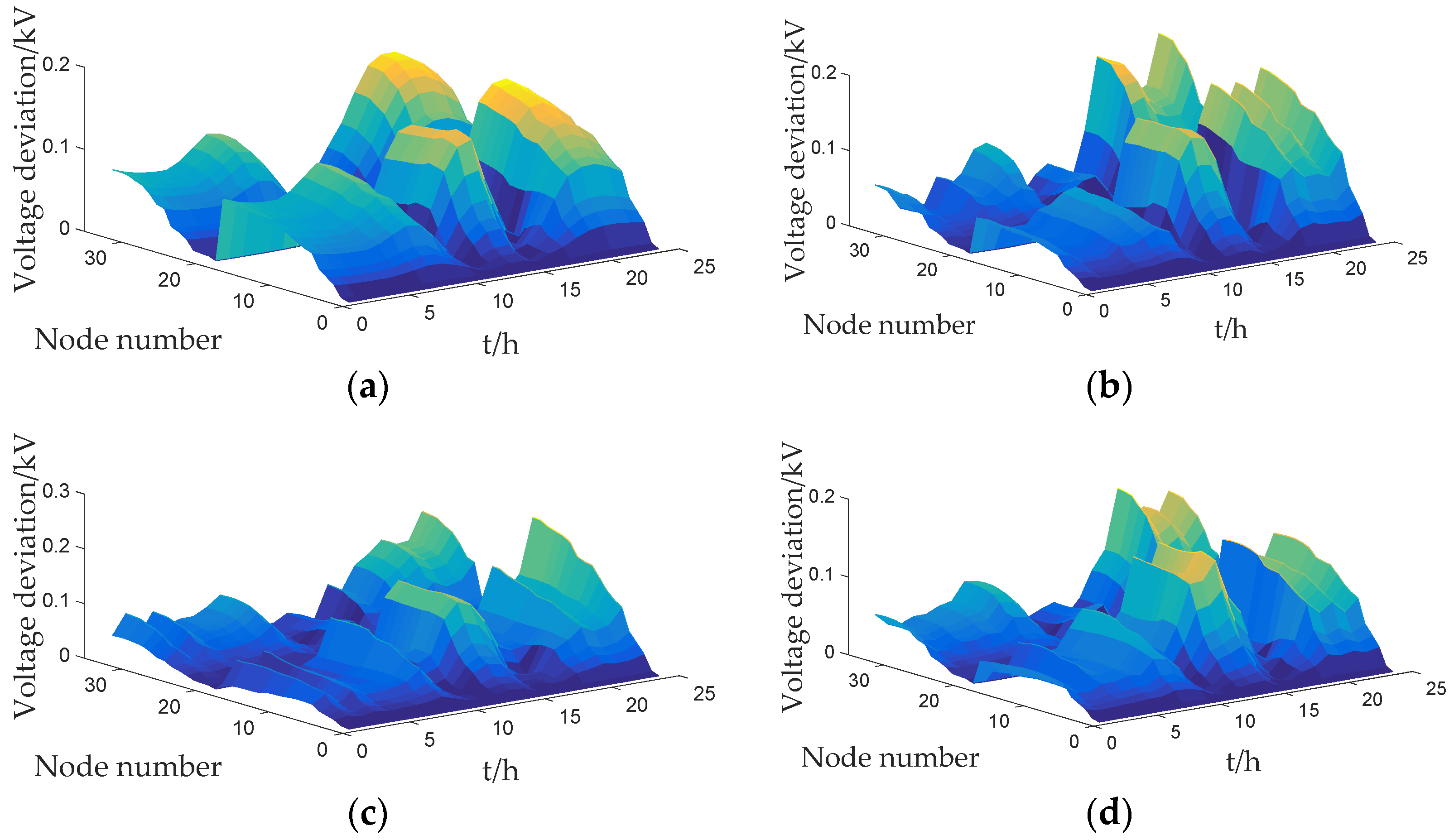
Figure 6.
Voltage deviation results: (a) before optimization; (b) scene 1; (c) scene 2; and (d) scene 3.
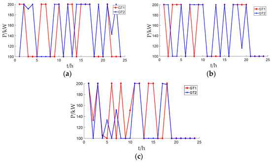
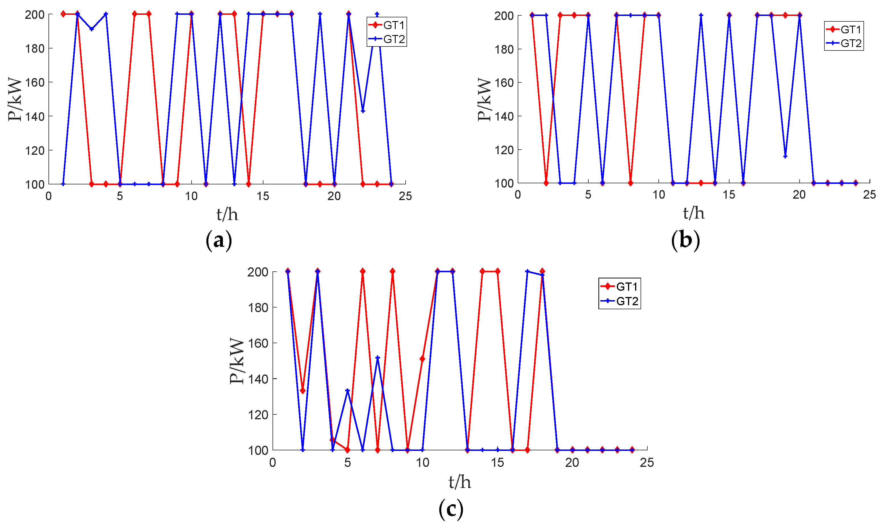
Figure 7.
GT output results: (a) scene 1; (b) scene 2; and (c) scene 3.

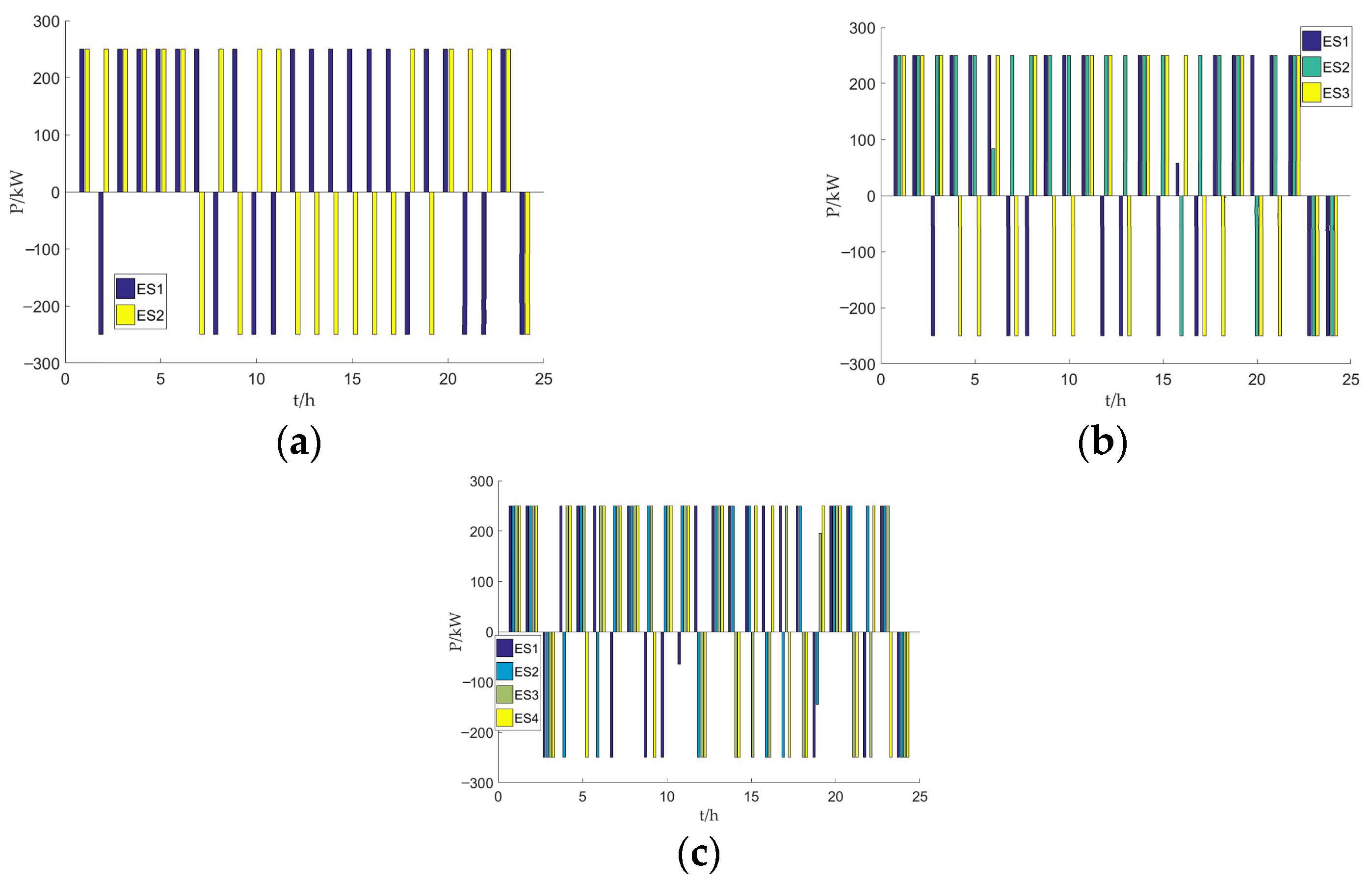
Figure 8.
ES output results: (a) scene 1; (b) scene 2; and (c) scene 3.
In the above figure, the ordinate is the fitness function value, that is, the objective function value, and the abscissa is the iteration number. Obviously, with the increase in the number of iterations, the value of the objective function is getting smaller and smaller at first, and then the degree of reduction is getting smaller and smaller until it basically does not change (when the number of iterations is about 30). The authors of this paper think that this change tends to be stable.
Among them, the specific results of the total operating cost are shown in Table 11.
Table 11.
Specific results of total operating cost.
Before optimization: and are both 0, because the GT is not connected at this time, and there is no power generation cost and environmental pollution. The three objective function values are the highest.
Scene 1: The total voltage deviation, the total power loss and the total operating cost are reduced by 10.64%, 8.75% and 19.27%, respectively, compared with those before optimization. The output of the GT and ES reaches the limit at all periods. Compared with the other two scenes, the total operating cost in this scene is the lowest, among which is the lowest, because the ES has the least access and the least output in this scene. The total voltage deviation and total power loss are the highest, which is because the number of ES accesses is small and the ability to adjust the voltage and network loss is weak.
Scene 2: The total voltage deviation, the total power loss and the total operating cost are reduced by 16.94%, 17.47% and 15.61%, respectively, compared with those before optimization. The output of the GT connected to node 4 reaches the lowest limit at most periods, while the output of the GT connected to node 25 is at the highest limit at most times.
Scene 3: The total voltage deviation, the total power loss and the total operating cost are reduced by 20.12%, 23.24% and 12.39%, respectively, compared with those before optimization. The output of the two GTs reached the limit throughout the whole day. Compared with the other two scenes, the total operating cost in this scene is the highest, and is the highest, because the ES has the most access and the most output. In addition, is the lowest, because the source–load imbalance in this scene has been greatly improved, and the GT has less output, so is also the lowest. The total voltage deviation and total power loss are the lowest, because the number of ES accesses is large, and the ability to adjust the voltage and network loss is strong.
It can be found that the fitness function in the three scenes shows a downward trend and then tends to be stable, which verifies the effectiveness of the HPSO algorithm proposed in this paper. In addition, the results of each objective function in the three scenes are effectively reduced compared with those before optimization, which verifies the effectiveness of the ESCO model established in this paper. However, with the increase in the number of ES connected to the grid, compared with the previous scene, the declining proportion of and is reduced, so the ES should be accessed as widely as possible but not too much. It can be found that 24 h a day is clustered into 4 different periods according to the SLI, and the optimization effect is the best when the number of ES installations is 4 in scene 3. Therefore, it can be considered that the optimal number of ES installations should be the number of time periods clustered according to the SLI. If there are too many ES installations, the operation and maintenance costs will be very high, which will lead to a poor economy. The method in this paper is very effective for improving the stability and economy of a distribution network, especially for a distribution network with a high proportion of photovoltaic. Using the ESCO model established in this paper, the configuration quantity, installation location and capacity of the ES can be determined under the situation of distribution network topology and load setting, thus verifying that the model proposed in this paper has good engineering practice guiding significance and practical application value.
6. Conclusions
The research on the ESCO method of a distribution network with a high proportion of PV can ensure the efficient use of ES and improve the voltage stability and power quality of a distribution network. In this paper, the ESCO model is established, and the model is solved by the HPSO algorithm. The effectiveness of this method is verified by an IEEE33-bus example. Because the model contains intermittent output energy, that is, PV, it may lead to power fluctuation and power quality degradation in the distribution network, and ESCO can effectively improve this problem. The conclusions are as follows:
- (1)
- Calculate the photovoltaic and load output data for 24 h a day, and obtain the SLI data for 24 h. These 24 data are clustered, so that one day is clustered into different periods, and the weighting factors of multi-objective functions in each period are calculated, which makes the determination of the weighting factor more in line with the actual operation of the distribution network.
- (2)
- The results of solving the model by using the HPSO algorithm proposed in this paper show that the results of each objective function in the three scenes are effectively reduced compared with those before optimization, which shows that the proposed method can solve the problems of the voltage exceeding the limit and power loss caused by an unbalanced source and load, and improve the economy of the distribution network.
- (3)
- According to the comparison of the optimization results under three scenes, it can be seen that for the distribution network with a high proportion of PV, in order to improve the operation performance of the distribution network, the ES should be connected to the distribution network as widely as possible, and the optimal number of installations should be the number of time periods clustered according to the SLI.
Author Contributions
Conceptualization, F.Z. and X.M.; methodology, X.M.; software, F.Z.; validation, F.Z., X.M. and T.X.; formal analysis, X.M.; investigation, T.X. and Y.S.; resources, T.X. and Y.S.; data curation, Y.S.; writing—original draft preparation, F.Z.; writing—review and editing, X.M.; visualization, H.W.; supervision, X.M.; project administration, H.W.; funding acquisition, H.W. All authors have read and agreed to the published version of the manuscript.
Funding
This research was funded by the Youth Program of the National Natural Science Foundation of China (grant number 61903264).
Informed Consent Statement
Informed consent was obtained from all subjects involved in the study.
Data Availability Statement
Not applicable.
Conflicts of Interest
The authors declare no conflict of interest.
References
- Singh, P.P.; Palu, I. State coordinated voltage control in an active distribution network with on-load tap changers and photovoltaic systems. Glob. Energy Interconnect. 2021, 4, 117–125. [Google Scholar] [CrossRef]
- Lei, X.; Tianjun, J.; Yi, C.; Weizhou, W. Boundary Simulation of PV Accommodation Capacity of Distribution Network and Comprehensive Selection of Accommodation Scheme. Power Syst. Technol. 2020, 44, 907–916. [Google Scholar]
- Chongwei, Y.; Xu, L.; Lan, M. Research on Voltage Control of Low Voltage System Based on High-proportion Photovoltaic Access. Electr. Drive 2022, 52, 60–67. [Google Scholar]
- Ji, L.; Junxiao, C.; Yunge, Z.; Shiping, E.; Chuihui, Z. Two-stage reactive power chance-constrained optimization method for an active distribution network considering DG uncertainties. Power Syst. Prot. Control 2021, 49, 28–35. [Google Scholar]
- Jingqi, L.; Dan, W.; Hua, F.; Dongjun, Y.; Rengcun, F.; Zixia, S. Hierarchical Optimal Control Method for Active Distribution Network with Mobile Energy Storage. Autom. Electr. Power Syst. 2022, 46, 189–198. [Google Scholar]
- Xiangjing, S.; Sili, C.; Yang, M.; Yang, F. Sequential and Optimal Placement of Distributed Battery Energy Storage Systems Within Unbalanced Distribution Networks Hosting High Renewable Penet rations. Power Syst. Technol. 2019, 43, 3698–3706. [Google Scholar]
- Zhiyu, M.; Jiangye, M.; Peiqiang, L.; Jiangyu, C. Optimal Configuration of Energy Storage in Distribution Network Based on Improved Gray Wolf Algorithm. Proc. CSU-EPSA 2022, 34, 1–8. [Google Scholar]
- Yulong, J.; Zengqiang, M.; Liqing, L.; Qukai, Y. Comprehensive optimization method of capacity configuration and ordered installation for distributed energy storage system accessing distribution network. Electr. Power Autom. Equip. 2019, 39, 1–7. [Google Scholar]
- Qunmin, Y.; Xinzhou, D.; Jiahao, M.; Yongxiang, M. Optimal configuration of energy storage in an active distribution network based on improved multi-objective particle swarm optimization. Power Syst. Prot. Control 2022, 50, 11–19. [Google Scholar]
- Xiaoyi, L.; Tianyuan, F. Energy-storage configuration for EV fast charging stations considering characteristics of charging load and wind-power fluctuation. Glob. Energy Interconnect. 2021, 4, 48–57. [Google Scholar] [CrossRef]
- Li, C.; Zhang, H.; Zhou, H.; Sun, D.; Dong, Z.; Li, J. Double-layer optimized configuration of distributed energy storage and transformer capacity in distribution network. Int. J. Electr. Power Energy Syst. 2023, 147, 108834. [Google Scholar] [CrossRef]
- Cao, J.; Wang, C.; Huo, C.; Luo, C.; Tao, D.; Wu, X. Optimal planning of electric vehicle charging stations considering the load fluctuation and voltage offset of distribution network. J. Electr. Power Sci. Technol. 2021, 36, 12–19. [Google Scholar]
- Al-Kaabi, M.; Dumbrava, V.; Eremia, M. Single and Multi-Objective Optimal Power Flow Based on Hunger Games Search with Pareto Concept Optimization. Energies 2022, 15, 8328. [Google Scholar] [CrossRef]
- Qipeng, M.; Zhenghang, H.; Yu, Z.; Shunji, Y.; Zhuo, C.; Qifei, L. Network Partition and Voltage Coordination Control of Distributed PV Power Distribution Network with High Permeability. Power Syst. Clean Energy 2023, 39, 93–102+108. [Google Scholar]
- Zhigang, M.; Zhinong, W.; Sheng, C.; Yuping, Z.; Tonghua, W. Active-Reactive Power Optimal Dispatch of AC/DC Distribution Network Based on Soft Open Point. Autom. Electr. Power Syst. 2023, 47, 48–58. [Google Scholar]
- Qianyun, S. A bi-level optimization planning method for a distribution network considering different types of distributed generation. Power Syst. Prot. Control 2020, 48, 53–61. [Google Scholar]
- Xiaotao, Z.; Yichao, W.; Wenxian, Z.; Qixian, W.; Aijun, W. System Performance and Pollutant Emissions of Micro Gas Turbine Combined Cycle in Variable Fuel Type Cases. Energies 2022, 15, 23. [Google Scholar] [CrossRef]
- Mingjie, Y.; Yangyu, H.; Haixia, Q.; Fang, L.; Xingkai, W.; Xiaoyang, T.; Jie, Z. Optimization of day-ahead and intra-day multi-time scale scheduling for integrated power-gas energy system considering carbon emission. Power Syst. Prot. Control 2023, 51, 96–106. [Google Scholar]
- Shuqiang, Z.; Lei, H.; Zhiwei, L.; Yuhang, Y.; Shuting, M. Day-ahead optimal Scheduling of Active Distribution Network by Related Opportunity Goal Planing. J. North China Electr. Power Univ. 2021, 48, 1–10. [Google Scholar]
- Shu, Z.; Jingtao, Z.; Mingxiang, L. Scheduling Method of Wind Power PhotoVoltaic Photothermal Complementary Generator Set Based on K·means Clustering Algorithm. Electr. Mach. Control. Appl. 2023, 50, 61–66. [Google Scholar]
- Min, Z.; Jianxue, W.; Xiuli, W.; Xiaoyu, C.; Yang, C. Bilateral trading mechanism and model of peak regulation auxiliary service market for renewable energy accommodation. Electr. Power Autom. Equip. 2021, 41, 84–91. [Google Scholar]
- Pawitan, G.A.H.; Kim, J.-S. MPC-Based Power Management of Renewable Generation Using Multi-ESS Guaranteeing SoC Constraints and Balancing. IEEE Access 2020, 8, 8. [Google Scholar] [CrossRef]
- Hongtao, S.; Fanding, Y.; Lun, S.; Linqing, L.; Mengyu, L.; Zihe, D.; Huan, Y. Comprehensive Optimal Planning of Multi-obj ective Distribution Network Reconfiguration and DG Regulation Considering DG and Load Sequence. Mod. Electr. Power 2022, 39, 182–192. [Google Scholar]
- Fangfang, Z.; Xiaofang, M.; Lidi, W.; Nannan, Z. Operation Optimization Method of Distribution Network with Wind Turbine and Photovoltaic Considering Clustering and Energy Storage. Sustainability 2023, 15, 2184. [Google Scholar] [CrossRef]
- Fangfang, Z.; Xiaofang, M.; Lidi, W.; Nannan, Z. Power Flow Optimization Strategy of Distribution Network with Source and Load Storage Considering Period Clustering. Sustainability 2023, 15, 4515. [Google Scholar] [CrossRef]
- Xiaofang, M.; Lidi, M.; Xiaoning, W.; Yingnan, W.; Ran, L. Improve operation characteristics in three-phase four-wire low-voltage distribution network using distributed generation. Power Syst. Technol. 2018, 4091–4100. [Google Scholar]
- Mengyi, L.; Xiaoyan, Q.; Zhirong, Z.; Changshu, Z.; Youlin, Z. Multi-objective reactive power optimization of distribution network considering output correlation between wind turbines and photovoltaic units. Power Syst. Technol. 2020, 44, 1892–1899. [Google Scholar]
- Djidimbélé, R.; Ngoussandou, B.-P.; Kidmo, D.K.; Kitmo; Bajaj, M.; Raidandi, D. Optimal sizing of hybrid Systems for Power loss Reduction and Voltage improvement using PSO algorithm: Case study of Guissia Rural Grid. Energy Rep. 2022, 8, 86–95. [Google Scholar] [CrossRef]
- Qing, L.; Hongli, Z.; Longxiong, M.; Ningxin, Z. Optimization of Geomagnetically Induced Current Suppression Based on Multi-Objective Discrete Particle Swarm Optimization Algorithm and Effect Evaluation. J. Xi’an Jiaotong Univ. 2021, 55, 90–98. [Google Scholar]
- Sellami, R.; Sher, F.; Neji, R. An improved MOPSO algorithm for optimal sizing & placement of distributed generation: A case study of the Tunisian offshore distribution network (ASHTART). Energy Rep. 2022, 8, 6060–6975. [Google Scholar]

Disclaimer/Publisher’s Note: The statements, opinions and data contained in all publications are solely those of the individual author(s) and contributor(s) and not of MDPI and/or the editor(s). MDPI and/or the editor(s) disclaim responsibility for any injury to people or property resulting from any ideas, methods, instructions or products referred to in the content. |
© 2023 by the authors. Licensee MDPI, Basel, Switzerland. This article is an open access article distributed under the terms and conditions of the Creative Commons Attribution (CC BY) license (https://creativecommons.org/licenses/by/4.0/).