Abstract
The effects of environmental pollution and Industry 4.0 on a sustainable environment are the main topic of this study, which may be regarded as a complement to the literature on energy and the environment. The paper aims to investigate the relation between Industry 4.0 (I4.0) and environmental sustainability, which is very important for policymakers, practitioners, and company executives in the period of Industry 4.0 in Turkey. To this end, natural gas consumption and technology patents as control variables of Industry 4.0, in addition to the variables of environmental pollution and economic growth, were selected during the period of 1988 to 2022 using Markov switching VAR (MS-VAR), Markov switching Granger causality (MS-GC), Fourier VAR (FVAR), and Granger causality (FGC) techniques. The reason for covering the period starting in 1988 is its recognition as the beginning of the Industry 4.0 era with AutoIDLab in 1988. According to the causality results, there was unidirectional causality running from technology patents to environmental pollution in the results of both MS-GC and FGC. However, the directions of causality between natural gas consumption and environmental pollution, and between economic growth and environmental pollution differed between regimes in the MS-GC model. Bidirectional causality was determined between economic growth and environmental pollution in the first MS-GC regime. However, in the second regime, unidirectional causality from economic growth to environmental pollution was determined. The causality direction determined by Fourier causality gave the same result with the second regime. A similar finding was observed in the direction of causality between natural gas consumption and CO2 emissions. While MS-GC determined unidirectional causality from natural gas consumption to environmental pollution in the first regime, a bidirectional causality result between GC and environmental pollution was determined in the second regime. The FGC result was similar to the second regime result. And lastly, the MS-GC and FGC methods determined unidirectional causality from Industry 4.0 to environmental pollution.
1. Introduction
Industry 4.0 is critical in improving the production processes of various industries, including the oil and gas industry. Thanks to the adoption of Industry 4.0 technology, which has resulted in the optimization and enhanced performance of the manufacturing industry, there has been a significant movement from traditional manufacturing enterprises to smart factories [1,2]. Industry 4.0 refers to modern technology, including cyber-physical systems, the Internet of things (IoT), big data, the cloud, automation, cybersecurity, and artificial intelligence. Furthermore, IoT, cloud, big data, and analytics were designated as the four foundation technologies of Industry 4.0 in [3,4,5]. Big data and analytics are essential enablers for advanced applications of Industry 4.0, while cloud services offer simple access to information and services, and IoT addresses communication problems. To this end, advanced technologies have addressed some of the industry’s top concerns, including supply chain resilience, exploration, analysis, safety, and sustainability. In real terms, the oil and gas supply chain has already undergone positive adjustments.
While some sectors are transforming under the influence of Industry 4.0, the need for energy consumption is increasing. Under the influence of Industry 4.0, there has been a gradual increase in natural gas consumption, especially since the beginning of 2000. The main reasons for the increase in natural gas consumption are that it is an essential source of electricity production and the most crucial energy input of the industrial sector, with an increase in individual consumption. In this process, analysis methods that use large data groups have just started to be used in production to increase the quality of production and impact energy consumption. Energy consumption is one of the leading causes of environmental pollution, a critical problem for our world. Compared to the average temperature between 1850 and 1900, global surface temperatures increased by 1.09 °C over the past 10 years (2011–2020) [6]. Around the world, there was a rise of 1.59 °C. Global temperatures are expected to rise by 1.5 °C or more in the next 20 years due to GHG emissions, which have caused an average warming of ~1.1 °C since the 1850–1900 period. The hazardous limit of 2 °C must not be surpassed to safeguard populations and ecosystems from the overwhelming effects of climate change. Hence, restricting global temperature increases to 1.5 °C is crucial for the same reason [6].
In the era of Industry 4.0, governments are concerned about reducing energy use, lessening CO2 emissions, and saving money to improve energy efficiency and limiting disruptions caused by I4.0 technologies. These issues also deal with how to evaluate and select the appropriate energy technology in accordance with sustainability principles [7]. The International Energy Agency (IEA) estimates that the widespread use of current digital technology may reduce production costs in the oil and gas industry by 10% to 20%. In this respect, businesses are spending more on applications that may benefit from digital technology, such as inventory management and logistics. Among the applications taking off in the oil and gas industry are digital process optimization and predictive maintenance for equipment.
The influence of the Fourth Industrial Revolution on energy is mainly unknown (for example, lack of access to energy), while it presents several chances for sustainability (addressing social, economic, and environmental concerns) [8]. Hence, Industry 4.0 has created a situation where businesses must make wise judgments to maintain an advantage over the competition [9]. The same can be true for the environment and energy consumption. Environmental pollution is a major problem and, in the era of Industry 4.0, their bidirectional impact should be assessed. Some studies have analyzed the relationship between energy consumption and Industry 4.0, whereas, in this study, we focus on natural gas consumption and its relationship with the environment, enabling the dimensions of environmental pollution, as well as policies to reduce it, to be intensively discussed.
A mentioned above, some papers discussed the relationship between the energy sector and Industry 4.0. In line with the Industry 4.0 era, Lu et al. [10] evaluated the leading technologies and application scenarios of the oil and gas (O&G) industry, assessed the benefits and challenges of implementation, and offered strategies and policies to support the sector’s adoption of Industry 4.0. The authors of [11,12,13] also presented vital studies for the O&G industry. Onyeme and Liyanage [14] investigated the Industry 4.0 (I4.0) maturity models (MMs) that are currently accessible for manufacturing sectors and investigated how well they were implemented in the oil and gas (O&G) upstream sector. The authors of [15] highlighted IoT implementation conflicts among countries, while adaptation issues for I4.0 technologies, such as cloud computing and robotics implementations, were highlighted by [16]. Raj et al. [17] explored the obstacles to adopting I4.0 technology. Among these impediments, Breunig et al. [18] cited the high R&D expenses of I4.0. Jasiulewicz-Kaczmarek et al. [19] analyzed Industry 4.0 technologies for sustainable asset lifecycle management. Recently, Chauhan et al. [20] demonstrated digitalization’s inherent and extrinsic constraints in the context of I4.0. In addition to the problems listed above, the effects of I4.0 on the sustainability of production and the environment are being questioned. According to Lin et al. [21], the technologies launched under the notion of I4.0 necessitate an innovation strategy followed by businesses and governments focusing on environmental issues. Blockchain technology is one of the technologies created as part of the I4.0 development. Nonetheless, cryptocurrency technology is regarded as the most significant technological innovation in the context of financial technologies within I4.0 [22]. However, the environmental effects of blockchain technologies, in addition to other I4.0 technologies, are expected to put pressure on the environment.
Kluczek et al. [23] examined how Industry 4.0 places demands on business owners to make energy-efficient decisions in order to compete in the market. This study introduced prospect theory (PT) for decision making in Industry 4.0 to choose the best energy technology. Bildirici and Ersin [2] employed internet and communications technology (ICT) exports, research and development (R&D), artificial intelligence (AI), ICT technology patents, and Bitcoin as proxies for Industry 4.0. However, these variables could only be obtained after 2000. The period of 2000–2021 can be considered short when using annual data. For this reason, we use technology patents as a proxy variable for Industry 4.0. On the other hand, various studies [24,25] have highlighted the inclined energy consumption due to I4.0 technologies, in addition to Bitcoin mining activities which significantly burden the environment.
On the other hand, some papers analyzed the relationship linking natural gas consumption, economic growth, and environmental pollution. The initial literature collection was a time series data investigation [26,27,28,29]. The second, more condensed body of literature used panel data model analysis as its foundation [29,30,31,32,33,34,35,36,37]. Later, Zamani [38] used the vector error correction model (VECM), Hu et al. [39] applied cointegration and causality for the United States (US), and the authors of [40] investigated Taiwan. They found a long-term relation between natural gas consumption (NGC) and economic development. Furthermore, some papers found a unidirectional causality between NGC and economic growth in multiple nations, including [41,42] for the US, [43] for the Soviet Union, [44] for Nigeria, [45] for Iran, [46] for the United Kingdom (UK), US, and Poland, [32] for New Zealand and Australia, [31] for Pakistan, Bangladesh, Nepal, India, and Sri Lanka, and [47] for Pakistan. Considering the studies conducted after 2020, according to [48], Nigeria’s economic growth was boosted by using natural gas. Additionally, the authors used nonlinear estimate methods to support this assertion and concluded that the relationship between natural gas consumption and economic development is nonlinear. Awodumi and Adewuyi [49] discovered that increasing Gabon’s natural gas use effectively boosted economic growth and reduced environmental pollution. However, they asserted that natural gas usage in Nigeria had effects that slowed growth. According to Etokakpan [50], economic growth and natural gas consumption are both impacted by one another; as a result, a feedback connection was established. In the context of the top CO2-emitting global economies, Azam et al. [51] could not show any causality relationship between natural gas use and economic development.
However, these papers did not analyze cointegration and causality among Industry 4.0, natural gas consumption, economic growth, and environmental pollution for Turkey. This paper aimed to analyze the causality among economic growth, natural gas consumption, and environmental pollution, and Industry 4.0 using Markov switching VAR (MS-VAR), MS-Granger causality (MS-GC), Fourier VAR (FVAR), and Fourier Granger causality (FGC) techniques from 1988 to 2022 in Turkey. The reason for covering the period starting with 1988 is its recognition as the beginning of the Industry 4.0 era with AutoIDLab in 1988. The MS-VAR method can provide us with information about the stages of fluctuations because when economic growth is used as variable, fluctuations should be taken into account. The stage of the business cycle must be considered when analyzing the evidence of the GDP variable; otherwise, estimated parameters could be inaccurate. Some articles used the Markov switching (MS) approach to solve this issue in the context of GDP and oil price variables. The first paper that used the MS approach to evaluate oil price volatility was [52]. Later, MS-AR and MS-VAR models were used by [53,54,55,56,57,58] to examine the effects of energy prices on macroeconomic variables and/or to establish the relationship between energy consumption and economic growth. However, since the period was short, we also used the Fourier VAR and F-GC methods. On the other hand, the Fourier approach allows investigating nonlinear series or series with structural breaks with unknown forms and break dates. The simultaneous use of these methods is expected to provide an opportunity to make effective policy recommendations.
Our expectation is that, if the results in the MS-GC method differ between regimes, the results in the FGC method should be similar to those in one of the regimes. In this case, the policy recommendation will be based on the regime stages and the general interpretation. If the results are completely different, no policy recommendation will be made.
2. Methodology
2.1. Markov Switching VAR and Causality
As an alternative to a stationary linear autoregressive model, Hamilton (1989) provided a simple nonlinear framework for modeling economic time series with a permanent and cyclical component.
The MSI(.)-VAR(.) model is as follows:
Ai (.) shows the coefficients of the lagged values of the variable in different regimes, and shows the variance of the residuals in each regime. defines the dependence of the mean of the K-dimensional time series vector on the regime variable st.
In an MS-VAR model, st is governed by a Markov chain, and
where p includes the probability parameters. That is, the state in period t would depend only on the state in period t − 1. On the other hand, the conditional probability distribution of yt is independent of st − 1, i.e., .
It is assumed that s follows an irreducible ergodic M state Markov process with the transition matrix, defined as
The Markov chain is ergodic and irreducible; a two-state Markov chain with transition probabilities pij with unconditional distribution is presented in the above equations. There are different methods to estimate the MS models, such as the maximum likelihood estimate (MLE) and the expectation maximization (EM) suggested by Hamilton.
The EM algorithm was created to estimate the parameters of a model where the observed time series depends on an unobserved or hidden stochastic variable. To make an inference, an iterative method was used for t = 1, 2, …, T, while taking the previous value of this probability,
This inference can be demonstrated as
where i = 1, 2, denotes the information set, and is the vector of parameters to be estimated.
The iterative estimation technique can be used to make an inference as
The conditional log likelihood can be given as
The authors [56,57] used the MS-VAR and MS causality models in their research, and they used two different models to examine the relationship between economic growth and energy consumption. These models were MSIA(.)-VAR(.) and MSIAH(.)-VAR(.) MSIA(.)-VAR(.) is given as
where , and Ai (.) represents the coefficients of the lagged values of the variables in the different regimes. According to these models, where describes the variance of the residuals of each regime, symbolizes the dependence of the mean on the k-dimensional time series vector. In addition, can be defined as the regime variable. In the context of the study, the input variables are used.
We can define these input variables in matrix form as
where p is the optimum lag length and varies according to the information criterion. Additionally, the regimes here have varying characteristics. That is, the regime varies according to its previous value and probabilities [59], and it can be defined as
where represents the probability of transition from regime i to regime j. It can also be shown as
where shows k different possible regimes. The transition between regimes is determined by the Markov model. This model can be defined as
It can be shown in matrix form as follows:
The Markov chain is ergodic can irreducible, and the ergodic probability vector can be expressed as the unconditional probability of each regime. When the Markov chains are accepted as ergodic, unconditional probabilities can be used as initial values [60]. They are given by
Optimal prediction probabilities are found using
where , and symbolizes the vector of conditional densities, while 1 symbolizes a unit column vector. The estimation is made using the following equation:
2.2. Markov Switching VAR Nonlinear Granger Causality
The authors of [56,57] used the MS-Granger causality for MSIA(.)-VAR(.) and/or MSIAH(.)-VAR(.) models. The approach is described as follows:
In the dlxt vector, dlyt is Granger cause of dlxt in each j-th regime if the parameter set or sets of and are statistically different from zero.
2.3. Fourier VAR and Granger Causality
The Fourier model is defined as follows according to [1,2]:
where is i.i.d., and . For the Granger causality method, in the bivariate setting, the short-run Granger noncausalities are tested under the null hypotheses of in the first vector and in the second vector against the alternatives of and , respectively, in Equations (18) and (19) for all i. The Granger causality testing requires estimating the vector model with m optimum lag selected with an information criterion. Common criteria include Schwarz and Akaike.
3. Data
The cointegration and causality between natural gas consumption, Industry 4.0, environmental pollution, and economic growth (y) were explored using monthly data from 1988 to 2021. Every variable was changed to X = log (Xt). Data and their descriptive statistics are given in Table 1.

Table 1.
(a) Data definitions. (b) Descriptive statistics.
In Table 1b, it was presented the results of Skewness, Kurtosis and Jarque–Bera Statistics.
4. Empirical Results
The stages in this paper are given as follows: (1) the stationarity of the variables was explored using the ADF and PP tests; (2) the Johansen cointegration test was used. Since the null hypothesis of no cointegration was not rejected, innovations of the variables were evaluated using the MSVAR and FVAR methods. The results of MSVAR and FVAR methods were used to determine the direction of causality; (3) the VAR model was evaluated against an MS-VAR structure with two regimes and then with two regimes versus three to determine the number of regimes. After the regimes of the MSVAR model were determined, MS-VAR and FVAR methods were applied; (4) the causality results found by the MSVAR method were compared with those found by the Fourier VAR (FVAR) method.
In Table 2, the ADF test stated that all variables were found as I (1).
Table 2.
ADF test results.
The results of the Johansen cointegration test are shown in Table 3. We can conclude from Table 3’s findings that the null hypothesis of no cointegration was not rejected. The variables are I(1), but they are not cointegrated. In this case, for MS-Granger causality and Fourier causality, the innovations of variables dlgct, dltpt, dlcot, and dlyt were used.
Table 3.
Johansen cointegration test results.
4.1. MS-VAR and Fourier VAR Results
The MSIA(2)-VAR(1) model was established. An MS model with two different regimes where both intercept and autoregressive coefficients are regime dependent. The regimes were determined as a crisis regime or growth regime. Regime 1 consists the recessions in the early 1990s, and the recession in 2000–2001, and 2008 great recession.
The MSIA(2)-VAR(1) model suggests, according to our results, that the total lengths of the growth regimes were higher than the other regimes. In Table 4, the estimates of all the parameters of the MSIA(2)-VAR(1) model using EM algorithm are reported. This model is tested for linearity using the LR linearity statistics assuming the null and alternative hypotheses to be a linear model and a MS model, respectively. All the statistics support the existence of non-linearity. The transition probability matrix was ergodic. Additionally, this matrix could not be irreducible. The regime probabilities were found as Pr(st=1| st – 1 = 1) = 0.72, Pr(st = 2|st – 1 = 2) = 0.91. The findings suggest that the persistence of the second regime was higher than that of the first.
Table 4.
MSIA(2)-VAR(1) results.
The dependent variable in the first equation is the innovation of GC, i.e., dlgc. The dependent variable in the third equation is the innovation of CO, i.e., dlco. The estimated coefficients of GC innovations (dlgc) are significant only in the first and second regime. The sign of the coefficient of lgc(−1) on environmental pollution was positive, and the sign of the coefficient of lgc(−2) was negative. In the second regime, similar to the first regime, the sign of the coefficient of lgc(−2) was negative. Hence, natural gas consumption for lgc(−2) in both regimes can cause a decrease in carbon emissions.
As emphasized above, we solved the Fourier VAR model due to the short period. Moreover, we wanted to compare the results. We calculated two Fourier coefficients in the Fourier model.
The results are exhibited in Table 5.
Table 5.
Fourier VAR Model.
4.2. Markov Switching Causality and Fourier Causality Results
Since accurately presenting the causality findings is essential for both policy ideas and future research, this section aimed to compare the causality results on the basis of two distinct approaches. The results were similar.
The results are shown in Figure 1.
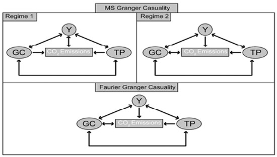
Figure 1.
Causality results.
5. Discussion
In this paper, the importance of natural gas consumption in the Industry 4.0 process and the impact of Industry 4.0 on environmental pollution in the Industry 4.0 period were evaluated using the MS-VAR, MS-GC and FVAR, FGC methods. Unlike the studies in the literature, these methods gave us information both about the direction of causality and about the signs of the coefficients of the variables. The results showed that the selected methods are important to analyze natural gas, which plays an important role in reducing environmental pollution in Industry 4.0 processes. The importance of the MS-VAR method for policy recommendations revealed by our results is similar to the results obtained in the studies conducted by [17,18,20] and the importance of the FVAR and FGC methods is similar to the results obtained by [2].
Both MS-VAR and FVAR methods showed that the sign of coefficient of natural gas on environmental pollution was negative at lag(−2). This result was found for the two regimes of the MS-VAR method and the FVAR method. In the same way, the Industry 4.0 variable, symbolized by the variable dltp, may also have a mitigating effect on environmental pollution. However, this situation was only valid for lag(−2) in the FVAR method and in the second regime of the MSVAR model. In the first regime and for lag(−1) in regime 2, and lag(−1) in the FVAR the sign was positive.
When the effect of economic growth on environmental pollution was analyzed, the MS-VAR model showed a coefficient with a negative sign in lag(−1) in reg1 in lag(−1) and lag(−2) in reg2, but a coefficient with a positive sign in lag(−2) in reg1 and lag(−1) in the FVAR. The coefficients and signs between economic growth and the environment were similar to those found by many studies in the literature. In the natural gas equation, when the coefficients and signs between Industry 4.0 and natural gas consumption were analyzed, the coefficient of the sign for lag(−1) in the FVAR model was positive while lag(−2) was statistically insignificant. In the MSVAR model, the signs of the coefficients were positive in both regime 1 and regime 2. Industry 4.0 increases natural gas consumption. When the effect of natural gas on carbon dioxide was analyzed, the negative sign of the coefficient for lag(2) in all models revealed the importance of natural gas consumption in the Industry 4.0 period.
The causality results have important implications in terms of policy recommendations. We compare the findings of the two models in Table 6. Since the results were generally the same in both models, we could easily use the causality results for policy recommendation.
Table 6.
Comparison of the ausality results.
When the causality results in the context of natural gas consumption and environmental pollution were compared, the causality direction for the results in the first regime of the MS-GC model was different from that in the second regime and Fourier causality (FGC). In the second regime of the MS-GC model and in FGC model, a bidirectional causality result was determined, whereas unidirectional causality from GC to environmental pollution was found for the first regime in the MS-GC model. In the MS-GC model, unidirectional causality from Industry 4.0 to environmental pollution was found in both regimes and the FGC model. Industry 4.0 was the Granger cause of environmental pollution. In the context of the coefficient signs of the variables, the negative sign of the variables at lag(−2) in regime 2 and in FVAR model showed the positive impact of tp on environmental pollution. Industry 4.0 was also a variable with positive effects on economic growth at lag(−1) in all models. The evidence of bi-directional causality among the variables was found between the variables in both regimes in the MS-GC model and FGC model. Industry 4.0 was an important variable in both environmental pollution and economic growth.
Similar results were highlighted in [1,2], who found that technology 4.0 had significant impacts on the environment. On the other hand, in the context of the relationship between natural gas and economic growth, similar results have been highlighted in the literature. Indeed, the authors of [49] discovered that increasing Gabon’s natural gas use effectively boosted economic growth and reduced environmental pollution. The authors [33,36,37,50] determined the evidence of causality between economic growth and natural gas consumption.
Natural gas can have positive effects on economic growth, as well as positive effects on the environment. Similar to our results, some papers determined the positive effects of natural gas consumption on environmental pollution. Kuang and Lin [61] found an emission reduction effect of natural gas consumption on environmental pollution. Natural gas is a vital fossil energy in the fight against air pollution as it is the least harmful fossil fuel to the environment. Our results differed slightly from the literature. Sign of coefficient of carbon dioxide emissions in lag(−1) was determined to be positive and negative for lag(−2). So, for the results in lag(−2), our results support the above judgment. Natural gas can have positive effects on economic growth, as well as positive and negative effects on the environment. Since natural gas is the most critical energy input of the industrial sector, it is an important energy source that meets the heating needs.
Moreover, bidirectional causality between Industry 4.0 and natural gas was found in both models and in both regimes in the MS-GC model. As a result of the interaction between energy technology and the adoption of I4.0, it is possible to improve the organization and quality of manufacturing processes to support the transition from a traditional production facility to one that uses extensive IT while still achieving both high manufacturing efficiency and sustainability (recovering energy, a precise measurement of energy use, etc.). At this point, ensuring supply security is of great importance.
The findings make it abundantly evident to governments and policymakers that the I4.0 shift has significantly supported environmental sustainability. As a result, governments need to increase their efforts to reduce the harmful impacts of economic output, energy use, and I4.0.
6. Conclusions
For Turkiye, the cointegration and causality of natural gas consumption, industry 4.0 environmental pollution, and economic growth during the 1988–2022 were evaluated using MS-VAR, FVAR, MS-GC, and FGC methods. First, unit root tests were applied to the data. Variables were stationary at first difference values. Among the variables, cointegration was investigated using the Johansen test. Following our result of no cointegration, the innovation of the variables was used in the MS-VAR and Fourier VAR analysis. The results we obtained under these conditions were interpreted as the result of causality. Accordingly, our results determined bidirectional causality between GC and CO in the second regime of the MS-GC model and FGC model, as well as unidirectional causality from GC to CO in the first regime of MS-GC model. There was evidence of unidirectional causality from TP to CO in both regimes and the FGC model. Industry 4.0 was the Granger cause of environmental pollution.
The increased energy demand from I4.0 has put additional strain on the environment because I4.0-related technologies require intense energy use. This is especially true for nations that generate more power from nonrenewable and fossil-fuel sources. In this regard, governments are advised to switch to renewable energy sources in order for their nations to invest in I4.0-related technology. On the other hand, renewable energy cannot be a short-term policy idea since it pollutes the environment while being produced. Consequently, as part of Industry 4.0’s exploration of synergies linking economic, social, environmental, and technological objectives, this technique offers a strategy that can be implemented into an energy-sustainable policy.
Author Contributions
Conceptualization, M.E.B. and S.B.; methodology, M.E.B., S.B. and S.Y.G.; software, M.E.B.; validation, M.E.B.; formal analysis, M.E.B.; investigation, M.E.B., S.Y.G. and S.B.; resources, M.E.B., S.B. and S.Y.G.; data curation, M.E.B., S.Y.G. and S.B.; writing—original draft preparation, M.E.B.; writing—review and editing, M.E.B. and S.Y.G.; visualization, M.E.B. and S.Y.G.; supervision, M.E.B. and S.Y.G.; project administration, M.E.B., S.Y.G. and S.B.; funding acquisition, M.E.B. All authors have read and agreed to the published version of the manuscript.
Funding
This research received no external funding.
Institutional Review Board Statement
Not applicable.
Informed Consent Statement
Not applicable.
Data Availability Statement
The data used were obtained from reliable institutions and organizations.
Conflicts of Interest
The authors declare no conflict of interest.
References
- Bildirici, M.E.; Castanho, R.A.; Kayıkçı, F.; Genç, S.Y. ICT, energy intensity, and CO2 emission nexus. Energies 2022, 15, 4567. [Google Scholar] [CrossRef]
- Bildirici, M.; Ersin, Ö.Ö. Nexus between Industry 4.0 and environmental sustainability: A Fourier panel bootstrap cointegration and causality analysis. J. Clean. Prod. 2023, 386, 135786. [Google Scholar] [CrossRef]
- Frank, A.G.; Dalenogare, L.S.; Ayala, N.F. Industry 4.0 technologies: Implementation patterns in manufacturing companies. Int. J. Prod. Econ. 2019, 210, 15–26. [Google Scholar] [CrossRef]
- Caiado, R.G.G.; Scavarda, L.F.; Gavião, L.O.; Ivson, P.; de Mattos Nascimento, D.L.; Garza-Reyes, J.A. A fuzzy rule-based industry 4.0 maturity model for operations and supply chain management. Int. J. Prod. Econ. 2021, 231, 107883. [Google Scholar] [CrossRef]
- Onyeme, C.; Liyanage, K. A Critical Review of Smart Manufacturing & Industry 4.0 Maturity Models: Applicability in the O&G Upstream Industry. In Advances in Manufacturing Technology XXXIV; University of Derby: Derby, UK, 2021. [Google Scholar]
- IPCC. Climate Change 2021: The Physical Science Basis. 2021. Available online: https://report.ipcc.ch/ar6/wg1/IPCC_AR6_WGI_FullReport.pdf (accessed on 10 October 2022).
- Grunwald, A.; Rösch, C. Sustainability assessment of energy technologies: Towards an integrative framework. Energy Sustain. Soc. 2011, 1, 3. [Google Scholar] [CrossRef]
- Nagasawa, T.; Pillay, C.; Beier, G.; Fritzsche, K.; Pougel, F.; Takama, T.; Bobashev, I. Accelerating Clean Energy through İndustry 4.0 Manufacturing the Next Revolution; A Report of the United Nations Industrial Development Organization; United Nations Industrial Development Organization: Vienna, Austria, 2017. [Google Scholar]
- Lu, J.; Jain, L.C.; Zhang, G. Handbook on Decision Making: Vol 2—Risk Management in Decision Making; Springer Science & Business Media: Berlin/Heidelberg, Germany, 2012; Volume 33. [Google Scholar]
- Lu, H.; Guo, L.; Azimi, M.; Huang, K. Oil and Gas 4.0 era: A systematic review and outlook. Comput. Ind. 2019, 111, 68–90. [Google Scholar] [CrossRef]
- Mohammadpoor, M.; Torabi, F. Big Data analytics in oil and gas industry: An emerging trend. Petroleum 2020, 6, 321–328. [Google Scholar] [CrossRef]
- Huang, B.; Tan, L.; Liu, X.; Li, J.; Wu, S. A facile fabrication of novel stuff with antibacterial property and osteogenic promotion utilizing red phosphorus and near-infrared light. Bioact. Mater. 2019, 4, 17–21. [Google Scholar] [CrossRef]
- Chen, H.; Stavinoha, S.; Walker, M.; Zhang, B.; Fuhlbrigge, T. Opportunities and challenges of robotics and automation in offshore oil & gas industry. Intell. Control Autom. 2014, 5, 48466. [Google Scholar]
- Onyeme, C.; Liyanage, K. A systematic review of Industry 4.0 maturity models: Applicability in the O&G upstream industry. World J. Eng. 2022, ahead-of-print. [Google Scholar] [CrossRef]
- Ben Daya, I.; Chen, A.I.; Shafiee, M.J.; Wong, A.; Yeow, J.T. Compensated row-column ultrasound imaging system using multilayered edge guided stochastically fully connected random fields. Sci. Rep. 2017, 7, 10644. [Google Scholar] [CrossRef]
- Fettermann, D.C.; Cavalcante, C.G.S.; Almeida, T.D.D.; Tortorella, G.L. How does Industry 4.0 contribute to operations management? J. Ind. Prod. Eng. 2018, 35, 255–268. [Google Scholar] [CrossRef]
- Raj, A.; Dwivedi, G.; Sharma, A.; de Sousa Jabbour, A.B.L.; Rajak, S. Barriers to the adoption of industry 4.0 technologies in the manufacturing sector: An inter-country comparative perspective. Int. J. Prod. Econ. 2020, 224, 107546. [Google Scholar] [CrossRef]
- Breunig, M.; Kelly, R.; Mathis, R.; Wee, D.J.M.Q. Getting the Most out of Industry 4.0; McKinsey Global Institute: New York, NY, USA, 2016. [Google Scholar]
- Jasiulewicz-Kaczmarek, M.; Antosz, K.; Zhang, C.; Ivanov, V. Industry 4.0 Technologies for Sustainable Asset Life Cycle Management. Sustainability 2023, 15, 5833. [Google Scholar] [CrossRef]
- Chauhan, C.; Singh, A.; Luthra, S. Barriers to industry 4.0 adoption and its performance implications: An empirical investigation of emerging economy. J. Clean. Prod. 2021, 285, 124809. [Google Scholar] [CrossRef]
- Lin, K.C.; Shyu, J.Z.; Ding, K. A cross-strait comparison of innovation policy under industry 4.0 and sustainability development transition. Sustainability 2017, 9, 786. [Google Scholar] [CrossRef]
- Akdoğan, D.A.; Kurular, G.Y.S.; Geyik, O. Cryptocurrencies and Blockchain in 4th Industrial Revolution Process: Some Public Policy Recommendations. In Globalisation & Public Policy; IJOPEC Publication: London, UK, 2019; p. 79. [Google Scholar]
- Kluczek, A.; Żegleń, P.; Matušíková, D. The use of Prospect theory for energy sustainable industry 4.0. Energies 2021, 14, 7694. [Google Scholar] [CrossRef]
- O’Dwyer, K.J.; Malone, D. Bitcoin Mining and its Energy Footprint. In Proceedings of the 25th Joint IET Irish Signals & Systems Conference 2014 and 2014 China-Ireland International Conference on Information and Communications Technologies, Limerick, Ireland, 26–27 June 2014. [Google Scholar]
- De Vries, A. Bitcoin’s growing energy problem. Joule 2018, 2, 801–805. [Google Scholar] [CrossRef]
- Shahbaz, M.; Lean, H.H.; Farooq, A. Natural gas consumption and economic growth in Pakistan. Renew. Sustain. Energy Rev. 2013, 18, 87–94. [Google Scholar] [CrossRef]
- Siddiqui, R. Energy and economic growth in Pakistan. Pak. Dev. Rev. 2004, 43, 175–200. [Google Scholar] [CrossRef]
- Solarin, S.A.; Shahbaz, M. Trivariate causality between economic growth, urbanisation and electricity consumption in Angola: Cointegration and causality analysis. Energy Policy 2013, 60, 876–884. [Google Scholar] [CrossRef]
- Bildirici, M.E.; Bakirtas, T. The relationship among oil, natural gas and coal consumption and economic growth in BRICTS (Brazil, Russian, India, China, Turkey and South Africa) countries. Energy 2014, 65, 134–144. [Google Scholar] [CrossRef]
- Apergis, N.; Payne, J.E. Natural gas consumption and economic growth: A panel investigation of 67 countries. Appl. Energy 2010, 87, 2759–2763. [Google Scholar] [CrossRef]
- Asghar, Z. Energy-GDP relationship: A causal analysis for the five countries of South Asia. Appl. Econom. Int. Dev. 2008, 8. Available online: https://ssrn.com/abstract=1308260 (accessed on 28 June 2023).
- Fatai, K.; Oxley, L.; Scrimgeour, F.G. Modelling the causal relationship between energy consumption and GDP in New Zealand, Australia, India, Indonesia, The Philippines and Thailand. Math. Comput. Simul. 2004, 64, 431–445. [Google Scholar] [CrossRef]
- Furuoka, F. Natural gas consumption and economic development in China and Japan: An empirical examination of the Asian context. Renew. Sustain. Energy Rev. 2016, 56, 100–115. [Google Scholar] [CrossRef]
- Hassan, M.S.; Tahir, M.N.; Wajid, A.; Mahmood, H.; Farooq, A. Natural gas consumption and economic growth in Pakistan: Production function approach. Glob. Bus. Rev. 2018, 19, 297–310. [Google Scholar] [CrossRef]
- Kum, H.; Ocal, O.; Aslan, A. The relationship among natural gas energy consumption, capital and economic growth: Bootstrap-corrected causality tests from G-7 countries. Renew. Sustain. Energy Rev. 2012, 16, 2361–2365. [Google Scholar] [CrossRef]
- Ozturk, I.; Al-Mulali, U. Natural gas consumption and economic growth nexus: Panel data analysis for GCC countries. Renew. Sustain. Energy Rev. 2015, 51, 998–1003. [Google Scholar] [CrossRef]
- Pirlogea, C.; Cicea, C. Econometric perspective of the energy consumption and economic growth relation in European Union. Renew. Sustain. Energy Rev. 2012, 16, 5718–5726. [Google Scholar] [CrossRef]
- Zamani, M. Energy consumption and economic activities in Iran. Energy Econ. 2007, 29, 1135–1140. [Google Scholar] [CrossRef]
- Hu, J.L.; Lin, C.H. Disaggregated energy consumption and GDP in Taiwan: A threshold co-integration analysis. Energy Econ. 2008, 30, 2342–2358. [Google Scholar] [CrossRef]
- Lee, C.C.; Chang, C.P. Structural breaks, energy consumption, and economic growth revisited: Evidence from Taiwan. Energy Econ. 2005, 27, 857–872. [Google Scholar] [CrossRef]
- Ewing, B.T.; Sari, R.; Soytas, U. Disaggregate energy consumption and industrial output in the United States. Energy Policy 2007, 35, 1274–1281. [Google Scholar] [CrossRef]
- Sari, R.; Soytas, U. The growth of income and energy consumption in six developing countries. Energy Policy 2007, 35, 889–898. [Google Scholar] [CrossRef]
- Reynolds, D.B.; Kolodziej, M. Former Soviet Union oil production and GDP decline: Granger causality and the multi-cycle Hubbert curve. Energy Econ. 2008, 30, 271–289. [Google Scholar] [CrossRef]
- Adeniran, O. Does Energy Consumption Cause Economic Growth? An Empirical Evidence from Nigeria; University of Dundee: Dundee, Scotland, 2009. [Google Scholar]
- Amadeh, H.; Ghazi, M.; Abbasifar, Z. Causality relation between energy consumption and economic growth and employment in Iranian economy. J. Econ. Res. 2010, 44, 1. [Google Scholar]
- Yu, E.S.; Choi, J.Y. The causal relationship between energy and GNP: An international comparison. J. Econ. Res. 1985, 10, 249–272. [Google Scholar]
- Abbasi, K.R.; Shahbaz, M.; Jiao, Z.; Tufail, M. How energy consumption, industrial growth, urbanization, and CO2 emissions affect economic growth in Pakistan? A novel dynamic ARDL simulations approach. Energy 2021, 221, 119793. [Google Scholar] [CrossRef]
- Galadima, M.D.; Aminu, A.W. Nonlinear unit root and nonlinear causality in natural gas-economic growth nexus: Evidence from Nigeria. Energy 2020, 190, 116415. [Google Scholar] [CrossRef]
- Awodumi, O.B.; Adewuyi, A.O. The role of non-renewable energy consumption in economic growth and carbon emission: Evidence from oil producing economies in Africa. Energy Strategy Rev. 2020, 27, 100434. [Google Scholar] [CrossRef]
- Etokakpan, M.U.; Solarin, S.A.; Yorucu, V.; Bekun, F.V.; Sarkodie, S.A. Modeling natural gas consumption, capital formation, globalization, CO2 emissions and economic growth nexus in Malaysia: Fresh evidence from combined cointegration and causality analysis. Energy Strategy Rev. 2020, 31, 100526. [Google Scholar] [CrossRef]
- Azam, A.; Rafiq, M.; Shafique, M.; Zhang, H.; Yuan, J. Analyzing the effect of natural gas, nuclear energy and renewable energy on GDP and carbon emissions: A multi-variate panel data analysis. Energy 2021, 219, 119592. [Google Scholar] [CrossRef]
- Hamilton, J.D. A new approach to the economic analysis of nonstationary time series and the business cycle. Econom. J. Econom. Soc. 1989, 57, 357–384. [Google Scholar] [CrossRef]
- Clements, M.P.; Krolzig, H.M. Can Oil Shocks Explain Asymmetries in the US Business Cycle? Physica-Verlag HD: Berlin/Heidelberg, Germany, 2002. [Google Scholar]
- Holmes, M.; Wang, P. Oil price shocks and the asymmetric adjustment of UK output: A Markov-switching approach. Int. Rev. Appl. Econ. 2003, 17, 181–192. [Google Scholar] [CrossRef]
- Cologni, A.; Manera, M. The asymmetric effects of oil shocks on output growth: A Markov–Switching analysis for the G-7 countries. Econ. Model. 2009, 26, 1–29. [Google Scholar] [CrossRef]
- Fallahi, F. Causal relationship between energy consumption (EC) and GDP: A Markov-switching (MS) causality. Energy 2011, 36, 4165–4170. [Google Scholar] [CrossRef]
- Bildirici, M. Economic growth and energy consumption in G7 countries: Ms-var and ms-granger causality analysis. J. Energy Dev. 2012, 38, 1–30. [Google Scholar] [CrossRef]
- Bildirici, M.E.; Gökmenoğlu, S.M. Environmental pollution, hydropower energy consumption and economic growth: Evidence from G7 countries. Renew. Sustain. Energy Rev. 2017, 75, 68–85. [Google Scholar] [CrossRef]
- Chang, T.P.; Hu, J.L. Incorporating a leading indicator into the trading rule through the Markov-switching vector autoregression model. Appl. Econ. Lett. 2009, 16, 1255–1259. [Google Scholar] [CrossRef]
- Fallahi, F.; Rodríguez, G. Using Markov-Switching Models to İdentify the Link between Unemployment and Criminality. 2007. Available online: https://ruor.uottawa.ca/bitstream/10393/41387/1/0701E.pdf (accessed on 28 June 2023).
- Kuang, Y.; Lin, B. Natural gas resource utilization, environmental policy and green economic development: Empirical evidence from China. Resour. Policy 2022, 79, 102992. [Google Scholar] [CrossRef]

Disclaimer/Publisher’s Note: The statements, opinions and data contained in all publications are solely those of the individual author(s) and contributor(s) and not of MDPI and/or the editor(s). MDPI and/or the editor(s) disclaim responsibility for any injury to people or property resulting from any ideas, methods, instructions or products referred to in the content. |
© 2023 by the authors. Licensee MDPI, Basel, Switzerland. This article is an open access article distributed under the terms and conditions of the Creative Commons Attribution (CC BY) license (https://creativecommons.org/licenses/by/4.0/).