Article

Application and Research of Liuxihe Model in the Simulation of Inflow Flood at Zaoshi Reservoir

School of Geographic and Planning, Sun Yat-sen University, Guangzhou 510275, China
*
Author to whom correspondence should be addressed.
Sustainability 2023, 15(13), 9857; https://doi.org/10.3390/su15139857
Submission received: 20 April 2023 / Revised: 12 June 2023 / Accepted: 19 June 2023 / Published: 21 June 2023
(This article belongs to the Special Issue Hydro-Meteorology and Its Application in Hydrological Modeling)

Abstract

:
Floods occur frequently in China, and watershed floods are caused mainly by intensive rainfall, but the spatial distribution of this rainfall is often very uneven. Thus, a watershed hydrological model that enables a consideration of a heterogeneous spatial distribution of rainfall is needed. In this study, a flood forecasting scheme based on the Liuxihe model is established for the Zaoshi Reservoir. The particle swarm optimization (PSO) algorithm is used to optimize the model parameters for flood simulation, and the model’s performance is assessed by a comparison with measured flood data. The spatial distributions of rainfall selected for this study are non-uniform, with much greater rainfall in some areas than in others in some cases. Rainfall may be concentrated in the middle of the basin, in the reservoir area, or in the upstream portion of the basin. The Liuxihe-model-based flood inflow forecasting scheme for the Zaoshi Reservoir demonstrates an excellent simulation effect, with an average peak simulation accuracy of 96.3%, an average peak time of 1.042 h early, and an average Nash–Sutcliffe coefficient of 0.799. Under the condition of an uneven spatial distribution of rainfall, the Liuxihe model simulates floods well. The PSO algorithm significantly improves the model’s simulation accuracy, and its practical application requires only the selection of a typical flood for parameter optimization. Thus, the flood simulation effect of the Liuxihe model is ideal for the watershed above the Zaoshi Reservoir, and the scheme developed in this study can be applied for operational flood forecasting.

1. Introduction

Flooding has been one of the most widespread and destructive types of natural disasters since ancient times [1,2,3,4]. With global climate change [5,6,7], the impact of human activities, and accelerating urbanization [8,9,10,11], flood disasters have become increasingly frequent, with non-negligible impacts on human welfare, sustainable economic development, and the natural environment [12]. Reducing flood disaster risk has become an important component of disaster prevention and mitigation [13]. In traditional flood forecasting, the prediction scheme is constructed mainly by artificial means. A typical rainstorm process in the region is observed and measured, and a formula to convert rainfall into discharge is constructed for artificial forecasting. However, the accuracy of traditional flood prediction models tends to decrease with increasing prediction cycle length [14], making it difficult to meet timeliness and accuracy requirements for practical application. For this reason, these traditional models have been gradually replaced with automatic forecasting based on hydrological models. In China, reservoirs are built mainly in mountainous and hilly areas with complex and diverse landforms, where rainfall intensity is high, and the flood burst is strong. For these reasons, rainfall and flood process data are difficult to obtain. The accurate, quick, and automatic forecasting of floods in such reservoir basins has become a focus of many Chinese and international scholars.
Watershed floods are caused mainly by torrential rain, and the spatial distribution of precipitation [15] has an important impact on flood warning and forecasting. Thus, the inflow flood forecasting model used for prediction must reflect the impact of the uneven spatial distribution of rainfall on floods.
At present, watershed flood forecasting models include lumped [16,17,18] and distributed [19] models. The lumped model considers the watershed as a whole and does not distinguish between slope confluence and channel confluence. The structure and parameters of the lumped hydrological model reflect the average situation across the whole basin, and input elements are spatially uniform, making it difficult to consider the heterogeneity of the underlying surface or other types of spatial heterogeneity. Additionally, a large amount of historical flood data is needed to optimize the model parameters, making this model unsuitable for mountainous watersheds with limited data. The distributed model is a hydrological model based on physical processes. It divides the whole basin into refined units based on their physical characteristics and calculates production and confluence at the unit level, enabling the description of the movement of a flood along the basin’s slope and river channel and, thus, a consideration of the uneven spatial distributions of rainfall and the impact of reservoir storage on flood flows. The distributed hydrological model was first proposed by Freeze and Harlan [20], who noted areas that require further study. After years of development, a variety of distributed hydrological models have been proposed in China and other countries. They include the SHE model [21], VIC model [22], WetSpa model [23], Vflo model [24], LL model [25], Liuxihe model [26], etc.
In this paper, the Liuxihe model is used to formulate a flood forecasting scheme. The influence of the spatial distribution characteristics of rainfall events in the study area on the model simulation results is analyzed. The particle swarm optimization (PSO) algorithm [27,28,29,30] is used to optimize the model parameters before flood process simulation. Based on a comparison of the results, the flood simulation accuracy of the model under the condition of uneven rainfall in the basin is evaluated quantitatively to demonstrate its feasibility for flood forecasting for the Zaoshi Reservoir, providing data to support decision making related to flood forecasting and warning in this basin and the implementation of flood control measures in downstream areas.

2. Materials and Methods

2.1. Liuxihe Model

The Liuxihe model is a distributed physically based hydrological model developed by Yangbo Chen [26,31], which is used mainly for flood forecasting and simulation at the basin scale. The model has six sub-models for watershed division, evapotranspiration calculation, runoff calculation, confluence calculation, parameter determination, and simulation calculation. It has been used to achieve gridded, fully distributed watershed flood simulation and forecasting, and it meets the accuracy requirements of engineering applications. The Liuxihe model has been applied successfully to reservoir inflow flood forecasting, small and medium rivers, mountain flood disaster warning and forecasting, coupled hydro-meteorological flood forecasting for large watersheds, flood forecasting for urban watersheds, and hydrological process simulation [32,33].

2.2. Study Area

The Zaoshi Reservoir is located in the downstream portion of the Xieshui River, a first-order tributary of the Lishui River, and its dam is 19 km from Shimen County and 2 km from Zaoshi Town. The main function of the reservoir is flood control. It also supports functions such as power generation, irrigation, and shipping, and acts as a hub of water conservancy for general utilization. Figure 1 is a map of the Zaoshi Reservoir watershed. The Xieshui Basin, shaped like a crescent moon, is located at 29°36′–30°11′ N and 110°27′–111°22′ E. The river originates from Du Mountain, Wufeng County, Hubei Province, and flows mainly through Shimen County, Hunan Province. The Nishi, Suoshi, Moshi, and Zaoshi rivers merge into the main stream of Lishui at Sanjiangkou, located 2 km upstream of Shimen County. The overall area of the Xieshui Basin is 3201 km2, the river length is 171 km, and the total drop is 1401 m. The rainwater collection area above the dam is 3000 km2, accounting for 93.7% (3201 km2) of the area of the Xieshui watershed. The river flows through a mountainous area. The terrain of the basin is high in the northwest and low in the southeast. The elevation is 2098.7 m at Huping Mountain in the northwest and decreases gradually toward the southeast, reaching 150–250 m in the downstream portion of the river. This river has a steep slope and rapid flow and, thus, is classified as a mountain river. The basin is located in a zone with a humid mid-subtropical monsoon climate, in an area of heavy rainfall in the Yangtze River basin. Rainfall is concentrated from May to August, with precipitation of about 700–1200 mm, accounting for 55–60% of the total annual precipitation. This region has characteristics of high precipitation variability, heavy rainstorms, continuous droughts in summer and autumn, huge differences in runoff characteristics, frequent floods [34], and an uneven spatial distribution of rainfall.

2.3. Data Collection and Processing

2.3.1. Collation of Measured Flood Data

For this study, data on a total of 25 major flood processes occurring since 2009 were collected. The Zaoshi Reservoir area has four hydrological stations in Zaoshi, Suoshi, Weixinchang, and Jiangping and nine rainfall stations in Kangjiaping, Nishi, Nanzhen, Luoping, Nanping, Zhuxiangkou, Guanzhuang, Jinping, and Hekou (Figure 1). In this study, hourly rainfall data from the rain stations and the Thiessen polygon method [35,36,37] were used for spatial interpolation and watershed division according to the distribution of the rain gauges. The rainfall intensity was assigned to each grid unit based on the rainfall data collected at the rain stations within it. Detailed information about the floods is provided in Table 1.

2.3.2. Watershed Physical Characteristics Data Collection, Analysis and Collation

The basic data needed to construct the Liuxihe model are digital elevation model (DEM) data with spatial resolution of 30 m × 30 m, soil type data, and land use type data with spatial resolution of 1000 m × 1000 m. Aster V3 data, jointly developed and published by METI of Japan and NASA of the United States, are employed for the DEM (Figure 2a). The lowest elevation in the basin is 130 m, the highest elevation is 2240 m, and the average elevation is 696 m. Land use type data were obtained from the United States Geological Survey’s Global Land Cover database (“http://landcover.usgs.gov” (accessed on 15 November 2022)), and soil type data were obtained from the International Food and Agriculture Organization (http://www.isric.org/ (accessed on 15 November 2022)). To facilitate analysis, the data for the three underlying surfaces used in this study were resampled to a spatial resolution of 90 m × 90 m.
Five land cover types are present in the study area: evergreen coniferous forest, evergreen broad-leaved forest, shrub, thin forest, and cultivated land, which account for 17.15%, 12.39%, 69.20%, 0.14%, and 1.12%, respectively, of the basin area. Shrub occupies the largest proportion (>40%) of the basin area. In total, 15 soil types are present, among which low-fertility and strongly acidic soil (Haplic Acrisol) occupies the largest proportion (>20%) of the basin area. The spatial distributions of land use type and soil type data show little variation and are represented fully by the data used for this study.

2.4. Construction of Liuxihe Model

2.4.1. Watershed Division and Cell Type Determination

The Liuxihe model divides the watershed into grid cells with independent physical characteristics and rainfall, classified as channel cells, slope cells, and reservoir cells. The model determines the flow direction of each unit based on the D8 [38] flow direction method, and the generated flow diagram is used to calculate the cumulative flow for each cell. According to the cumulative flow threshold, channel cells are extracted, after which the normal water level of Zaoshi Reservoir is used as the threshold to distinguish reservoir cells from slope cells. In this study, the Strahler method [39] was employed to classify the extracted river channels, and flow accumulation (FA0) values were used to divide the river channels into a maximum of six orders. The corresponding critical FA0 values and number of river channel cells assigned to each order are listed in Table 2.
As not all corresponding tributaries for first- and second-order river channels are included in the model, these levels should not be selected. For fourth-, fifth-, and sixth-order river channels, the river divisions are too closely spaced, and preliminary analysis of the river section using Google Earth remote sensing images showed that the estimation of channel section size is difficult. Additionally, the branches of fourth-, fifth-, and sixth-order river channels are very dense, and their deviation from the real river is large, making it inconvenient to measure river width from remote sensing images. Thus, third-order river channels were selected for analysis in this study. A range of FA0 values for the generation of third-order river channels is assigned, within which the threshold can be adjusted. The SHP (shapefile) files generated for a third-order river system with the adjusted threshold are imported into the remote sensing image to determine the deviation from the real river system. In this study, 5000 was selected as a reasonable threshold. The river classification results are shown in Figure 3.
To facilitate the estimation of river section size in the Liuxihe model according to the unit division and river classification results, as well as changes in the Google Earth remote sensing images and DEM of the basin above Zaoshi Reservoir, nodes are set, and virtual river reaches are divided into locations of large tributary confluences, river width changes, and river flow direction changes. Thus, the river bottom width, side slope, river roughness, and bottom slope properties are set.

2.4.2. Initial Model Parameters

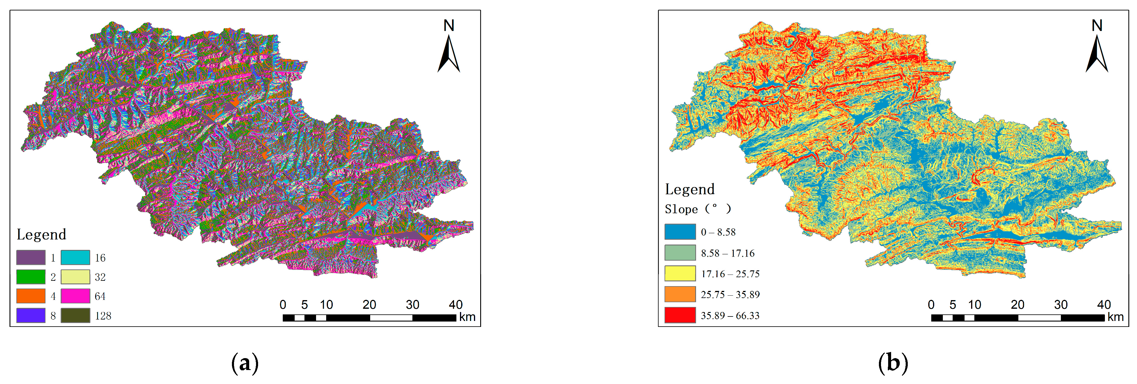
Among the parameters characterizing the land use type, the initial value for the slope element roughness coefficient is determined according to the method of the Liuxihe model, and the evaporation coefficient is set uniformly to 0.7 [31] (Table 3). Soil type parameters include the thickness of soil layer, saturated water content, field moisture retention, wilting moisture content, and saturated hydraulic conductivity. Empirical thickness values for various soil types are shown in Table 4. The soil porosity characteristic, b, is set uniformly to 2.5 [31] for all cells, based on the literature. The saturated water content, field moisture retention, saturated hydraulic conductivity, and wilting moisture content are calculated using the soil hydraulic properties calculator proposed by Arya et al., which was developed by Saxton et al. and can be operated online (“http://www.bsyse.wsu.edu/saxton” (accessed on 15 November 2022)) [40]. Potential evapotranspiration is determined empirically from the climatic conditions of the basin, with one value (0.23 mm/h) applied across the whole catchment. The underground water recession coefficient is set empirically to 0.995. The topographic parameters of flow direction and slope are non-adjustable model parameters calculated from DEM data (Figure 4).

2.4.3. Model Parameter Optimization

The Liuxihe model consists of 13 parameters per unit, which can be classified into four types: meteorological parameters, topographical parameters, soil parameters, and vegetation parameters. Meteorological parameters include potential evapotranspiration, topographical parameters include flow direction and slope, vegetation parameters include evaporation coefficient and slope roughness, and soil parameters include the thickness of soil layer, soil porosity characteristics (b), saturated water content, field moisture retention, wilting moisture content, and saturated hydraulic conductivity. The flow direction and slope are determined using DEM calculation and remain unchanged; they are also known as non-adjustable parameters. Other adjustable parameters are optimized based on initial values using the particle swarm optimization (PSO) algorithm.
In 1995, when American psychologist James Kennedy and electrical engineer Russell Eberhart were studying the diversity of biological populations, they found that birds showed a particular social behavior while hunting. Inspired by this behavior, they proposed the framework of the PSO algorithm [41].
The idea of the PSO algorithm is as follows: Each particle in the algorithm represents a set of parameter solutions. The particle adjusts its velocity and direction by remembering and following the individual and global best positions, thus achieving the optimization process. The particle’s velocity and position transformations are implemented using the following formulas:
V i , k = ω × V i , k 1 + C 1 × r a n d × X i , p B e s t X i , k 1 + C 2 × r a n d × X g B e s t X i , k 1
X i , k = X i , k 1 + V i , k
where V i , k is the velocity of the ith particle at time k, X i , k is the position of the ith particle at time k, X i , p B e s t is the optimal position for individual particle i at time k, X g B e s t is the global optimal position of all particles at time k, ω is the inertia acceleration speed, C 1 and C 2 are learning factors, and r a n d is a random number between 0 and 1.
Meanwhile, the performance of the algorithm can be improved by dynamically adjusting the values of ω . For ω , the linearly decreasing inertia weight strategy (LDIW) proposed by Shi [42] is used for dynamic adjustment in this paper. The calculation formula is as follows:
ω = ω m a x i ω m a x ω m i n M a x N
where i is the current evolution number, M a x N is the maximum evolution number, and ω m a x and ω m i n are the maximum and minimum values of the inertia acceleration speed ω, which are 0.9 and 0.1, respectively.
The Liuxihe model is a distributed model that employs the PSO algorithm for parameter optimization, and the advantage of this model is that data from only one flood are needed for this optimization. Flood 20090607 was selected for model parameter optimization, and the other 24 floods were used for model validation. For PSO algorithm parameter setting, the population size (particle number) of the particle swarm is set to 20. The number of iterations is set to 200, and the total number of calculations is 1000. The inertia factor value range is [0.1, 0.9], with a linear decrease within this range occurring during optimization. The learning acceleration factors C1 and C2 have a value range of [0.5, 2.5] and are optimized dynamically and iteratively within this range according to the anticosine acceleration algorithm. The parameter optimization process and its results are shown in Figure 5.
The results confirm that the optimization effect of parameters obtained using the PSO algorithm is good and that the simulated flood process is consistent with the measured flood process. The peak error for flood 20090607 was reduced from 0.443 to 0.028 after parameter optimization (Table 5). Other evaluation indices verify the high precision and good effect of optimization. Thus, the optimized flood model parameters can be considered to be close to the true values.

3. Results and Discussion

3.1. Flood Simulation Results

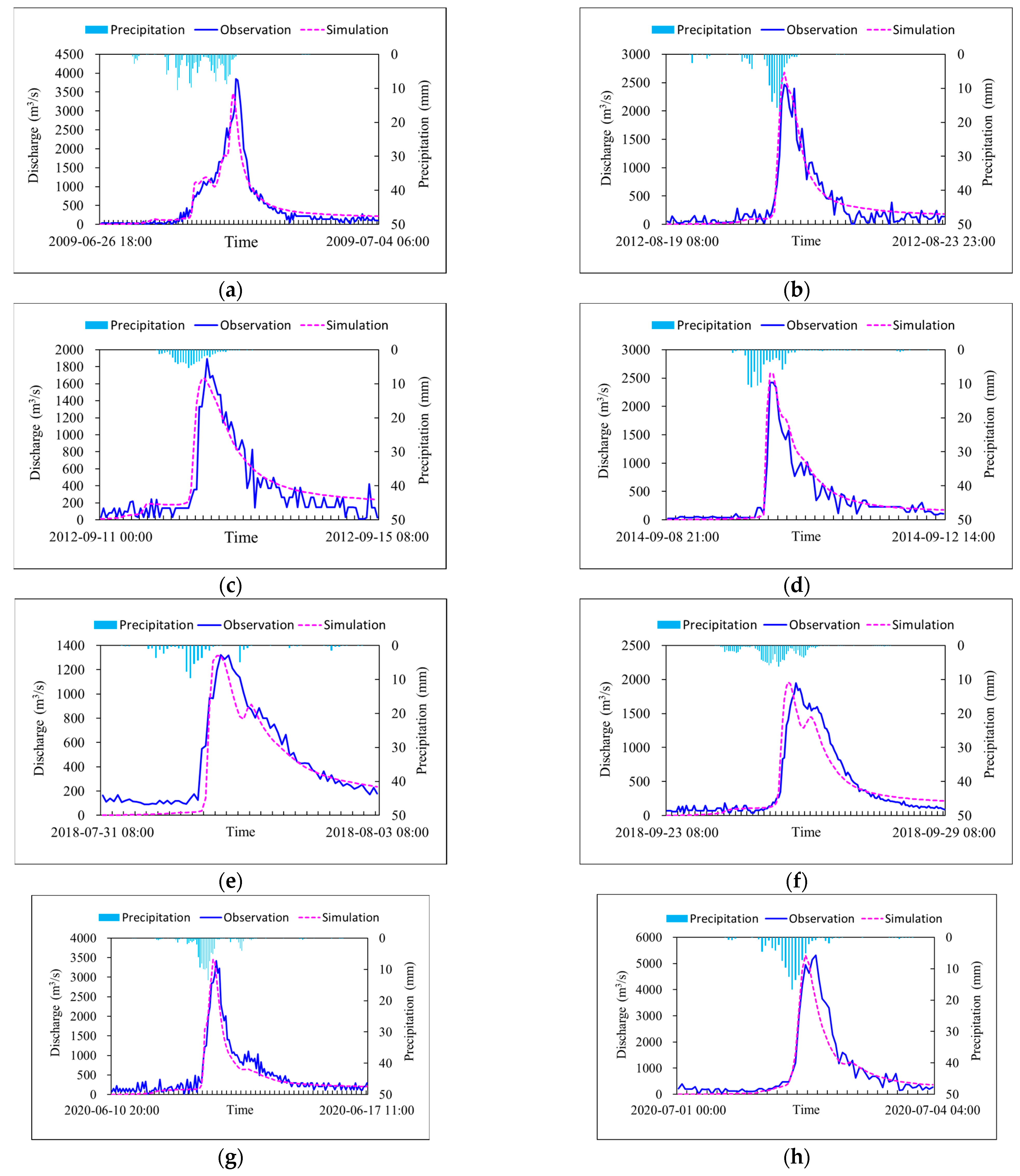
The optimized model parameters were used to simulate the remaining 24 flood processes. Selected simulation results are shown in Figure 6.

3.2. Model Performance Evaluation

In order to quantify the coincidence between measured and simulated flows, six evaluation indices were used: the Nash–Sutcliffe coefficient, correlation coefficient, process relative error, water balance coefficient, peak error, peak time error, and average value. They were calculated using formulas obtained from the literature [43]. The results are provided in Table 6.
With the application of the optimized parameters, the average peak simulation accuracy is 96.3%, the average peak time is 1.042 h early, and the average Nash–Sutcliffe coefficient value is 0.799. Additionally, the simulated flood process curve aligns well with the measured flood process curve. These results demonstrate that the Liuxihe model can simulate floods in a mountainous area accurately to support inflow flood forecasting.

3.3. Simulation to Flood with Uneven Precipitation Spatial Distribution

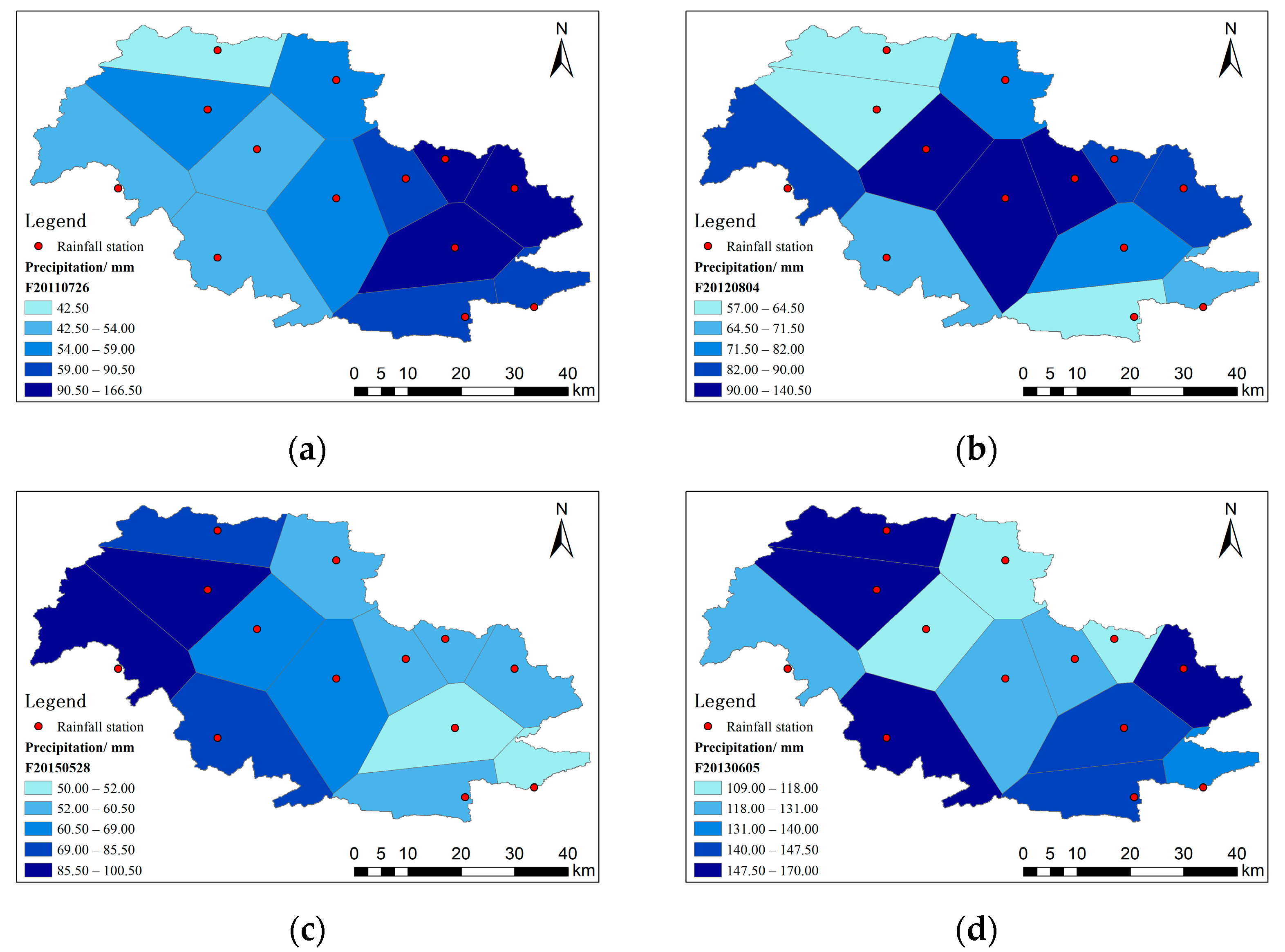
To assess the model’s simulation performance, spatial distribution maps of accumulated rainfall for the 24 floods were drawn and analyzed. The uneven spatial distribution of rainfall (with much more rainfall in some areas than others) is universal and is exhibited by almost every rainfall event. According to their characteristics, the rainfall distributions are divided into four types: downstream, midstream, upstream, and irregular (Figure 7). Four typical floods (one of each type) with extremely uneven spatial rainfall distributions were selected, and their simulation was assessed to verify the applicability of the model as such floods are difficult to simulate using hydrological models.
The simulation results for these four typical floods are shown in Figure 8. The peak accuracies are 99.7%, 98.9%, 99.4%, and 99.7%, respectively. According to the simulation results for the four floods, the Liuxihe model has an excellent simulation effect under the condition of an uneven rainfall distribution, demonstrating the applicability of this distributed hydrological model.

3.4. Analysis of Model Parameter Optimization Results

To explore the influence of the PSO method on the inflow flood simulation accuracy of the Liuxihe model, the optimized and initial parameter values were used for the comparison of 24 floods, and average indicator values for the flood simulation results were obtained. All indicators were significantly improved after parameter optimization (Table 7). Specifically, the average Nash–Sutcliffe coefficient increased by 25.1% from 0.548 to 0.799, the average correlation coefficient increased by 8%, the average process relative error was reduced by 160%, and the average peak error was reduced by 38.8%. Thus, the results show that the PSO algorithm significantly improved the simulation accuracy of the Liuxihe model. This method requires only the selection of a typical flood type for parameter optimization to support practical application, effectively improving the model’s performance.

4. Conclusions

For exploring the effectiveness of the Liuxihe model in real-time flood forecasting for the Zaoshi Reservoir, this study employs a distributed hydrological model, the Liuxihe model, which is based on the DEM, land use data, and soil type data with a resolution of 90 m × 90 m, and uses the PSO algorithm to optimize the model parameters for flood simulation. Using the uneven spatial distributions of flood rainfall, flood prediction for the Zaoshi Reservoir was evaluated. From this study, the following conclusions can be drawn:
  • Each rainfall event analyzed in this paper exhibits an uneven spatial distribution, and the floods can be divided into four types: downstream, midstream, upstream, and irregular.
  • In this study, the Liuxihe model’s flood inflow forecasting scheme for the Zaoshi Reservoir showed an excellent simulation effect, with an average peak simulation accuracy of 96.3%, average peak time of 1.042 h early, and average Nash–Sutcliffe coefficient of 0.799. Under the condition of an uneven spatial distribution of rainfall, the Liuxihe model simulates floods well. Thus, flood simulation with the Liuxihe model is ideal for the watershed above the Zaoshi Reservoir, and the model can be applied in operational flood forecasting.
  • The PSO algorithm significantly improved the simulation precision of the Liuxihe model, and its practical application requires only the selection of a typical flood for parameter optimization, thereby effectively improving the model’s performance.

Author Contributions

Y.C. was responsible for proposing the original idea and providing technical guidance; Y.Z. (Yanzheng Zhu) was responsible for the data compilation, processing, computation, and writing; Y.Z. (Yanjun Zhao), F.Z. and S.X. were responsible for the data sorting. All authors have read and agreed to the published version of the manuscript.

Funding

This study was supported by the National Natural Science Foundation of China (NSFC) (no. 51961125206) and the Science and Technology Program of Guangdong Province (no. 2020B1515120079).

Institutional Review Board Statement

Not applicable.

Informed Consent Statement

Not applicable.

Data Availability Statement

Not applicable.

Conflicts of Interest

The authors declare no conflict of interest.

References

  1. DeVries, B.; Huang, C.; Armston, J.; Huang, W.; Jones, J.W.; Lang, M.W. Rapid and robust monitoring of flood events using Sentinel-1 and Landsat data on the Google Earth Engine. Remote Sens. Environ. 2020, 240, 111664. [Google Scholar] [CrossRef]
  2. Wang, G.; Liu, Y.; Hu, Z.; Lyu, Y.; Zhang, G.; Liu, J.; Liu, Y.; Gu, Y.; Huang, X.; Zheng, H.; et al. Flood risk assessment based on fuzzy synthetic evaluation method in the Beijing-Tianjin-Hebei metropolitan area, China. Sustainability 2020, 12, 1451. [Google Scholar] [CrossRef] [Green Version]
  3. Török, I. Qualitative assessment of social vulnerability to flood hazards in Romania. Sustainability 2018, 10, 3780. [Google Scholar] [CrossRef] [Green Version]
  4. Zhang, M.; Xiang, W.; Chen, M.; Mao, Z. Measuring social vulnerability to flood disasters in China. Sustainability 2018, 10, 2676. [Google Scholar] [CrossRef] [Green Version]
  5. Choi, H.I. Spatial assessment of damage vulnerability to storms based on the analysis of historical damage cost data in the Korean Peninsula. Sustainability 2019, 11, 6051. [Google Scholar] [CrossRef] [Green Version]
  6. Urban, M.C. Accelerating extinction risk from climate change. Science 2015, 348, 571–573. [Google Scholar] [CrossRef] [Green Version]
  7. O’Gorman, P.A. Precipitation extremes under climate change. Curr. Clim. Chang. Rep. 2015, 1, 49–59. [Google Scholar] [CrossRef] [Green Version]
  8. Kabiso, A.F.; O’Neill, E.; Brereton, F.; Abeje, W. Rapid Urbanization in Ethiopia: Lakes as Drivers and Its Implication for the Management of Common Pool Resources. Sustainability 2022, 14, 12788. [Google Scholar] [CrossRef]
  9. Bremard, T. Monitoring land subsidence: The challenges of producing knowledge and groundwater management indicators in the Bangkok metropolitan region, Thailand. Sustainability 2022, 14, 10593. [Google Scholar] [CrossRef]
  10. Huong, H.T.L.; Pathirana, A. Urbanization and climate change impacts on future urban flooding in Can Tho city, Vietnam. Hydrol. Earth Syst. Sci. 2013, 17, 379–394. [Google Scholar] [CrossRef] [Green Version]
  11. Miller, J.D.; Hutchins, M. The impacts of urbanisation and climate change on urban flooding and urban water quality: A review of the evidence concerning the United Kingdom. J. Hydrol. Reg. Stud. 2017, 12, 345–362. [Google Scholar] [CrossRef] [Green Version]
  12. Zhang, K.; Gann, D.; Ross, M.; Robertson, Q.; Sarmiento, J.; Santana, S.; Rhome, J.; Fritz, C. Accuracy assessment of ASTER, SRTM, ALOS, and TDX DEMs for Hispaniola and implications for mapping vulnerability to coastal flooding. Remote Sens. Environ. 2019, 225, 290–306. [Google Scholar] [CrossRef]
  13. Quesada-Román, A. Flood risk index development at the municipal level in Costa Rica: A methodological framework. Environ. Sci. Policy 2022, 133, 98–106. [Google Scholar] [CrossRef]
  14. Chen, C.; Jiang, J.; Zhou, Y.; Lv, N.; Liang, X.; Wan, S. An edge intelligence empowered flooding process prediction using Internet of things in smart city. J. Parallel Distrib. Comput. 2022, 165, 66–78. [Google Scholar] [CrossRef]
  15. Chen, L.; Chen, Y.; Zhang, Y.; Xu, S. Spatial patterns of typhoon rainfall and associated flood characteristics over a mountainous watershed of a tropical island. J. Hydrol. 2022, 613, 128421. [Google Scholar] [CrossRef]
  16. Rui, X. On watershed hydrological model. Adv. Water Conserv. Hydropower Technol. 2017, 37, 1–7+58. [Google Scholar]
  17. Jie, M.X.; Chen, H.; Xu, C.Y.; Zeng, Q.; Tao, X.E. A comparative study of different objective functions to improve the flood forecasting accuracy. Hydrol. Res. 2016, 47, 718–735. [Google Scholar] [CrossRef] [Green Version]
  18. Lu, M. Review and Prospect of Xin’anjiang Model Research. J. Water Resour. 2021, 52, 432–441. [Google Scholar]
  19. Du, J.; Qian, L.; Rui, H.; Zuo, T.; Zheng, D.; Xu, Y.; Xu, C.Y. Assessing the effects of urbanization on annual runoff and flood events using an integrated hydrological modeling system for Qinhuai River basin, China. J. Hydrol. 2012, 464, 127–139. [Google Scholar] [CrossRef]
  20. Freeze, R.A.; Harlan, R.L. Blueprint for a physically-based, digitally-simulated hydrologic response model. J. Hydrol. 1969, 9, 237–258. [Google Scholar] [CrossRef]
  21. Abbott, M.B.; Bathurst, J.C.; Cunge, J.A.; O’Connell, P.E.; Rasmussen, J. An introduction to the European Hydrological System-Systeme Hydrologique Europeen, “SHE”, 2:structure of a physically based, distributed modeling system. J. Hydrol. 1986, 87, 61–77. [Google Scholar] [CrossRef]
  22. Liang, X.; Lettenmaier, D.P.; Wood, E.F.; Burges, S.J. A simple hydrologically based model of land surface water and energy fluxes for general circulation models. J. Geophys. Res. 1994, 99, 14415–14428. [Google Scholar] [CrossRef]
  23. Wang, Z.; Batelaan, O.; Smedt, F.D. A distributed model for water and energy transfer between soil, plants and atmosphere (WetSpa). Phys. Chem. Earth 1996, 21, 189–193. [Google Scholar] [CrossRef]
  24. Vieux, J.; Ceo, P. Vflo™: A real-time distributed hydrologic model. In Proceedings of the 2nd Federal Interagency Hydrologic Modeling Conference, Las Vegas, NV, USA, 28 July–1 August 2002; pp. 1–12. [Google Scholar]
  25. Li, L.; Zhong, M. Structure of LL-Ⅱ distributed rainfall runoff model based on GIS. Hydropower Energy Sci. 2003, 21, 35–38. [Google Scholar]
  26. Chen, Y. Liuxihe Model; Science Press: Beijing, China, 2009; 198p. [Google Scholar]
  27. Wang, D.; Tan, D.; Liu, L. Particle swarm optimization algorithm: An overview. Soft Comput. 2018, 22, 387–408. [Google Scholar] [CrossRef]
  28. Zhang, Y.; Wang, S.; Ji, G. A comprehensive survey on particle swarm optimization algorithm and its applications. Math. Probl. Eng. 2015, 2015, 931256. [Google Scholar] [CrossRef] [Green Version]
  29. Xue, B.; Zhang, M.; Browne, W.N. Particle swarm optimization for feature selection in classification: A multi-objective approach. IEEE Trans. Cybern. 2012, 43, 1656–1671. [Google Scholar] [CrossRef]
  30. Bonyadi, M.R.; Michalewicz, Z. Particle swarm optimization for single objective continuous space problems: A review. Evol. Comput. 2017, 25, 1–54. [Google Scholar] [CrossRef]
  31. Chen, Y.; Ren, Q.; Huang, F.; Xu, H.; Cluckie, I. Liuxihe Model and Its Modeling to River Basin Flood. J. Hydrol. Eng. 2011, 16, 33–50. [Google Scholar] [CrossRef]
  32. Zhou, F.; Chen, Y.; Wang, L.; Wu, S.; Shao, G. Flood forecasting scheme of Nanshui reservoir based on Liuxihe model. Trop. Cyclone Res. Rev. 2021, 10, 106–115. [Google Scholar] [CrossRef]
  33. Li, J.; Hong, A.; Yuan, D.; Jiang, Y.; Zhang, Y.; Deng, S.; Cao, C.; Liu, J.; Chen, Y. Elaborate simulations and forecasting of the effects of urbanization on karst flood events using the improved Karst-Liuxihe model. Catena 2020, 197, 104990. [Google Scholar] [CrossRef]
  34. Yang, T.; Rao, S.; Liao, C.; Zhou, D.; Zhang, Y. Preliminary study on forecast of incoming discharge of Zaoshi Reservoir. Water Technol. Econ. 2017, 23, 58–62. [Google Scholar]
  35. Fiedler, F.R. Simple, practical method for determining station weights using Thiessen polygons and isohyetal maps. J. Hydrol. Eng. 2003, 8, 219–221. [Google Scholar] [CrossRef]
  36. Panigrahy, N.; Jain, S.K.; Kumar, V.; Bhunya, P.K. Algorithms for computerized estimation of Thiessen weights. J. Comput. Civ. Eng. 2009, 23, 239–247. [Google Scholar] [CrossRef]
  37. Zhu, Q.A.; Zhang, W.C.; Zhao, D.Z. Topography-based spatial daily precipitation interpolation by means of PRISM and Thiessen polygon analysis. Sci. Geogr. Sin. 2005, 25, 233–238. [Google Scholar]
  38. O’Callaghan, J.F.; Mark, D.M. The extraction of drainage networks from digital elevation data. Comput. Vis. Graph. Image Process. 1984, 28, 323–344. [Google Scholar] [CrossRef]
  39. Strahler, A.N. Quantitative analysis of watershed geomorphology. Trans.—Am. Geophys. Union 1957, 38, 913–920. [Google Scholar] [CrossRef] [Green Version]
  40. Arya, L.M.; Paris, J.F. A Physicoempirical Model to Predict the Soil Moisture Characteristic from Particle-Size Distribution and Bulk Density Data. Soil Sci. Soc. Am. J. 1981, 45, 1023–1030. [Google Scholar] [CrossRef]
  41. Kennedy, J.; Eberhart, R. Particle swarm optimization. In Proceedings of the ICNN’95-International Conference on Neural Networks, Perth, WA, Australia, 27 November–1 December 1995; Volume 4, pp. 1942–1948. [Google Scholar]
  42. Shi, Y. Particle swarm optimization: Developments, applications and resources. In Proceedings of the 2001 Congress on Evolutionary Computation (IEEE Cat. No. 01TH8546), Seoul, Republic of Korea, 27–30 May 2001; Volume 1, pp. 81–86. [Google Scholar]
  43. Zhao, Y.; Chen, Y.; Zhu, Y.; Xu, S. Evaluating the Feasibility of the Liuxihe Model for Forecasting Inflow Flood to the Fengshuba Reservoir. Water 2023, 15, 1048. [Google Scholar] [CrossRef]
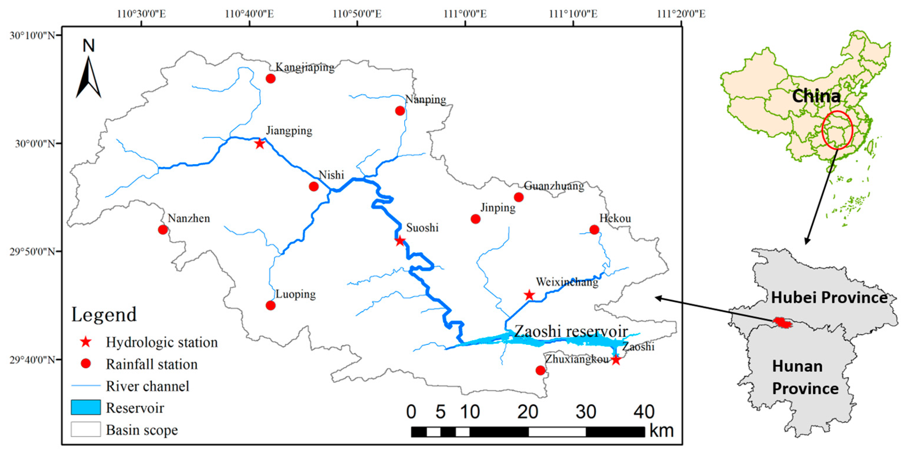
Figure 1. Zaoshi reservoir watershed map.
Sustainability 15 09857 g001
Figure 2. Watershed physical characteristics: (a) DEM, (b) land use, and (c) soil type.
Sustainability 15 09857 g002
Figure 3. Setting of third-order channel segment points in the Liuxihe model.
Sustainability 15 09857 g003
Figure 4. Non-adjustable model parameters of the Zaoshi Reservoir watershed: (a) flow direction and (b) slope.
Sustainability 15 09857 g004
Figure 5. Parameter optimization results: (a) change in the fitness value; (b) changes in parameter values; (c) process curves before and after parameter optimization.
Sustainability 15 09857 g005
Figure 6. Simulation process curves for floods (a) 2009062618, (b) 2012081908, (c) 2012091100, (d) 2014090821, (e) 2018073108, (f) 2018092308, (g) 2020061020, and (h) 2020070100.
Sustainability 15 09857 g006
Figure 7. Rainfall distributions of representative floods (red dots indicate rain gauge locations): (a) downstream type, (b) midstream type, (c) upstream type, and (d) irregular type.
Sustainability 15 09857 g007
Figure 8. Simulation results for four typical uneven spatial distributions of rainfall: (a) flood 2011072600, downstream type; (b) flood 2012080400, midstream type; (c) flood 2015052800, upstream type; and (d) flood 2013060500, irregular type.
Sustainability 15 09857 g008aSustainability 15 09857 g008b
Table 1. Measured flood information.
Flood Event No.Duration (h)Total Rainfall (mm)Peak Discharge (m3/s)
2009060796110.50 2293
20090626181167.31 3842
201005038868.58 1147
201106137391.35 2111
2011061778186.85 8622
201107267277.96 1200
2012062596159.35 3235
2012080412087.08 1764
20120819112109.12 2462
2012091110562.15 1890
2013060596139.23 5010
201307207587.04 2361
20130923120141.15 2334
201407247766.27 1190
201409089087.92 2417
20141027119193.31 3269
201505289668.08 1641
2016061897180.46 4222
201606269180.00 2568
201807317358.42 1321
20180923145114.50 1948
201905249779.08 1354
20200610160119.00 3423
2020070177115.46 5312
20200704103182.88 4588
Table 2. Statistical table for channel order division.
OrderFA0Number of Channel CellsProportion of Channel Cells (%)
62543,93711.9
518716,5784.5
468188112.4
3430037151.0
225,68214580.4
168,2749950.3
Table 3. Parameters of land use type.
Land Use TypeEvaporation CoefficientSlope Roughness Coefficient
Evergreen coniferous forest0.70.4
Evergreen broad-leaved forest0.70.6
Shrubs0.70.4
Thin forest0.70.3
Cultivated land0.70.15
Table 4. Parameters of soil type.
Soil TypeThickness of Soil Layer (mm)Saturated
Water Content
Field Moisture RetentionSaturated Hydraulic ConductivitySoil Porosity CharacteristicsWilting Moisture Content
CN1005110000.5080.4112.192.50.28
CN301159000.4490.2617.272.50.137
CN3011910000.5090.3874.712.50.231
CN3013911400.4950.3853.362.50.244
CN3014913000.4290.21124.132.50.132
CN301517500.4810.3545.32.50.207
CN301735800.4340.22222.712.50.132
CN3017911900.4820.339.852.50.158
CN301935500.4580.22137.342.50.082
CN301996300.4910.4161.042.50.293
CN3025511000.5380.442.172.50.326
CN4004513000.4460.27213.182.50.154
CN5002515500.460.25224.892.50.104
CN601657500.4650.353.912.50.219
CN603157000.4770.29918.082.50.099
Table 5. Simulation evaluation indices for flood 20090607 before and after parameter optimization.
Nash–Sutcliffe CoefficientCorrelation CoefficientProcess
Relative Error
Peak ErrorWater Balance
Coefficient
Peak Time
Error
Before optimization0.7460.9381.2120.4430.911−1
After optimization0.9540.9790.3730.0280.946−2
Table 6. Flood simulation index values.
Flood Event Serial
Number
Nash–Sutcliffe CoefficientCorrelation CoefficientProcess Relative ErrorPeak ErrorWater Balance CoefficientPeak Time Error
20090626 0.8990.9560.7330.0971.017−2
20100503 0.7850.9030.6750.0151.054−3
20110613 0.8390.9380.6440.0281.097−2
20110617 0.8810.9440.4420.010.86−1
20110726 0.7640.8821.0220.0031.077−2
20120625 0.7370.8740.5740.0121.0720
20120804 0.6410.8851.6990.0111.2220
20120819 0.9180.9641.9520.0871.0740
20120911 0.8410.9261.4310.121.153−1
20130605 0.920.960.4960.0030.935−3
20130720 0.8520.940.5850.0071.2312
20130923 0.9210.960.7610.0681.028−2
20140724 0.6410.8711.3880.0041.255−1
20140908 0.9040.9720.4580.0671.1341
20141027 0.9410.9720.5280.0810.9940
201505280.4590.8581.6130.0061.452−3
20160618 0.6280.8371.9040.0631.115−2
20160626 0.8670.9450.2980.0150.87−3
20180731 0.8710.9540.4180.0030.8430
20180923 0.8780.9380.5020.0060.948−4
201905240.4740.7820.5110.0150.701−3
202006100.910.9610.4420.0080.849−2
20200701 0.9020.9560.4960.00010.878−3
20200704 0.6980.9240.350.1540.7219
Average value0.799 0.921 0.830 0.0371.024 −1.042
Table 7. Average indicator values.
Average
Nash–Sutcliffe Coefficient
Average
Correlation Coefficient
Average
Process
Relative Error
Average
Peak Error
Average
Water Balance
Coefficient
Average
Peak Time
Error
Initial model parameter 0.548 0.841 2.430 0.425 1.076 −0.167
Optimized parameter0.799 0.921 0.830 0.0371.024 −1.042
Disclaimer/Publisher’s Note: The statements, opinions and data contained in all publications are solely those of the individual author(s) and contributor(s) and not of MDPI and/or the editor(s). MDPI and/or the editor(s) disclaim responsibility for any injury to people or property resulting from any ideas, methods, instructions or products referred to in the content.