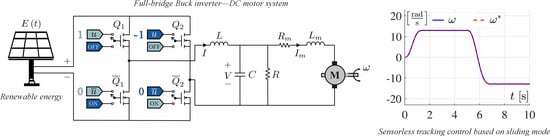
Sensorless Tracking Control Based on Sliding Mode for the “Full-Bridge Buck Inverter–DC Motor” System Fed by PV Panel

Abstract

This paper presents a sliding mode control (SMC) for the “full-bridge Buck inverter–DC motor” system when a photovoltaic (PV) panel is considered as the power supply. The control executes the trajectory tracking task related to the angular velocity of the DC motor shaft without the need for electromechanical sensors. The proposed control is validated through realistic simulation results via Matlab-Simulink. In this regard, the system is constructed by using the electronic components of the specialized power systems library of Simscape. The results of the following four case studies are presented: (i) The performance of the closed-loop system considering two desired angular velocity profiles and three different incident solar irradiance shapes on the PV panel. (ii) An analysis associated with the primary energy source. (iii) A comparison of the proposed SMC versus a passive control. (iv) A study of the current ripple and its relationship with the execution of the tracking control task on the angular velocity.

1. Introduction

The generation of electric energy has led to numerous environmental issues due to over-exploitation of natural resources [1]. Because of this, the industrial sector has adopted, as an alternative, the utilization of some resources that can be continuously regenerated with the aim of generating electric energy. In this context, systems that take advantage of solar irradiance have been developed with the purpose of generating electric energy. Such systems are commonly known as photovoltaic (PV) panels and have found widespread applications in various fields such as lighting, domotics [2], generation of movement and agriculture [3], among others. In this regard, generation of movement is greatly exploited by electric machines when energy is generated through solar irradiance. However, when electric machines are fed through this kind of energy, the power supply has to be capable of being self-adaptable to the voltage variations that commonly arise in PV panels due to environmental conditions. An alternative to attenuating such variations is through the implementation of a DC/DC electronic converter at the output of the PV panel with the objective of generating a robust voltage when environmental variations appear. At the industrial level, DC/DC power electronic converters have been used to control DC motors because some processes require high precision. In the literature, several studies have tackled the control of “DC/DC electronic converter–DC motor” systems, where the regulation and the angular velocity tracking tasks have been solved. Within these works, researchers have addressed both the problem of unidirectional rotation and the problem of bidirectional rotation associated with the DC motor shaft. As a result, the following section presents an overview of the current state of the art regarding these issues.

1.1. Unidirectional Systems

Nowadays, several topologies of DC/DC electronic converters have been proposed and constructed with the objective of providing a unipolar output voltage. Consequently, when these converters are connected to a DC motor, they generate unidirectional rotation of the motor shaft. In this regard, the following papers describe topologies that are commonly used as unidirectional drivers for DC motors.

1.1.1. DC/DC Buck Converter Driven DC Motor

For this system, the following contributions have been reported. In [4], Lyshevsky developed a nonlinear PI control. In [5], Ahmad et al. designed and compared the performance of PI control, fuzzy PI, and linear quadratic regulator (LQR) algorithms. On the other hand, papers [6,7,8] focused on control strategies based on differential flatness for solving the tracking task. In [9], Bingöl and Paçaci developed software for controlling the DC/DC Buck power converter through neural networks. In [10], Sira-Ramírez and Oliver-Salazar reported the concepts of differential flatness and active disturbance rejection in DC/DC Buck converters connected to DC motors. Meanwhile, Hoyos et al. in [11,12,13,14] applied the zero average dynamic technique and the fixed-point induction control for controlling the angular velocity of the Buck converter–DC motor combination. Likewise, in [15,16,17,18,19], active disturbance rejection schemes were developed for controlling the angular velocity of DC motors driven by a DC/DC Buck converter, while in [20], Guerrero-Ramírez et al. also proposed an active disturbance rejection control and added a PV panel, as the power supply, for feeding the Buck converter connected to a DC motor for solving the regulation task. On the other hand, a sliding mode control (SMC) scheme was presented by Silva-Ortigoza et al. and Wei et al. in [21,22], respectively. In this regard, Xiao et al. in [23] used an SMC along with a proton exchange membrane fuel cell power as a renewable energy power source for the DC/DC Buck converter–DC motor system. Moreover, Rauf et al. studied SMC in [24,25], while Ravikumar and Srinivasan implemented a high-order SMC in [26]. In a different direction, Khubalkar et al. in [27,28,29] tuned some fractional order PID controllers through dynamic particle swarm optimization (dPSO), via an improvement of dPSO, and by using the ant colony optimization concept, respectively. Recently, some other control techniques have been investigated; for example, the piecewise affine PI-based control proposed by Hanif et al. in [30], the neuroadaptive backstepping-based control, the intelligent nonlinear adaptive control, and a neural network-based intelligent control developed by Nizami et al. in [31,32,33], respectively; an adaptive neurofuzzy H_∞-based control designed by Rigatos et al. in [34], the fault detection control algorithm based on a switching observer with the bond graph method introduced by Kazemi and Montazeri in [35], and the exact tracking error dynamics passive output feedback (ETEDPOF) methodology presented by Srinivasan et al. in [36,37]. Finally, a continuous control implemented via PWM and an SMC with chattering elimination were presented in [38,39], respectively.

1.1.2. Other DC/DC Converter Topologies for Driving a DC Motor

Papers exploring the implementation of the Boost topology as a driver for a DC motor are provided here. Linares-Flores et al. designed a passivity-based control in [40] for solving the angular velocity trajectory tracking task. On the other hand, Alexandridis and Konstantopoulos implemented a modified PI controller for DC motors fed by DC/DC Boost converters in [41] and an improved control technique in [42]. Likewise, Malek presented a new design of a nonlinear robust control in [43], while Mishra et al. developed a digital PWM-based control for a DC/DC Boost converter connected to a permanent magnet DC motor in [44]. Govindharaj and Mariappan, in [45], designed a neural adaptive backstepping controller for the angular velocity trajectory tracking task. In another direction, Alajami et al. in [46] implemented a PI controller for electric vehicle motors that are powered by a DC/DC Boost converter. Moreover, the performance of a two-loop PI controller for a DC/DC Boost converter that drives a permanent magnet DC motor was analyzed in [47]. Lastly, in [48], Silva-Ortigoza et al. presented a hierarchical control based on flatness that considers the dynamics of the power supply derived from solar energy.

Papers focusing on the implementation of the Buck–Boost topology in driving DC motors are described here. Sönmez and Dursun in [49] proposed and implemented a current control based on fuzzy logic for the DC/DC Buck–Boost converter in connection with a DC motor and the obtained results were compared to a classic PI control. For the same system, Linares-Flores et al. in [50] developed a robust control scheme based on passivity. Recently, Gurumoorthy and Balaraman designed in [51] an SMC for a PV system (based on a Buck–Boost converter) that powers a DC motor.

For the Luo converter, Srinivasan et al. in [52] introduced a passivity-based control and estimation of the load torque when the Luo converter considers a dynamic load.

The cascaded combination of the Cuk converter with a DC motor was controlled in [53] via a hierarchical control based on differential flatness and SMC.

The multilevel Buck topology was studied by Ismail and Elnady in [54] with the aim of attenuating the current and torque waves generated by the abrupt changes in the Buck converter. Likewise, an angular velocity control based on active disturbance rejection was reported by Guerrero et al. in [55] for the parallel DC/DC Buck converter–DC motor system.

1.2. Bidirectional Systems

Configurations of DC/DC electronic converters delivering a bipolar output voltage generate a bidirectional rotation in the motor shaft. In the following, the state-of-the-art review linked to topologies commonly used as bidirectional drivers for DC motors is presented.

1.2.1. Bidirectional DC/DC Buck Converter Driven DC Motor

With the purpose of carrying out bidirectional rotation in the shaft of a DC motor fed by a DC/DC Buck converter, two approaches have been proposed where an inverter circuit is utilized. In [56], the mathematical model of the full-bridge Buck inverter–DC motor system was developed and experimentally validated. Additionally, with the aim of solving the trajectory tracking task in such a system, Silva-Ortigoza et al. designed a sensorless control based on the ETEDPOF methodology and a robust control based on the differential flatness concept in [57,58], respectively. In [59], Hernández-Márquez et al. implemented a robust tracking control strategy based on differential flatness. Furthermore, Chi et al. presented an adaptive tracking SMC with neural network estimation related to the estimation of the Chebyshev neural network in [60]. On the other hand, in addition to what has been presented in this section, some studies that have addressed the control strategies for the full-bridge Buck inverter are the works presented in [61,62,63,64].

1.2.2. Other Bidirectional DC/DC Converter Topologies for Driving a DC Motor

A differential flatness control strategy for the DC/DC Boost converter–inverter–DC motor system was proposed in [65]. In addition, Egidio et al. in [66] proposed an integral control strategy for the angular velocity and the angular position of a DC motor connected to a DC/DC Boost converter–inverter.

For the Buck–Boost topology, in [67], Hernández-Márquez et al. designed a hierarchical robust control for trajectory tracking. Meanwhile, in [68], Ghazali et al. performed a Neuroendocrine-PID control for MIMO systems. The Sepic topology was examined in [69], where Linares-Flores et al. developed a sensorless control strategy based on passivity for the full-bridge Sepic converter–DC motor system powered by a solar energy source.

1.3. Discussion of Related Works

In accordance with the above, different DC/DC converter topologies connected to a DC motor, as well as various control schemes that solve the regulation and trajectory tracking tasks, are proposed in Section 1.1 and Section 1.2. However, there are few contributions where renewable energy sources are considered. For example, in [8], Silva-Ortigoza et al. approximated the behavior of a Topsun TS-S425 PV panel using a programmable TDK-Lambda G100-17 power supply, which was responsible for powering a DC/DC Buck converter–DC motor system. They applied a control algorithm based on differential flatness and solved the trajectory tracking task. On the other hand, in [20], Guerrero-Ramírez et al. developed an active disturbance rejection control for solving the regulation task for the DC/DC Buck converter–DC motor system while being powered by a PV panel. Additionally, Xiao et al. implemented an SMC for the DC/DC Buck converter–DC motor system powered by proton exchange membrane fuel cell power in [23]. A common feature among these contributions is their ability to enable the unidirectional rotation of the motor shaft. This property is exploited in a variety of applications; for instance, in [70], Koksal developed a hybrid control scheme for a mechatronic system using a DC/DC Buck converter as a voltage regulator. Meanwhile, applications in wheeled mobile robots were studied by García-Sánchez et al. in [71].

In contrast, studies that incorporate renewable energy sources and address bidirectional rotation of the motor shaft include the work by Linares-Flores et al. in [69], who tackled the regulation problem using a passivity-based control strategy and a DC/DC Sepic converter–inverter connected to a DC motor powered by a PV panel. Another study by Chi et al. in [60] utilized an adaptive SMC with neural network estimation and a proton exchange membrane fuel cell-powered source as the renewable energy source for a DC/DC Buck inverter–DC motor system. Furthermore, in the literature, studies have been presented where the primary power source is generated from renewable energy that feeds power electronic converters or other systems. Within these contributions, the following applications are found: power converters [72,73,74], AC motors [75,76], pumping systems [77,78,79], and electric vehicle motors [80,81,82].

1.4. Contribution

Based on the above, it is clear that there is a lack of proposals using renewable energy sources to supply a power electronic converter connected to a DC motor for addressing the bidirectional trajectory tracking task. Therefore, this research aims to develop an SMC scheme to achieve the trajectory tracking task in the full-bridge Buck inverter–DC motor system, which demonstrates an optimal performance even in the presence of supply voltage fluctuations caused by variations in solar irradiation on the panel due to environmental factors. It is important to mention that the implementation of the proposed controller eliminates the need for electromechanical sensors. With the intention of highlighting the contributions associated with this work, the following are listed:

i.

For the first time in the literature, a sensorless tracking SMC is proposed for the full-bridge Buck inverter–DC motor system, which considers the dynamics of the power supply in the control design. The performance of the SMC is verified in Section 4 for two reference trajectories, when the feeding voltage is time-varying and when it is generated through a PV panel considering three different solar irradiance shapes.

ii.

The power supply operating range is determined in Section 5.1. This allows one to determine the minimum voltage magnitude that the power supply must provide in order to achieve the control task. Results of the system in closed-loop with different PV panels that satisfy the power supply operating range are presented for this purpose.

iii.

A performance comparison between the proposed SMC and an ETEDPOF control is conducted in Section 5.2. This demonstrates the superiority of the proposed SMC in terms of trajectory tracking performance.

iv.

A study related to current ripple and trajectory tracking assessment is presented in Section 5.3. This establishes the dependency between the SMC implementation frequency and the current ripple. Additionally, it is inferred that as the current ripple decreases, the performance of the control task improves.

1.5. Work Organization

The remaining sections of the paper are focused on the following. Section 2 presents the generalities of the model associated with the full-bridge Buck inverter–DC motor system fed by a PV panel. In Section 3, the design of the SMC for the trajectory tracking task is shown and the stability analysis in closed-loop is presented using the Lyapunov approach. Simulation results of the system in closed-loop, considering two desired velocities and three different solar irradiance shapes incident on the PV panel, are depicted in Section 4. Section 5 focuses on three different studies associated with the system: (a) an analysis of the valid operating range for the power supply, (b) a comparison between the proposed SMC and an ETEDPOF control, and (c) an analysis of the current ripple in relation to the execution of the tracking control task. Finally, conclusions and future works are given in Section 6.

2. Full-Bridge Buck Inverter–DC Motor System

In this section, the mathematical model that defines the dynamic behavior of the full-bridge Buck inverter–DC motor system is presented.

Figure 1 shows the electromechanical diagram of the full-Bridge Buck inverter–DC motor system. This system consists of a power supply $E\left(t\right)$, a set of four transistors $Q_1,{\overline{Q}}_1,Q_2$ and ${\overline{Q}}_2$ that operate according to the duty cycles described in Figure 1, a low-pass filter $LC$ which provides a continuous output voltage V at the terminals of the capacitor C and the load resistance R, and I is the current that flows through the inductor L. The output voltage V powers a DC motor, which has parameters such as armature current $I_m$ flowing through armature resistance $R_m$ and armature inductance $L_m$, while the parameters associated with its mechanical design are the moment of inertia J, the coefficient of viscous friction b, the motor torque constant $k_m$, and the back-electromotive force constant $k_e$. Finally, $\omega$ corresponds to the angular velocity of the motor shaft.

According to [56], the switched mathematical model of the full-bridge Buck inverter–DC motor system in Figure 1 is given by:

$$\begin{array}{cc}\hfill L\frac{dI}{dt}& =-V+E\left(t\right)u,\hfill \\ \hfill C\frac{dV}{dt}& =I-\frac{V}{R}-I_m,\hfill \\ \hfill L_m\frac{d{I}_m}{dt}& =V-R_m{I}_m-k_e\omega ,\hfill \\ \hfill J\frac{d\omega }{dt}& =k_m{I}_m-b\omega ,\hfill \end{array}$$

(1)

where $u\in \{-1,0,1\}$ represents the position of transistors $Q_1,{\overline{Q}}_1,Q_2$, and ${\overline{Q}}_2$ in accordance with the duty cycle shown in Figure 1. The average mathematical model of the full-bridge Buck inverter–DC motor is [56]:

$$\begin{array}{cc}\hfill L\frac{dI}{dt}& =-V+E\left(t\right)u_{av},\hfill \\ \hfill C\frac{dV}{dt}& =I-\frac{V}{R}-I_m,\hfill \\ \hfill L_m\frac{d{I}_m}{dt}& =V-R_m{I}_m-k_e\omega ,\hfill \\ \hfill J\frac{d\omega }{dt}& =k_m{I}_m-b\omega ,\hfill \end{array}$$

(2)

where $u_{av}\in [-1,1]$ is the average duty cycle of the input signal. The mathematical model (2) can be represented in the form $\dot{x}=f\left(x\right)+g\left(x\right)u_{av}$ as follows:

$$\underset{\dot{x}}{\underbrace{\left[\begin{array}{c}\dot{I}\\ \dot{V}\\ {\dot{I}}_m\\ \dot{\omega }\end{array}\right]}}=\underset{f\left(x\right)}{\underbrace{\left[\begin{array}{c}-\frac{V}{L}\\ \frac{1}{C}\left(I-\frac{V}{R}-I_m\right)\\ \frac{1}{L_m}\left(V-R_m{I}_m-k_e\omega \right)\\ \frac{1}{J}\left(K_m{I}_m-b\omega \right)\end{array}\right]}}+\underset{g\left(x\right)}{\underbrace{\left[\begin{array}{c}\frac{E\left(t\right)}{L}\\ 0\\ 0\\ 0\end{array}\right]}}{u}_{av}.$$

(3)

The representation (3) will be used for designing the control strategy. Based on [56], the average mathematical model (2) is differentially flat and can be represented in terms of $\omega$ and its successive time derivatives. Therefore, considering a desired angular velocity profile ${\omega }^{*}$ and (2), the reference trajectories of the system, i.e., $I^{*}$, $V^{*}$, $I_m^{*}$, and $u_{av}^{*}$, are determined by the following equations:

$$\begin{array}{cc}\hfill u_{av}^{*}& =\left(\frac{CJL{L}_m}{k_{m}E\left(t\right)}\right){\omega }^{*\left(4\right)}+\left(\frac{bCL{L}_{m}R+CJLR{R}_m+JL{L}_m}{k_{m}RE\left(t\right)}\right){\stackrel{⃛}{\omega }}^{*}\hfill \\ & +\left(\frac{J{L}_{m}R+L\left(L_{m}b+JR+J{R}_m+CR\left(R_{m}b+k_e{k}_m\right)\right)}{k_{m}RE\left(t\right)}\right){\ddot{\omega }}^{*}\hfill \\ \hfill & +\left(\frac{bLR+bL{R}_m+b{L}_{a}R+k_e{k}_{m}L+JR{R}_a}{k_{m}RE\left(t\right)}\right){\dot{\omega }}^{*}+\left(\frac{b{R}_m+k_e{k}_m}{k_{m}E\left(t\right)}\right){\omega }^{*},\hfill \end{array}$$

(4)

$$\begin{array}{cc}\hfill I^{*}& =\left(\frac{J{L}_{m}C}{k_m}\right){\stackrel{⃛}{\omega }}^{*}+\left(\frac{L_{m}J+RC\left(b{L}_m+J{R}_m\right)}{R{k}_m}\right){\ddot{\omega }}^{*}\hfill \\ & +\left(\frac{L_{m}b+JR+J{R}_m+RC\left(k_e{k}_m+R_{m}b\right)}{k_{m}R}\right){\dot{\omega }}^{*}+\left(\frac{k_e{k}_m+R_{m}b+Rb}{k_{m}R}\right){\omega }^{*},\hfill \end{array}$$

(5)

$$\begin{array}{cc}\hfill V^{*}& =\left(\frac{J{L}_m}{k_m}\right){\ddot{\omega }}^{*}+\left(\frac{b{L}_m+J{R}_m}{k_m}\right){\dot{\omega }}^{*}+\left(\frac{k_e{k}_m+R_{m}b}{k_m}\right){\omega }^{*},\hfill \end{array}$$

(6)

$$\begin{array}{cc}\hfill I_m^{*}& =\left(\frac{J}{k_m}\right){\dot{\omega }}^{*}+\left(\frac{b}{k_m}\right){\omega }^{*}.\hfill \end{array}$$

(7)

In this work, the following parameters for the full-bridge Buck inverter were considered:

$$\begin{array}{c}L=4.94\mathrm{mH},C=4.7\mathsf{\mu }\mathrm{F},R=48\mathrm{\Omega }.\end{array}$$

(8)

The parameters of the DC motor are:

$$\begin{array}{c}{L}_m=2.22\mathrm{mH},R_m=0.965\mathrm{\Omega },k_m=120.1\times {10}^{-3}\frac{\mathrm{N}·\mathrm{m}}{\mathrm{A}},\hfill \\ k_e=120.1\times {10}^{-3}\frac{\mathrm{V}·\mathrm{s}}{\mathrm{rad}},J=118.2\times {10}^{-3}\mathrm{kg}·{\mathrm{m}}^2,b=129.6\times {10}^{-3}\frac{\mathrm{N}·\mathrm{m}·\mathrm{s}}{\mathrm{rad}}.\hfill \end{array}$$

(9)

3. Sensorless Tracking Control Based on Sliding Mode Design

This section presents the design of the sensorless tracking control based on sliding mode for solving the trajectory tracking task on the full-bridge Buck inverter–DC motor system. To accomplish this, first the design of a direct control (i.e., a control that allows $\omega \to {\omega }^{*}$) is presented. Then, an indirect control that does not make use of electromechanical sensors is developed.

3.1. Direct Control

A sliding surface for proposing a direct control over the angular velocity $\omega$ is the following:

$$h\left(x,t\right)=\omega -{\omega }^{*}.$$

(10)

The directional derivative of function $h\left(x,t\right)$ in direction $f\left(x\right)$ is:

$$L_{f}h\left(x,t\right)=\frac{\partial h\left(x,t\right)}{\partial x}\left[\begin{array}{c}-\frac{V}{L}\\ \frac{1}{C}\left(I-\frac{V}{R}-I_m\right)\\ \frac{1}{L_m}\left(V-R_m{I}_m-k_e\omega \right)\\ \frac{1}{J}\left(K_m{I}_m-b\omega \right)\end{array}\right]=\frac{1}{J}\left(k_m{I}_m-b\omega \right),$$

(11)

whereas the directional derivative of function $h\left(x,t\right)$ in direction $g\left(x\right)$ is:

$$L_{g}h\left(x,t\right)=\frac{\partial h\left(x,t\right)}{\partial x}\left[\begin{array}{c}\frac{E\left(t\right)}{L}\\ 0\\ 0\\ 0\end{array}\right]=0.$$

(12)

In [83], Sira-Ramírez demonstrated that the equivalent control can be found through the following equation:

$$u_{eq}=-\frac{L_{f}h\left(x,t\right)}{L_{g}h\left(x,t\right)}-\frac{\partial h\left(x,t\right)}{\partial t}\left(\frac{1}{L_{g}h\left(x,t\right)}\right).$$

(13)

Based on (11)–(13), the sliding surface defined through (10) is not viable, since $u_{eq}\to \pm \infty$.

3.2. Indirect Control

Since it is not possible to establish a sliding surface involving the angular velocity $\omega$, an indirect control is proposed to perform the angular velocity tracking task by manipulating the electric current I. In this regard, the following sliding surface is proposed:

$$h\left(x,t\right)=I-I^{*}.$$

(14)

Now, the directional derivative of function $h\left(x,t\right)$ in direction $f\left(x\right)$ is:

$$L_{f}h\left(x,t\right)=\frac{\partial h\left(x,t\right)}{\partial x}\left[\begin{array}{c}-\frac{V}{L}\\ \frac{1}{C}\left(I-\frac{V}{R}-I_m\right)\\ \frac{1}{L_m}\left(V-R_m{I}_m-k_e\omega \right)\\ \frac{1}{J}\left(K_m{I}_m-b\omega \right)\end{array}\right]=-\frac{V}{L},$$

(15)

while the directional derivative of function $h\left(x,t\right)$ in direction $g\left(x\right)$ is:

$$L_{g}h\left(x,t\right)=\frac{\partial h\left(x,t\right)}{\partial x}\left[\begin{array}{c}\frac{E\left(t\right)}{L}\\ 0\\ 0\\ 0\end{array}\right]=\frac{E\left(t\right)}{L}.$$

(16)

Hence, and in accordance with (13) and (15)–(16), the equivalent control is given by:

$$u_{eq}=\frac{1}{E\left(t\right)}\left(V+L\frac{d{I}^{*}}{dt}\right).$$

(17)

To analyze the closed-loop dynamic behavior of the system, the control law $u_{eq}$ (17) is introduced into the average input signal $u_{av}$ of the model (2). Thus, the ideal sliding dynamics are obtained, which are given by the following subsystem of differential equations:

$$\begin{array}{cc}\hfill C\frac{dV}{dt}& =I^{*}-\frac{V}{R}-I_m,\hfill \\ \hfill L_m\frac{d{I}_m}{dt}& =V-R_m{I}_m-k_e\omega ,\hfill \\ \hfill J\frac{d\omega }{dt}& =k_m{I}_m-b\omega .\hfill \end{array}$$

(18)

Now, the tracking errors $e_1$, $e_2$, and $e_3$ associated with the state variables $V,I_m$, and $\omega$, respectively, are defined as:

$$\begin{array}{cc}\hfill e_1& =V-V^{*},\hfill \\ \hfill e_2& =I_m-I_m^{*},\hfill \\ \hfill e_3& =\omega -{\omega }^{*}.\hfill \end{array}$$

(19)

Thus, after using (19), the ideal sliding dynamics (18) expressed in terms of the tracking errors is,

$$\begin{array}{cc}\hfill C\frac{d{e}_1}{dt}& =-\frac{1}{R}{e}_1-e_2,\hfill \\ \hfill L_m\frac{d{e}_2}{dt}& =e_1-R_m{e}_2+k_e{e}_3,\hfill \\ \hfill J\frac{d{e}_3}{dt}& =k_m{e}_2-b{e}_3.\hfill \end{array}$$

(20)

With the aim of verifying the stability of the system in closed-loop, the error dynamics given by (20) and the following definite positive candidate Lyapunov function proposal are used,

$$\vartheta \left(e_1,e_2,e_3\right)=\frac{1}{2}C{e}_1^2+\frac{1}{2}{L}_m{e}_2^2+\frac{1}{2}J{e}_3^2>0.$$

The first derivative with respect to time of the definite positive candidate Lyapunov function, along the regulation error dynamics, gives as a result:

$$\begin{array}{c}\dot{\vartheta }\left(e_1,e_2,e_3\right)=C{\dot{e}}_1{e}_1+L_m{\dot{e}}_2{e}_2+J{\dot{e}}_3{e}_3=-\left(\frac{1}{R}{e}_1^2+R_m{e}_2^2+b{e}_3^2\right)<0,\hfill \end{array}$$

which guarantees that the system in closed-loop is asymptotically stable. Hence, the sliding surface (14) achieves that $I\to I^{*}$ through the following switched control signal:

$$u=\left\{\begin{array}{cc}1\hfill & h(x,t)\le 0\hfill \\ -1\hfill & h(x,t)>0.\hfill \end{array}\right.$$

(21)

4. Simulation Results 1: Closed-Loop System Performance

In order to validate the performance of the proposed control strategy, this section presents closed-loop simulation results for the full-bridge Buck inverter–DC motor system. Here, the following are considered:

• A time-varying supply voltage from a PV panel.
• Three different forms of solar irradiation (constant, sinusoidal, and stochastic).
• Two different reference trajectories (one of Bézier type and the other of sinusoidal type).

For these simulations, a Topsun TS-S410 PV panel was used, whose technical specifications are shown in

Table 1. Characteristics of the Topsun TS - S410 PV panel.

Characteristics	Magnitude
Maximum power ($P_{max}$)	410.108 W
Voltage at maximum power ($V_{max}$)	50.32 V
Current at maximum power ($I_{max}$)	8.15 A
Open circuit voltage ($V_{oc}$)	61.06 V
Short circuit current ($I_{sc}$)	8.77 A

.

Figure 2 shows two graphs. The first one depicts the dependence between the current and the output voltage of the panel, while the second one presents the relationship between the power and the output voltage of the PV panel. In both graphs, $I_r\in \left\{500,800,1000,1200\right\}$ is considered.

Figure 3 presents the block diagram to numerically simulate the closed-loop dynamic behavior of the full-bridge Buck inverter–DC motor system powered by a PV panel. The blocks that compose the diagram in Figure 3 are the following:

• Sliding mode control. The SMC scheme is implemented in this block in Simulink. The reference trajectory ${\omega }^{*}$ is defined by the block labeled desired velocity. This desired trajectory is used to calculate the reference variables $I^{*}$, $V^{*}$, and $I_m^{*}$ using Equation (5). On the other hand, the control block requires the measurement of the current I and the reference variable $I^{*}$, with which the control signal u is determined in accordance with Equation (21). Finally, through the control implementation block, the control signal is established for the transistors $Q_1,{\overline{Q}}_1,Q_2$, and ${\overline{Q}}_2$, based on the duty cycles shown in Figure 1.
• Full-bridge Buck inverter–DC motor circuit. This block corresponds to the Matlab-Simulink development of the full-bridge Buck inverter–DC motor system shown in Figure 1. The power source is a Topsun TS-S410 PV panel that is subjected to time-varying solar irradiation $I_r$, which produces a time-varying power supply voltage $E\left(t\right)$. In this electromechanical circuit, the variables I, V, $I_m$, and $\omega$ are measured. While the parameter values associated with the Buck converter and DC motor used to simulate the closed-loop system are presented in (8) and (9), respectively.

For the simulations presented here, two reference trajectories for the angular velocity ${\omega }^{*}$ have been proposed. The first desired trajectory is defined by two Bézier polynomials, selected as follows:

$${\omega }^{*}\left(t\right)=\left\{\begin{array}{c}{\overline{\omega }}_{i_1}\left(t_{i_1}\right)+[{\overline{\omega }}_{f_1}\left(t_{f_1}\right)-{\overline{\omega }}_{i_1}\left(t_{i_1}\right)]{\phi }_1\left(t,t_{i_1},t_{f_1}\right)t\le 3\mathrm{s},\hfill \\ {\overline{\omega }}_{i_2}\left(t_{i_2}\right)+[{\overline{\omega }}_{f_2}\left(t_{f_2}\right)-{\overline{\omega }}_{i_2}\left(t_{i_2}\right)]{\phi }_2\left(t,t_{i_2},t_{f_2}\right)t>3\mathrm{s},\hfill \end{array}\right.$$

(22)

where ${\phi }_1\left(t,t_{i_1},t_{f_1}\right)$ and ${\phi }_2\left(t,t_{i_2},t_{f_2}\right)$ are Bézier polynomials defined as:

$$\begin{array}{c}\hfill {\phi }_1=\left\{\begin{array}{c}0t\le t_{i_1},\hfill \\ {\varsigma }_1^3[20-45{\varsigma }_1+36{\varsigma }_1^2-10{\varsigma }_1^3]t\in (t_{i_1},t_{f_1}),\hfill \\ 1t\ge t_{f_1},\hfill \end{array}\right.\end{array}$$

$$\begin{array}{c}\hfill {\phi }_2=\left\{\begin{array}{c}0t\le t_{i_2},\hfill \\ {\varsigma }_2^3[20-45{\varsigma }_1+36{\varsigma }_1^2-10{\varsigma }_1^3]t\in (t_{i_2},t_{f_2}),\hfill \\ 1t\ge t_{f_2},\hfill \end{array}\right.\end{array}$$

${\varsigma }_1=\frac{t-t_{i_1}}{t_{f_1}-t_{i_1}}$, ${\varsigma }_2=\frac{t-t_{i_2}}{t_{f_2}-t_{i_2}}$, $t_{i_1}=0\mathrm{s}$, $t_{f_1}=1.5\mathrm{s}$, $t_{i_2}=5\mathrm{s}$, $t_{f_2}=7\mathrm{s}$, ${\overline{\omega }}_{i_1}=0\frac{\mathrm{rad}}{\mathrm{s}}$, ${\overline{\omega }}_{f_1}=13\frac{\mathrm{rad}}{\mathrm{s}}$, ${\overline{\omega }}_{i_2}=13\frac{\mathrm{rad}}{\mathrm{s}}$ and ${\overline{\omega }}_{f_2}=-13\frac{\mathrm{rad}}{\mathrm{s}}$.

The second desired trajectory for ${\omega }^{*}$ is selected as:

$${\omega }^{*}\left(t\right)=10sin\left(0.8\pi t\right).$$

(23)

In the following, three simulation results are presented to show the behavior of the full-bridge Buck inverter–DC motor system for an angular velocity profile ${\omega }^{*}$ given by (22), considering three different solar irradiance conditions, denoted as $I_r$. Here and throughout this work (unless otherwise stated), the switching frequency to be considered in the simulations, via the sampling time, will be $f=500\mathrm{kHz}$.

4.1. Simulation Test 1

The simulation presented here assumes the following constant magnitude of incident solar irradiation, $I_r$, on the PV panel:

$$I_r=1000.$$

(24)

The simulation results of this test are depicted in Figure 4.

4.2. Simulation Test 2

To test the performance of the control scheme under varying input voltage conditions, a sinusoidal time-varying solar irradiation is considered in this simulation:

$$I_r=100sin\left(10t\right)+900.$$

(25)

Figure 5 shows the results of this simulation.

4.3. Simulation Test 3

To validate the robustness of the controller against abrupt changes in the input voltage, a solar irradiation with random changes every $0.7$ seconds within the following interval is proposed:

$$I_r\in \left[800,1200\right].$$

(26)

The corresponding results of this simulation are shown in Figure 6.

In order to illustrate the performance of the controller when periodic reference signals are considered, three new simulations are presented with a sinusoidal reference trajectory (23), which again uses three solar irradiation behaviors $I_r$.

4.4. Simulation Test 4

For this test, a solar irradiance $I_r$ incident on the panel of constant magnitude (24) is defined. The simulation results are shown in Figure 7.

4.5. Simulation Test 5

In this simulation, a periodic solar irradiance $I_r$ given by (25) is considered. The results of this test are displayed in Figure 8.

4.6. Simulation Test 6

The closed-loop system dynamics are shown in Figure 9 when random changes in solar irradiation are considered every 0.7 seconds within the interval given by (26).

4.7. Comments of the Simulation Results

The simulation results presented in Figure 4, Figure 5, Figure 6, Figure 7, Figure 8 and Figure 9 demonstrate that the proposed SMC for the full-bridge Buck inverter–DC motor system achieves the trajectory tracking task, i.e., $\omega \to {\omega }^{*}$. It is worth noting that the implemented control scheme regulates the angular velocity through the feedback of the current flowing through the inductor. Next, we briefly analyze the results associated with simulation tests 4–6.

In simulation test 1, a constant solar irradiation $I_r$ (24) and a Bézier-type angular velocity profile (22) were established. Figure 4 shows that good trajectory tracking was achieved on $\omega$ despite the voltage drops in $E\left(t\right)$ caused by the increase in current demand.

On the other hand, Figure 5 presents the results of simulation test 2. For this simulation, a time-varying solar irradiation $I_r$ (25) was set, causing fluctuations in the input voltage of the inverter $E\left(t\right)$. However, the controller shows good performance, i.e., $\omega \to {\omega }^{*}$.

In simulation test 3, a solar irradiation $I_r$ is considered, which presents unexpected changes in magnitude every 0.7 seconds that are reflected in the input voltage of the converter $E\left(t\right)$. Figure 6 shows that despite the abrupt changes in the input voltage, the controller is able to maintain the angular velocity on its desired trajectory.

Finally, in simulation tests 4–6, a sinusoidal velocity profile (23) is established and tests are performed for cases of constant (24), sinusoidal (25), and random (26) solar irradiation. In each of these tests, the performance of the designed SMC for the full-bridge Buck inverter–DC motor system was verified, as the angular velocity converges to the reference value ${\omega }^{*}$. The obtained simulation results demonstrate the robustness and effectiveness of the proposed SMC scheme, as it can effectively compensate for the disturbances caused by the varying solar irradiation and maintain accurate tracking of the desired velocity trajectory. Overall, the presented simulation tests validate the suitability of the proposed control strategy for the considered full-bridge Buck inverter–DC motor system.

5. Simulation Results 2: System Performance with Different PV Panels, Comparison of the Proposed Control versus an ETEDPOF Control, and Considerations on the SMC Switching Frequency

In this section, new simulations are presented to verify the good performance of the proposed control. First, the minimum voltage magnitude for the power supply $E\left(t\right)$ is determined to ensure the successful execution of the control task associated with $\omega$. Subsequently, a performance comparison is presented between the proposed SMC and a passivity-based control. Finally, the current ripple of I and its impact on trajectory tracking performance are considered when the SMC switching frequency is taken into account.

5.1. Power Supply Operating Range Analysis

Starting from Equation (4), after considering the maximum voltage transfer point from the full-bridge Buck inverter to the motor (i.e., $u_{av}^{*}=1$), the following expression is obtained for $E\left(t\right)$ in terms of ${\omega }^{*}\left(t\right)$,

$$\begin{array}{cc}\hfill E\left(t\right)& =\left(\frac{CJL{L}_m}{k_m}\right){\omega }^{*\left(4\right)}+\left(\frac{bCL{L}_{m}R+CJLR{R}_m+JL{L}_m}{k_{m}R}\right){\stackrel{⃛}{\omega }}^{*}\hfill \\ & +\left(\frac{J{L}_{m}R+L\left(L_{m}b+JR+J{R}_m+CR\left(R_{m}b+k_e{k}_m\right)\right)}{k_{m}R}\right){\ddot{\omega }}^{*}\hfill \\ \hfill & +\left(\frac{bLR+bL{R}_m+b{L}_{m}R+k_e{k}_{m}L+JR{R}_m}{k_{m}R}\right){\dot{\omega }}^{*}+\left(\frac{b{R}_m+k_e{k}_m}{k_m}\right){\omega }^{*}.\hfill \end{array}$$

(27)

From (27), after considering a desired trajectory ${\omega }^{*}$ and obtaining the $\max |{\omega }^{*}|$, it is determined that the minimum magnitude required for $E\left(t\right)$ must satisfy the following constraint,

$$E\left(t\right)\ge \left(\frac{b{R}_m+k_e{K}_m}{k_m}\right)\max \left|{\omega }^{*}\right|.$$

(28)

By applying (28) to the sinusoidal reference trajectory (23), the following is obtained:

$$E\left(t\right)\ge 11.6143\mathrm{V}.$$

(29)

Now, by choosing a PV panel that provides a $V_{oc}$ lower than the one studied in Section 4, it is shown how the fulfillment of (29) achieves $\omega \to {\omega }^{*}$ for constant, sinusoidal, and random irradiations given by (24)–(26), respectively. Thus, an appropriate selection for the PV panel is achieved by proposing the use of an Aleo Solar S59Y310, whose technical specifications are presented in

Table 2. Aleo Solar S59Y310 PV panel characteristics.

Characteristics	Magnitude
Maximum power ($P_{max}$)	310.66 W
Voltage at maximum power ($V_{max}$)	31.7 V
Current at maximum power ($I_{max}$)	9.8 A
Open circuit voltage ($V_{oc}$)	39.7 V
Short circuit current ($I_{sc}$)	10.12 A

.

Considering the incident solar irradiation $I_r$ (24), the sinusoidal angular velocity profile ${\omega }^{*}$ (23), and the Aleo Solar S59Y310 PV panel, the simulation results depicted in Figure 10 are obtained.

Now, considering the time-varying sinusoidal solar irradiation $I_r$ (25), the results presented in Figure 11 are obtained.

By applying the random solar irradiation $I_r$ (26), and once again using the desired angular velocity ${\omega }^{*}$ (23), the dynamics shown in Figure 12 is obtained.

On the other hand, in order to verify the performance of the system with PV panels that have open-circuit voltages $V_{oc}$ higher than the one discussed in Section 4 and satisfy the constraint (29), a NuvoSun FL1132-440 PV panel is considered as the power source. The technical specifications of this PV panel are shown in

Table 3. NuvoSun FL1132-440 PV panel characteristics.

Characteristics	Magnitude
Maximum power ($P_{max}$)	$440.118$ W
Voltage at maximum power ($V_{max}$)	$88.2$ V
Current at maximum power ($I_{max}$)	$4.99$ A
Open circuit voltage ($V_{oc}$)	$112.4$ V
Short circuit current ($I_{sc}$)	$5.66$ A

. Next, three new simulations are presented under constant, sinusoidal, and random irradiations given by (24)–(26), respectively. Here, a sinusoidal reference angular velocity profile ${\omega }^{*}$ (23) is considered once again.

The following simulation considers the reference angular velocity profile ${\omega }^{*}$ (23) and the constant solar irradiation $I_r$ (24). The obtained results are shown in Figure 13.

For the simulation depicted in Figure 14, the reference angular velocity ${\omega }^{*}$ given by (23) and $I_r$ given by (25) are considered.

Finally, the results of the closed-loop system considering the desired angular velocity (23) and solar irradiation (26) are presented in Figure 15.

5.2. Comparison of the SMC versus a Sensorless ETEDPOF Control

In order to verify the superiority of the SMC strategy designed in this paper, a comparison is now presented between this strategy and a passivity-based control [57]. Since the SMC (21) only requires the use of the electric current I, no mechanical sensors such as tachometers or encoders are needed for its implementation. Therefore, in order to be impartial, a velocity sensorless control based on the ETEDPOF methodology, developed for the full-bridge Buck inverter–DC motor system in [57], was selected. Such a control scheme is defined as follows:

$$u_{av}=-\gamma E\left(t\right)(I_P-I^{*})+u_{av}^{*},$$

(30)

where $I_P$ represents the current flowing through the inductor L (i.e., $I_P=I$), while $\gamma$ represents the sensorless tracking control gain, and $u_{av}^{*}$ corresponds to the nominal trajectory associated with the input, given by (4). On the other hand, $E\left(t\right)$ corresponds to the power supply, as previously explained, produced via PV panels. Finally, $I^{*}$ was defined earlier in (5). Note that the control signal (30), as well as the sliding surface (14) associated with the proposed SMC, entirely depend on the measurement of the current $I_P$ flowing through the inductor L. Therefore, for both control strategies, if $I\to I^{*}$, then $\omega \to {\omega }^{*}$ accordingly. To perform the comparison between the SMC (21) and the ETEDPOF control (30), it is now appropriate to define the tracking errors for the state variables I and $\omega$. For the SMC, the current tracking error, $e_I$ and the angular velocity tracking error, $e_{\omega }$, are defined as follows:

$$e_I=I-I^{*},$$

(31)

$$e_{\omega }=\omega -{\omega }^{*}.$$

(32)

Note that (32) was previously defined in (19) for the stability analysis of the closed-loop system with the SMC. Here, it has been redefined as the tracking error of $\omega$ associated with the SMC (21). Meanwhile, for the ETEDPOF control, the current tracking error, $e_{I_P}$, and the angular velocity tracking error, $e_{{\omega }_P}$, are defined by the following equations:

$$e_{I_P}=I_P-I^{*},$$

(33)

$$e_{{\omega }_P}={\omega }_P-{\omega }^{*},$$

(34)

where ${\omega }_P$ is the angular velocity obtained from the closed-loop system when considering the ETEDPOF control (30). Regarding the sensorless tracking control gain $\gamma$ associated with (30), in the following three simulation results, $\gamma =0.003$ is considered (as in [57]).

Based on the above, after considering $E\left(t\right)$ from the Topsun TS-S425 PV panel used in Section 4 (see Table 1), three different simulation tests related to constant, sinusoidal, and random irradiations given by (24)–(26), respectively, are presented. Consequently, the graphical results illustrate the dynamic evolution of the variables I, $I_P$, $\omega$, and ${\omega }_P$ associated with their tracking errors $e_I$, $e_{I_P}$, $e_{\omega }$, and $e_{{\omega }_P}$, respectively.

Considering the sinusoidal reference trajectory ${\omega }^{*}$ (23) and the constant solar irradiation $I_r$ (24), Figure 16 shows the comparative simulation results associated with the states I, $I_P$, $\omega$, and ${\omega }_P$, as well as the errors $e_I$, $e_{I_P}$, $e_{\omega }$, and $e_{{\omega }_P}$.

For the next simulation test, the same sinusoidal function ${\omega }^{*}$ given by (23) is considered, along with $I_r$ given by (25). The behavior of the system controlled via the ETEDPOF methodology, as compared to the system under the SMC, is shown in Figure 17.

Finally, the result illustrated in Figure 18 concerns a random solar irradiation $I_r$ (26) with the desired angular velocity profile ${\omega }^{*}$ (23).

5.3. Dependency of f in the SMC: Evaluation of Current Ripple and Trajectory Tracking Performance

Here, the study related to the current ripple associated with I, flowing through the inductor L, resulting from applying the SMC (21) to the full-bridge Buck inverter–DC motor system, is presented. In order to conduct this study, new simulation results are presented, considering different switching frequencies for the transistors that compose the inverter circuit. Based on these new results, the trajectory tracking task is assessed.

The switching frequencies associated with the implementation of the SMC (21) that are proposed to visualize the current ripple associated with I and the tracking performance associated with $\omega$ are $f=50\mathrm{kHz}$, $250\mathrm{kHz}$, and $500\mathrm{kHz}$. Under these considerations for f, ${\omega }^{*}$ defined by (23), and $I_r$ given by (26), the corresponding results are illustrated in Figure 19. In this figure, $I_{{50}_{kHz}}$ and ${\omega }_{{50}_{kHz}}$, $I_{{250}_{kHz}}$ and ${\omega }_{{250}_{kHz}}$, and $I_{{500}_{kHz}}$ and ${\omega }_{{500}_{kHz}}$ denote the results associated with the frequencies $f=50\mathrm{kHz}$, $250\mathrm{kHz}$, and $500\mathrm{kHz}$, respectively, for I and $\omega$.

In Figure 19, it can be observed that at $f=50\mathrm{kHz}$, there is a pronounced ripple in $I_{{50}_{kHz}}$ and a significant tracking error in the angular velocity variable, ${\omega }_{{50}_{kHz}}$. On the other hand, at $f=250\mathrm{kHz}$, the ripple in $I_{{250}_{kHz}}$ and the tracking error in ${\omega }_{{250}_{kHz}}$ are smaller compared to those observed at $f=50\mathrm{kHz}$. Finally, at $f=500\mathrm{kHz}$, the ripple in the variable $I_{{500}_{kHz}}$ is barely noticeable and there is good tracking performance in the angular velocity ${\omega }_{{500}_{kHz}}$. Therefore, it can be inferred that as the switching frequency in the transistors of the full-bridge Buck inverter–DC motor system increases, the ripple in I decreases. Consequently, the tracking performance on the angular velocity variable $\omega$ improves, achieving that $\omega \to {\omega }^{*}$.

5.4. Comments on the Simulation Results

In this section, a summary of the findings encountered during the development of this section is presented. These findings are based on the obtained simulation results. As a synthesis, the following comments are given for each of the three points studied in this section:

• Power supply operating range analysis. After analyzing the simulation results obtained in Section 5.1 and presented in Figure 10, Figure 11, Figure 12, Figure 13, Figure 14 and Figure 15, it is demonstrated that the system exhibits good performance even when using PV panels with different technical characteristics. This is due to the fact that the panels used in these simulations consistently satisfy condition (28). It is worth noting that despite the sudden variations in the incident solar irradiation on the panel, the good performance of the control remains.
• Comparison of the SMC versus a sensorless ETEDPOF control. In Figure 16, Figure 17 and Figure 18 presented in Section 5.2, the superiority of the proposed SMC is evident. This is because the tracking errors associated with the variables I (see Figure 16c, Figure 17c, and Figure 18c) and $\omega$ (see Figure 16d, Figure 17d, and Figure 18d) are smaller in magnitude compared to the errors obtained via the ETEDPOF control.
• Dependency of f in the SMC: Current Ripple and Trajectory Tracking Task Assessment. In Section 5.3, after visually evaluating the results presented in Figure 19, it can be concluded that the performance of the SMC is directly dependent on its switching frequency. This is evident as a higher frequency leads to a decrease in the current ripple present in I and an improvement in the tracking performance of $\omega$, i.e., if ideally $f\to \infty$, then $e_{\omega }\to 0$.

Lastly, another point worth highlighting for the system under study is the performance of sensitivity analysis, which would help determine the state variable that is most sensitive to variations in a specific parameter of interest in the system. However, in our work, we do not perform a sensitivity analysis since the mathematical model of the bidirectional system studied here is very similar to the dynamic model of the unidirectional “DC/DC Buck converter–DC motor system”. The sensitivity analysis for the latter system has already been reported in detail in [37]. It was demonstrated there that the inductor current I is considered as the sensitive variable. Furthermore, a passive control based on the ETEDPOF methodology was developed, in which the sensitive variable is inherently used in such a control strategy (as is the case in the ETEDPOF control (30), reported in [57]). Similarly, in [37] it is concluded that due to the current being the more sensitive variable, which coincides with the feedback variable in the ETEDPOF strategy, it enables the controller to outperform other controllers such as PI control.

6. Conclusions

The focus of this work was to develop a sensorless SMC strategy for the full-bridge Buck inverter–DC motor system. It was found that it is not feasible to implement this control directly on the output variable of interest, i.e., $\omega$. Therefore, an indirect control approach based on the current I flowing in the inductor of the Buck inverter was designed. Since the system is differentially flat, the differential parametrization was used to define the reference trajectory $I^{*}$ in terms of the desired angular velocity profile ${\omega }^{*}$. Furthermore, the stability of the closed-loop system was verified using Lyapunov’s theory. Simulation results clearly demonstrate that the control objective, i.e., $I\to I^{*}$ and consequently $\omega \to {\omega }^{*}$, is achieved even when there are variations in the input voltage due to abrupt changes in the solar irradiation incident on the PV panel. Indeed, the proposed sensorless SMC strategy for the full-bridge Buck inverter–DC motor system has shown to be effective in using renewable energy sources such as a PV panel to power a DC motor. In general, this work provides a promising approach for efficient and reliable control of DC motors using renewable energy sources. The above is supported by the results obtained in closed-loop in Section 4. On the other hand, from the results obtained in Section 5, the following findings are also obtained:

• The restriction relating the desired angular velocity ${\omega }^{*}$ to the minimum required magnitude of $E\left(t\right)$ to successfully perform the control task was found.
• It was demonstrated that the performance of the proposed SMC is better than a control based on the ETEDPOF methodology.
• It was shown that as the current ripple in I decreases, the trajectory tracking task is improved. This is achieved by increasing the frequency in the SMC implementation.

Finally, based on the findings presented in this paper, future works could focus on the experimental validation of the proposed SMC, taking into account the high switching frequency associated with the control. Additionally, the application of other types of renewable energy sources to power this system could be explored. This could involve investigating the feasibility and performance of using wind, hydroelectric or other forms of solar energy (such as concentrated solar power) to drive the DC motor through the full-bridge Buck inverter. Furthermore, conducting a budget error analysis would be beneficial as a future work.

References

1. Obaideen, K.; Olabi, A.G.; Al Swailmeen, Y.; Shehata, N.; Abdelkareem, M.A.; Alami, A.H.; Rodriguez, C.; Sayed, E.T. Solar energy: Applications, trends analysis, bibliometric analysis and research contribution to sustainable development goals (SDGs). Sustainability 2023, 15, 1418. [Google Scholar] [CrossRef]
2. Elkholy, M.H.; Senjyu, T.; Lotfy, M.E.; Elgarhy, A.; Ali, N.S.; Gaafar, T.S. Design and implementation of a real-time smart home management system considering energy saving. Sustainability 2022, 14, 13840. [Google Scholar] [CrossRef]
3. Zainol Abidin, M.A.; Mahyuddin, M.N.; Mohd Zainuri, M.A.A. Solar photovoltaic architecture and agronomic management in agrivoltaic system: A review. Sustainability 2021, 13, 7846. [Google Scholar] [CrossRef]
4. Lyshevski, S.E. Electromechanical Systems, Electric Machines and Applied Mechatronics; CRC Press: Boca Raton, FL, USA, 2000; ISBN 0-8493-2275-8. [Google Scholar]
5. Ahmad, M.A.; Ismail, R.M.T.R.; Ramli, M.S. Control strategy of Buck converter driven DC motor: A comparative assessment. Austral. J. Basic Appl. Sci. 2010, 4, 4893–4903. [Google Scholar]
6. Rigatos, G.; Siano, P.; Wira, P.; Sayed-Mouchaweh, M. Control of DC–DC converter and DC motor dynamics using differential flatness theory. Intell. Ind. Syst. 2016, 2, 371–380. [Google Scholar] [CrossRef] [Green Version]
7. Rigatos, G.; Siano, P.; Ademi, S.; Wira, P. Flatness-based control of DC-DC converters implemented in successive loops. Electr. Power Compon. Syst. 2018, 46, 673–687. [Google Scholar] [CrossRef]
8. Silva-Ortigoza, R.; Roldán-Caballero, A.; Hernández-Márquez, E.; García-Sánchez, J.R.; Marciano-Melchor, M.; Hernández-Guzmán, V.M.; Silva-Ortigoza, G. Robust flatness tracking control for the “DC/DC Buck converter–DC motor” system: Renewable energy-based power supply. Complexity 2021, 2021, 2158782. [Google Scholar] [CrossRef]
9. Bingöl, O.; Paçaci, S. A virtual laboratory for neural network controlled DC motors based on a DC-DC Buck converter. Int. J. Eng. Educ. 2012, 28, 713–723. [Google Scholar]
10. Sira-Ramírez, H.; Oliver-Salazar, M.A. On the robust control of Buck-converter DC-motor combinations. IEEE Trans. Power Electron. 2013, 28, 3912–3922. [Google Scholar] [CrossRef]
11. Hoyos, F.E.; Rincón, A.; Taborda, J.A.; Toro, N.; Angulo, F. Adaptive quasi-sliding mode control for permanent magnet DC motor. Math. Probl. Eng. 2013, 2013, 693685. [Google Scholar] [CrossRef] [Green Version]
12. Hoyos Velasco, F.E.; Candelo-Becerra, J.E.; Rincón Santamaria, A. Dynamic analysis of a permanent magnet DC motor using a Buck converter controlled by ZAD-FPIC. Energies 2018, 11, 3388. [Google Scholar] [CrossRef] [Green Version]
13. Hoyos, F.E.; Candelo-Becerra, J.E.; Hoyos Velasco, C.I. Application of zero average dynamics and fixed point induction control techniques to control the speed of a DC motor with a Buck converter. Appl. Sci. 2020, 10, 1807. [Google Scholar] [CrossRef] [Green Version]
14. Hoyos, F.E.; Candelo-Becerra, J.E.; Rincón, A. Zero average dynamic controller for speed control of DC motor. Appl. Sci. 2021, 11, 5608. [Google Scholar] [CrossRef]
15. Yang, J.; Wu, H.; Hu, L.; Li, S. Robust predictive speed regulation of converter-driven DC motors via a discrete-time reduced-order GPIO. IEEE Trans. Ind. Electron. 2019, 66, 7893–7903. [Google Scholar] [CrossRef] [Green Version]
16. Stanković, M.R.; Madonski, R.; Shao, S.; Mikluc, D. On dealing with harmonic uncertainties in the class of active disturbance rejection controllers. Int. J. Control 2021, 94, 2795–2810. [Google Scholar] [CrossRef]
17. Madonski, R.; Łakomy, K.; Stankovic, M.; Shao, S.; Yang, J.; Li, S. Robust converter-fed motor control based on active rejection of multiple disturbances. Control Eng. Pract. 2021, 107, 104696. [Google Scholar] [CrossRef]
18. Zhang, L.; Yang, J.; Li, S. A model-based unmatched disturbance rejection control approach for speed regulation of a converter-driven DC motor using output-feedback. IEEE-CAA J. Autom. Sin. 2022, 9, 365–376. [Google Scholar] [CrossRef]
19. Guerrero-Ramírez, E.; Martínez-Barbosa, A.; Guzmán-Ramírez, E.; Barahona-Ávalos, J.L. Design methodology for digital active disturbance rejection control of the DC motor drive. E-Prime-Adv. Electr. Eng. Electron. Energy 2022, 2, 100050. [Google Scholar]
20. Guerrero-Ramírez, E.; Martínez-Barbosa, A.; Contreras-Ordaz, M.A.; Guerrero-Ramírez, G.; Guzman-Ramirez, E.; Barahona-Ávalos, J.L.; Adam-Medina, M. DC motor drive powered by solar photovoltaic energy: An FPGA-based active disturbance rejection control approach. Energies 2022, 15, 6595. [Google Scholar] [CrossRef]
21. Silva-Ortigoza, R.; Hernández-Guzmán, V.M.; Antonio-Cruz, M.; Muñoz-Carrillo, D. DC/DC Buck power converter as a smooth starter for a DC motor based on a hierarchical control. IEEE Trans. Power Electron. 2015, 30, 1076–1084. [Google Scholar] [CrossRef]
22. Wei, F.; Yang, P.; Li, W. Robust adaptive control of DC motor system fed by Buck converter. Int. J. Control Autom. 2014, 7, 179–190. [Google Scholar] [CrossRef]
23. Xiao, X.; Lv, J.; Chang, Y.; Chen, J.; He, H. Adaptive sliding mode control integrating with RBFNN for proton exchange membrane fuel cell power conditioning. Appl. Sci. 2022, 12, 3132. [Google Scholar] [CrossRef]
24. Rauf, A.; Li, S.; Madonski, R.; Yang, J. Continuous dynamic sliding mode control of converter-fed DC motor system with high order mismatched disturbance compensation. Trans. Inst. Meas. Control 2020, 42, 2812–2821. [Google Scholar] [CrossRef]
25. Rauf, A.; Zafran, M.; Khan, A.; Tariq, A.R. Finite-time nonsingular terminal sliding mode control of converter-driven DC motor system subject to unmatched disturbances. Int. Trans. Elect. Energy Syst. 2021, 31, e13070. [Google Scholar] [CrossRef]
26. Ravikumar, D.; Srinivasan, G.K. Implementation of higher order sliding mode control of DC–DC Buck converter fed permanent magnet DC motor with improved performance. Automatika 2022, 64, 162–177. [Google Scholar] [CrossRef]
27. Khubalkar, S.; Chopade, A.; Junghare, A.; Aware, M.; Das, S. Design and realization of stand-alone digital fractional order PID controller for Buck converter fed DC motor. Circuits Syst. Signal Process. 2016, 35, 2189–2211. [Google Scholar] [CrossRef]
28. Khubalkar, S.W.; Junghare, A.S.; Aware, M.V.; Chopade, A.S.; Das, S. Demonstrative fractional order – PID controller based DC motor drive on digital platform. ISA Trans. 2018, 82, 79–93. [Google Scholar] [CrossRef]
29. Patil, M.D.; Vadirajacharya, K.; Khubalkar, S.W. Design and tuning of digital fractional-order PID controller for permanent magnet DC motor. IETE J. Res. 2021, 1–11. [Google Scholar] [CrossRef]
30. Hanif, M.I.F.M.; Suid, M.H.; Ahmad, M.A. A piecewise affine PI controller for Buck converter generated DC motor. Int. J. Power Electron. Drive Syst. 2019, 10, 1419–1426. [Google Scholar] [CrossRef]
31. Nizami, T.K.; Chakravarty, A.; Mahanta, C. Design and implementation of a neuro-adaptive backstepping controller for Buck converter fed PMDC-motor. Control Eng. Pract. 2017, 58, 78–87. [Google Scholar] [CrossRef]
32. Nizami, T.K.; Chakravarty, A.; Mahanta, C.; Iqbal, A.; Hosseinpour, A. Enhanced dynamic performance in DC–DC converter-PMDC motor combination through an intelligent non-linear adaptive control scheme. IET Power Electron. 2022, 15, 1607–1616. [Google Scholar] [CrossRef]
33. Nizami, T.K.; Gangula, S.D.; Reddy, R.; Dhiman, H.S. Legendre neural network based intelligent control of DC-DC step down converter-PMDC motor combination. IFAC 2022, 55, 162–167. [Google Scholar] [CrossRef]
34. Rigatos, G.; Siano, P.; Sayed-Mouchaweh, M. Adaptive neurofuzzy H-infinity control of DC-DC voltage converters. Neural Comput. Appl. 2020, 33, 2507–2520. [Google Scholar] [CrossRef]
35. Kazemi, M.G.; Montazeri, M. Fault detection of continuous time linear switched systems using combination of bond graph method and switching observer. ISA Trans. 2019, 94, 338–351. [Google Scholar] [CrossRef] [PubMed]
36. Kumar, S.G.; Thilagar, S.H. Sensorless load torque estimation and passivity based control of Buck converter fed DC motor. Sci. World J. 2015, 2015, 132843. [Google Scholar] [CrossRef] [Green Version]
37. Srinivasan, G.K.; Srinivasan, H.T.; Rivera, M. Sensitivity analysis of exact tracking error dynamics passive output control for a flat/partially flat converter Systems. Electronics 2020, 9, 1942. [Google Scholar] [CrossRef]
38. Shneen, S.W.; Shuraiji, A.L.; Hameed, K.R. Simulation model of proportional integral controller-PWM DC-DC power converter for DC motor using matlab. Indones. J. Electr. Eng. Comput. Sci. 2023, 29, 725–734. [Google Scholar] [CrossRef]
39. Chouya, A. Adaptive sliding mode control with chattering elimination for Buck converter driven DC motor. WSEAS Trans. Syst. Control 2023, 22, 19–28. [Google Scholar] [CrossRef]
40. Linares-Flores, J.; Reger, J.; Sira-Ramírez, H. Load torque estimation and passivity-based control of a Boost-converter/DC-motor combination. IEEE Trans. Control Syst. Technol. 2010, 18, 1398–1405. [Google Scholar] [CrossRef]
41. Alexandridis, A.T.; Konstantopoulos, G.C. Modified PI speed controllers for series-excited DC motors fed by DC/DC Boost converters. Control Eng. Pract. 2014, 23, 14–21. [Google Scholar] [CrossRef]
42. Konstantopoulos, G.C.; Alexandridis, A.T. Enhanced control design of simple DC-DC Boost converter-driven DC motors: Analysis and implementation. Electr. Power Compon. Syst. 2015, 43, 1946–1957. [Google Scholar] [CrossRef]
43. Malek, S. A new nonlinear controller for DC-DC Boost converter fed DC motor. Int. J. Power Electron. 2015, 7, 54–71. [Google Scholar] [CrossRef]
44. Mishra, P.; Banerjee, A.; Ghosh, M.; Baladhandautham, C.B. Digital pulse width modulation sampling effect embodied steady-state time-domain modeling of a Boost converter driven permanent magnet DC brushed motor. Int. Trans. Elect. Energy Syst. 2021, 31, e12970. [Google Scholar] [CrossRef]
45. Govindharaj, A.; Mariappan, A. Design and analysis of novel Chebyshev neural adaptive backstepping controller for Boost converter fed PMDC motor. Int. J. Autom. Control 2020, 14, 694–712. [Google Scholar] [CrossRef]
46. Alajmi, B.; Ahmed, N.A.; Al-Othman, A.K. Small-signal analysis and hardware implementation of Boost converter fed PMDC motor for electric vehicle applications. J. Eng. Res. 2021, 9, 189–208. [Google Scholar] [CrossRef]
47. Manikandan, C.T.; Sundarrajan, G.T.; Krishnan, V.G.; Ofori, I. Performance analysis of two-loop interleaved Boost converter fed PMDC-motor system using FLC. Math. Probl. Eng. 2022, 2022, 1639262. [Google Scholar] [CrossRef]
48. Silva-Ortigoza, R.; Roldán-Caballero, A.; Hernández-Márquez, E.; García-Chávez, R.E.; Marciano-Melchor, M.; García-Sánchez, J.R.; Silva-Ortigoza, G. Hierarchical flatness-based control for velocity trajectory tracking of the DC/DC Boost converter–DC motor system powered by renewable energy. IEEE Access 2023, 11, 32464–32475. [Google Scholar] [CrossRef]
49. Sönmez, Y.; Dursun, M.; Güvenç, U.; Yilmaz, C. Start up current control of Buck–Boost convertor-fed serial DC motor. Pamukkale Univ. J. Eng. Sci. 2009, 15, 278–283. [Google Scholar]
50. Linares-Flores, J.; Barahona-Avalos, J.L.; Sira-Ramírez, H.; Contreras-Ordaz, M.A. Robust passivity-based control of a Buck–Boost-converter/DC-motor system: An active disturbance rejection approach. IEEE Trans. Ind. Appl. 2012, 48, 2362–2371. [Google Scholar] [CrossRef]
51. Gurumoorthy, K.; Balaraman, S. Controlling the speed of renewable-sourced DC drives with a series compensated DC to DC converter and sliding mode controller. Automatika 2023, 64, 114–126. [Google Scholar] [CrossRef]
52. Srinivasan, G.K.; Srinivasan, H.T.; Rivera, M. Low-cost implementation of passivity-based control and estimation of load torque for a Luo converter with dynamic load. Electronics 2020, 9, 1914. [Google Scholar] [CrossRef]
53. Arshad, M.H.; Abido, M.A. Hierarchical control of DC motor coupled with Cuk converter combining differential flatness and sliding mode control. Arab. J. Sci. Eng. 2021, 46, 9413–9422. [Google Scholar] [CrossRef]
54. Ismail, A.A.A.; Elnady, A. Advanced drive system for DC motor using multilevel DC/DC Buck converter circuit. IEEE Access 2019, 7, 54167–54178. [Google Scholar] [CrossRef]
55. Guerrero, E.; Guzmán, E.; Linares, J.; Martínez, A.; Guerrero, G. FPGA-based active disturbance rejection velocity control for a parallel DC/DC Buck converter–DC motor system. IET Power Electron. 2020, 13, 356–367. [Google Scholar] [CrossRef]
56. Hernández-Márquez, E.; Avila-Rea, C.A.; García-Sánchez, J.R.; Silva-Ortigoza, R.; Marciano-Melchor, M.; Marcelino-Aranda, M.; Roldán-Caballero, A.; Márquez-Sánchez, C. New “full-bridge Buck inverter–DC motor” system: Steady-state and dynamic analysis and experimental validation. Electronics 2019, 8, 1216. [Google Scholar] [CrossRef] [Green Version]
57. Silva-Ortigoza, R.; Hernandez-Marquez, E.; Roldan-Caballero, A.; Tavera-Mosqueda, S.; Marciano-Melchor, M.; Garcia-Sanchez, J.R.; Hernandez-Guzman, V.M.; Silva-Ortigoza, G. Sensorless tracking control for a “full-bridge Buck inverter–DC motor” system: Passivity and flatness-based design. IEEE Access 2021, 9, 132191–132204. [Google Scholar] [CrossRef]
58. Silva-Ortigoza, R.; Marciano-Melchor, M.; García-Chávez, R.E.; Roldán-Caballero, A.; Hernández-Guzmán, V.M.; Hernández-Márquez, E.; García-Sánchez, J.R.; García-Cortés, R.; Silva-Ortigoza, G. Robust flatness-based tracking control for a “full-bridge Buck inverter–DC Motor” system. Mathematics 2022, 10, 4110. [Google Scholar] [CrossRef]
59. Hernández-Márquez, E.; García-Sánchez, J.R.; Silva-Ortigoza, R.; Antonio-Cruz, M.; Hernández-Guzmán, V.M.; Taud, H.; Marcelino-Aranda, M. Bidirectional tracking robust controls for a DC/DC Buck converter–DC motor system. Complexity 2018, 2018, 1260743. [Google Scholar] [CrossRef]
60. Chi, X.; Quan, S.; Chen, J.; Wang, Y.-X.; He, H. Proton exchange membrane fuel cell-powered bidirectional DC motor control based on adaptive sliding-mode technique with neural network estimation. Int. J. Hydrog. Energy 2020, 45, 20282–20292. [Google Scholar] [CrossRef]
61. Zhao, Z.; Yang, J.; Li, S.; Yu, X.; Wang, Z. Continuous output feedback TSM control for uncertain systems with a DC–AC inverter example. IEEE Trans. Circuit Syst. II Express Briefs 2018, 65, 71–75. [Google Scholar] [CrossRef]
62. Chang, E.-C.; Cheng, C.-A.; Wu, R.-C. Robust optimal tracking control of a full-bridge DC-AC converter. Appl. Sci. 2021, 11, 1211. [Google Scholar] [CrossRef]
63. Velasco-Muñoz, H.; Candelo-Becerra, J.E.; Hoyos, F.E.; Rincón, A. Speed regulation of a permanent magnet DC motor with sliding mode control based on washout filter. Symmetry 2022, 14, 728. [Google Scholar] [CrossRef]
64. García-Rodríguez, V.H.; Pérez-Cruz, J.H.; Ambrosio-Lázaro, R.C.; Tavera-Mosqueda, S. Analysis of DC/DC Boost converter–full-bridge Buck inverter system for AC generation. Energies 2023, 16, 2509. [Google Scholar] [CrossRef]
65. García-Sánchez, J.R.; Hernández-Márquez, E.; Ramírez-Morales, J.; Marciano-Melchor, M.; Marcelino-Aranda, M.; Taud, H.; Silva-Ortigoza, R. A robust differential flatness-based tracking control for the “MIMO DC/DC Boost converter–Inverter–DC motor” system: Experimental results. IEEE Access 2019, 7, 84497–84505. [Google Scholar] [CrossRef]
66. Egidio, L.N.; Deacto, G.S.; Jungers, R.M. Stabilization of rank-deficient continuous-time switched affine systems. Automatica 2022, 143, 110426. [Google Scholar] [CrossRef]
67. Hernández-Márquez, E.; Avila-Rea, C.A.; García-Sánchez, J.R.; Silva-Ortigoza, R.; Silva-Ortigoza, G.; Taud, H.; Marcelino-Aranda, M. Robust tracking controller for a DC/DC Buck–Boost converter–inverter–DC motor system. Energies 2018, 11, 2500. [Google Scholar] [CrossRef] [Green Version]
68. Ghazali, M.R.; Ahmad, M.A.; Raja Ismail, R.M.T. Adaptive safe experimentation dynamics for data-driven Neuroendocrine-PID control of MIMO systems. IETE J. Res. 2022, 68, 1611–1624. [Google Scholar] [CrossRef]
69. Linares-Flores, J.; Sira-Ramírez, H.; Cuevas-López, E.F.; Contreras-Ordaz, M.A. Sensorless passivity based control of a DC motor via a solar powered Sepic converter-full bridge combination. J. Power Electron. 2011, 11, 743–750. [Google Scholar] [CrossRef] [Green Version]
70. Erenturk, K. Hybrid control of a mechatronic system: Fuzzy logic and grey system modeling approach. IEEE/ASME Trans. Mechatron. 2007, 12, 703–710. [Google Scholar] [CrossRef]
71. García-Sánchez, J.R.; Tavera-Mosqueda, S.; Silva-Ortigoza, R.; Hernández-Guzmán, V.M.; Sandoval-Gutiérrez, J.; Marcelino-Aranda, M.; Taud, H.; Marciano-Melchor, M. Robust switched tracking control for wheeled mobile robots considering the actuators and drivers. Sensors 2018, 18, 4316. [Google Scholar] [CrossRef] [Green Version]
72. Esram, T.; Chapman, P.L. Comparison of photovoltaic array maximum power point tracking techniques. IEEE Trans. Energy Convers. 2007, 22, 439–449. [Google Scholar] [CrossRef] [Green Version]
73. Ali, M.N.; Mahmoud, K.; Lehtonen, M.; Darwish, M.M.F. An efficient fuzzy-logic based variable-step incremental conductance MPPT method for grid-connected PV systems. IEEE Access 2021, 9, 26420–26430. [Google Scholar] [CrossRef]
74. Devarakonda, A.K.; Karuppiah, N.; Selvaraj, T.; Balachandran, P.K.; Shanmugasundaram, R.; Senjyu, T. A Comparative analysis of maximum power point techniques for solar photovoltaic systems. Energies 2022, 15, 8776. [Google Scholar] [CrossRef]
75. Ganesan, S.; David, P.W.; Balachandran, P.K.; Samithas, D. Intelligent starting current-based fault identification of an induction motor operating under various power quality issues. Energies 2021, 14, 304. [Google Scholar] [CrossRef]
76. Elnaghi, B.E.; Abelwhab, M.N.; Ismaiel, A.M.; Mohammed, R.H. Solar hydrogen variable speed control of induction motor based on chaotic billiards optimization technique. Energies 2023, 16, 1110. [Google Scholar] [CrossRef]
77. Poompavai, T.; Kowsalya, M. Control and energy management strategies applied for solar photovoltaic and wind energy fed water pumping system: A review. Renew. Sustain. Energy Rev. 2019, 107, 108–122. [Google Scholar] [CrossRef]
78. Jouili, K.; Madani, A. Nonlinear Lyapunov control of a photovoltaic water pumping system. Energies 2023, 16, 2241. [Google Scholar] [CrossRef]
79. Hazil, O.; Allouani, F.; Bououden, S.; Chadli, M.; Chemachema, M.; Boulkaibet, I.; Neji, B. A robust model predictive control for a photovoltaic pumping system subject to actuator saturation Nonlinearity. Sustainability 2023, 15, 4493. [Google Scholar] [CrossRef]
80. Niestrój, R.; Rogala, T.; Skarka, W. An energy consumption model for designing an AGV energy storage system with a PEMFC STACK. Energies 2020, 13, 3435. [Google Scholar] [CrossRef]
81. Radhakrishnan, R.K.G.; Marimuthu, U.; Balachandran, P.K.; Shukry, A.M.M.; Senjyu, T. An intensified marine predator algorithm (MPA) for designing a solar-powered BLDC motor used in EV systems. Sustainability 2022, 14, 14120. [Google Scholar] [CrossRef]
82. Demir, M.H.; Demirok, M. Designs of particle-swarm-optimization-based intelligent PID controllers and DC/DC Buck converters for PEM fuel-cell-powered four-wheeled automated guided vehicle. Appl. Sci. 2023, 13, 2919. [Google Scholar] [CrossRef]
83. Sira-Ramírez, H. Sliding Mode Control: The Delta-Sigma Modulation Approach; Birkhäuser: Basel, Switzerland, 2015. [Google Scholar]
Figure 1. Full-bridge Buck inverter–DC motor system.
Sustainability 15 09858 g001
Figure 2. Behavior of the Topsun TS-S410 PV panel for different solar irradiations.
Sustainability 15 09858 g002
Figure 3. Block diagram of the SMC and electromechanical circuit of the full-bridge Buck inverter–DC motor system implemented in Matlab-Simulink using the specialized power systems library of Simscape.
Sustainability 15 09858 g003
Figure 4. Simulated dynamic response of the full-bridge Buck inverter–DC motor system in closed-loop for the desired trajectory ω * (22) and a constant solar irradiation I r (24).
Sustainability 15 09858 g004
Figure 5. Dynamic behavior of the full-bridge Buck inverter–DC motor system in closed-loop with the desired trajectory ω * defined by (22) and a periodic solar irradiation I r given by (25).
Sustainability 15 09858 g005
Figure 6. Closed-loop dynamic response of the full-bridge Buck inverter–DC motor system for the desired trajectory ω * (22) and a solar irradiation I r given by (26).
Sustainability 15 09858 g006
Figure 7. Simulated dynamic response of the full-bridge Buck inverter–DC motor system in closed-loop for the desired trajectory ω * (23) and a constant solar irradiation I r (24).
Sustainability 15 09858 g007
Figure 8. Dynamic response of the full-bridge Buck inverter–DC motor system for a sinusoidal reference trajectory ω * defined in (23) and a sinusoidal solar irradiation I r defined in (25).
Sustainability 15 09858 g008
Figure 9. Simulated closed-loop dynamic response of the full-bridge Buck inverter–DC motor system is shown for the sinusoidal desired trajectory ω * (23) and a stochastic solar irradiation I r (26).
Sustainability 15 09858 g009
Figure 10. Simulated dynamic response of the full-bridge Buck inverter–DC motor system in closed-loop when the desired trajectory ω * (23) and the constant solar irradiation I r (24) are considered.
Sustainability 15 09858 g010
Figure 11. Simulated dynamic response of the full-bridge Buck inverter–DC motor system in closed-loop when the desired trajectory ω * (23) and the sinusoidal solar irradiation I r (25) are considered.
Sustainability 15 09858 g011
Figure 12. Simulated dynamic response of the full-bridge Buck inverter–DC motor system in closed-loop when the desired trajectory ω * (23) and the solar irradiation I r (26) are considered.
Sustainability 15 09858 g012
Figure 13. Simulation results for the system in closed-loop when the NuvoSun FL1132-440 PV panel ω * (23) and I r (24) are considered.
Sustainability 15 09858 g013
Figure 14. Simulation results for the system in closed-loop when the NuvoSun FL1132-440 PV panel ω * (23) and I r (25) are used.
Sustainability 15 09858 g014
Figure 15. Simulation results for the system in closed-loop when the NuvoSun FL1132-440 PV panel ω * (23) and I r (26) are utilized.
Sustainability 15 09858 g015
Figure 16. Comparison among SMC and ETEDPOF passivity-based control when ω * is defined as a sine waveform (23) and I r is constant (24). (a) I and I P dynamics. (b) ω and ω P dynamics. (c) I P and I tracking errors. (d) ω P and ω tracking errors.
Sustainability 15 09858 g016
Figure 17. Comparison between SMC and ETEDPOF methodology when ω * is the sinusoidal function (23) and I r is given by (25). (a) I and I P dynamics. (b) ω and ω P dynamics. (c) I P and I tracking errors. (d) ω P and ω tracking errors.
Sustainability 15 09858 g017
Figure 18. Comparison between SMC and ETEDPOF strategy when ω * is defined by (23) and I r is stochastic, given by (26). (a) I and I P dynamics. (b) ω and ω P dynamics. (c) I P and I tracking errors. (d) ω P and ω tracking errors.
Sustainability 15 09858 g018
Figure 19. Simulation results in closed-loop when f = 50 kHz , 250 kHz , and 500 kHz for the switching of the SMC. (a) Dynamics of I for the considered frequencies. (b) Dynamics associated with trajectory tracking of ω for the considered frequencies.
Sustainability 15 09858 g019