Abstract
Source recording device identification poses a significant challenge in the field of Audio Sustainable Security (ASS). Most existing studies on end-to-end identification of digital audio sources follow a two-step process: extracting device-specific features and utilizing them in machine learning or deep learning models for decision-making. However, these approaches often rely on empirically set hyperparameters, limiting their generalization capabilities. To address this limitation, this paper leverages the self-learning ability of deep neural networks and the temporal characteristics of audio data. We propose a novel approach that utilizes the Sinc function for audio preprocessing and combine it with a Deep Neural Network (DNN) to establish a comprehensive end-to-end identification model for digital audio sources. By allowing the parameters of the preprocessing and feature extraction processes to be learned through gradient optimization, we enhance the model’s generalization. To overcome practical challenges such as limited timeliness, small sample sizes, and incremental expression, this paper explores the effectiveness of an end-to-end transfer learning model. Experimental verification demonstrates that the proposed end-to-end transfer learning model achieves both timely and accurate results, even with small sample sizes. Moreover, it avoids the need for retraining the model with a large number of samples due to incremental expression. Our experiments showcase the superiority of our method, achieving an impressive 97.7% accuracy when identifying 141 devices. This outperforms four state-of-the-art methods, demonstrating an absolute accuracy improvement of 4.1%. This research contributes to the field of ASS and provides valuable insights for future studies in audio source identification and related applications of information security, digital forensics, and copyright protection.
1. Introduction
Audio Sustainable Security (ASS) has emerged as a critical field in recent years due to the escalating risks associated with manipulated, stolen, and falsified audio recordings across various domains, including news, justice, and military applications [1,2,3,4]. Within ASS, source recording device identification plays a pivotal role in determining the original recording device by analyzing the inherent characteristics of audio signals [5,6]. This paper focuses on source recording device identification, highlighting its practical significance in reinforcing the credibility of judicial systems and upholding social order.
When generating audio signals, all devices introduce a certain level of noise, commonly referred to as a machine fingerprint [7,8]. This noise is unique to each device due to variations in software and hardware components [9]. Extracting features that accurately represent these machine fingerprints requires employing signal processing techniques to isolate the device-specific noise from the mixture of audio signals and external noises [10,11]. These extracted features are then used to construct a model that characterizes the device’s machine fingerprint [12,13]. Subsequently, audio signals with unknown sources can be identified by comparing them to the established model.
The study of source recording device identification encompasses three main aspects: feature expression, representation model establishment, and end-to-end recognition [14]. Feature expression aims to extract the most informative feature data through theoretical analysis. By delving into the underlying principles, this aspect seeks to identify the key features that capture the unique characteristics of the recording device. Representation model establishment focuses on identifying the most suitable model based on the extracted features. By employing sophisticated algorithms and statistical techniques, this stage aims to enhance the accuracy and effectiveness of the identification process. Finally, end-to-end recognition aims to integrate feature extraction and representation modeling into a unified algorithmic framework. By bypassing intermediate steps, this approach enables the direct processing of original audio data, providing a comprehensive and efficient solution.
The end-to-end identification method holds significant promise for practical applications due to its fully automated nature. While existing end-to-end identification methods generally follow a two-stage process involving feature extraction and representation modeling, there are still opportunities for optimization and refinement. In the feature extraction stage, audio signals undergo various preprocessing operations, such as windowing and frame segmentation, to extract representative feature signals [12]. These extracted features are then utilized to train the representation model and facilitate decision analysis. Although traditional end-to-end methods have shown promising results, there is room for further improvement to enhance their overall performance [15].
A major challenge in the two stages of the traditional end-to-end identification method is the manual parameter setting required for a large number of operations [16]. This process proves difficult in determining the optimal values for many parameters, resulting in reduced stability of the identification method. Additionally, while the traditional identification method combines the two steps as a whole, they are executed separately, lacking integration and making it challenging to find complete parameter configurations with the best matching effect.
To address these challenges and advance the field of end-to-end identification methods, this paper introduces a novel approach. Motivated by the need for advancements, our proposed end-to-end identification model leverages the self-learning capabilities of deep neural networks and incorporates the Sinc function for audio preprocessing. This innovative approach allows for adaptive learning of preprocessing and feature extraction parameters through gradient optimization, significantly enhancing the model’s generalization capabilities. Furthermore, we tackle practical challenges, such as limited sample sizes, timeliness, and incremental expression, by exploring the effectiveness of an end-to-end transfer learning model. By integrating preprocessing, feature extraction, and representation modeling into an integrated process, our method facilitates network parameter optimization, resulting in improved stability and identification performance. Moreover, the adoption of end-to-end transfer learning models addresses issues related to small sample datasets, incremental expression, and lengthy model training times.
The primary contributions of this paper can be summarized as follows:
- Integration of preprocessing, feature extraction, and representation modeling processes using deep learning: This study introduces a novel approach that combines preprocessing, feature extraction, and representation modeling into a unified framework using deep learning techniques. This integration enables the development of a comprehensive source recording device identification model, facilitating end-to-end identification of digital audio sources.
- Adaptive learning of hyperparameters in the feature extraction process: By leveraging the power of deep learning, this paper demonstrates the ability to automatically learn the optimal hyperparameters in the feature extraction stage. This adaptive learning approach reduces the reliance on manual parameter setting, leading to improved stability and generalization of the identification algorithm.
- Independent identification of original data slices and comprehensive judgment: The proposed methodology includes a novel process of identifying original data slices independently, followed by a comprehensive judgment using a voting decision method. This approach enhances the identification performance by considering multiple aspects and integrating diverse information from different data slices.
- Utilization of transfer learning methods: To address challenges related to small sample datasets, incremental expression, and lengthy model training times, this paper explores the application of transfer learning methods in source recording device identification models. By leveraging knowledge from pre-trained models, the complexity of model training is reduced, resulting in improved efficiency and performance in end-to-end recognition of digital audio sources.
The subsequent sections of this paper are structured as follows: Section 2 provides a comprehensive review of related work, focusing on feature expression and representation modeling in the field of source recording device identification. This section examines the existing literature and highlights the strengths and limitations of previous approaches. Building upon this foundation, Section 3 presents a detailed explanation of the methodology employed in this study. It outlines the step-by-step process, including the utilization of deep learning techniques, the incorporation of the Sinc function for audio preprocessing, and the integration of preprocessing, feature extraction, and representation modeling. In Section 4, we conduct experimental investigations to evaluate the effectiveness and performance of the proposed approach. This section shows the experimental setup and datasets, and presents the results and analysis. In Section 5, we systematically discuss the proposed framework and experimental results. Finally, in Section 6, we summarize the key findings of this study and provide insightful conclusions. Moreover, we outline future research directions for the field of source recording device identification, highlighting potential areas of exploration and improvement.
2. Related Work
Source recording device identification has been extensively studied, primarily focusing on feature expression and representation modeling, as shown in Figure 1. In this section, we present a comprehensive summary of the related work, categorized into two aspects: feature expression and representation modeling.
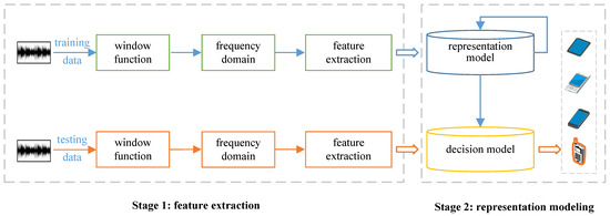
Figure 1.
Traditional recording device source identification consists of two main parts, which are feature expression and representation modeling.
2.1. Source Recording Device Identification Based on Feature Expression
Methods for source recording device identification based on feature expression can be classified into three types: the digital audio source information represent based on the frequency domain, the digital audio source information represent based on the statistical features, and the digital audio source information represent based on the bottleneck feature.
2.1.1. Digital Audio Source Information Representation Based on Frequency Domain
The representation of digital audio source information based on the frequency domain has been a significant focus in source recording device identification research. Buchholz et al. [17] introduced frequency domain features obtained through the short-time Fourier transform for source recording device identification, making a pioneering contribution to the field. Building upon this work, Kraetzer et al. [18] proposed the utilization of Mel Frequency Cepstral Coefficients (MFCC) features as machine fingerprints for identifying digital audio sources, thus advancing the study of source recording device identification. Hanilci et al. [19] extended these findings by employing MFCC as a channel feature for source recording device identification.
Subsequent studies conducted by Hanilci et al. [20,21] explored three additional cepstral features, namely Linear Frequency Cepstral Coefficients (LFCC), Bark Frequency Cepstral Coefficients (BFCC), and Linear Prediction Cepstral Coefficients (LPCC). Recognizing the characteristics of cepstral features, Zou et al. [22] proposed the use of Power-Normalized Cepstral Coefficients (PNCC) for analyzing source recording device identification. Researchers aimed to enhance the representation and generalization of these features, leading to the proposal of Labeled Spectral Features (LSF) by Panagakis et al. [23] and Sketches of Spectral Features (SSF) by Kotropoulos et al. [24,25]. To simplify the feature extraction process and reduce computational time, Luo et al. [6] represented channel features by calculating the baseband energy difference between adjacent frames, offering a streamlined approach to frequency domain feature extraction based on the short-time Fourier transform.
2.1.2. Digital Audio Source Information Representation Based on Statistical Features
Statistical features have also played a crucial role in the representation of digital audio source information for device identification. Kotropoulos et al. [26] and Zou et al. [27,28,29] utilized the MFCC features to train a Gaussian Mixture Model (GMM) as a Universal Background Model (UBM) [30]. They then employed the Maximum A Posteriori (MAP) algorithm to fine-tune the UBM model and obtain a relatively independent GMM. The representative Gaussian Supervectors (GSV) in the GMM were extracted as machine fingerprint features for identifying the source recording device.
To further improve the representation of GSV features, Li et al. [31,32] proposed a method for extracting deep GSV features. Instead of directly using MFCC features, they utilized the intermediate layer output of a Deep Neural Network (DNN) model trained on MFCC features as the data for training the GMM [33]. In an effort to investigate the impact of UBM on GSV features and enhance their representability, Jiang et al. [7] proposed mapping GSV features to a high-dimensional space. These advancements aimed to refine the statistical feature representation and improve the accuracy of source recording device identification.
2.1.3. Digital Audio Source Information Representation Based on Bottleneck Features
The utilization of deep neural networks in pattern identification has yielded significant advancements. Deep neural networks aim to extract bottleneck features inherent in the data through the network’s hidden layers, followed by decision output using a classifier. These bottleneck features are derived from the analysis and extraction of the inherent data characteristics [34,35].
Li et al. [31,32] proposed two types of bottleneck features. The first approach involves constructing a DNN using MFCC features and extracting the output of the network’s middle layer as a feature. The second approach entails training a deep self-encoder network with MFCC features and utilizing the output of the intermediate layer as the final output feature. By leveraging deep neural networks, these techniques enhance the representation of bottleneck features, contributing to the accurate identification of source recording devices.
2.2. Source Recording Device Identification Methods Based on Model Representation
In the field of source recording device identification, researchers have explored various models for representation modeling. These methods can be categorized into source recording device identification based on GMM, Support Vector Machine (SVM), other machine learning methods, and deep learning.
Currently, the majority of researchers employ support vector machines as the primary model for studying source recording device identification [36]. It is worth noting that while the use of support vector machines is prevalent, other models have also been investigated, showcasing the diverse approaches in this field.
2.2.1. Source Recording Device Identification Method Based on Gaussian Mixture Model
The GMM is a powerful tool for accurately representing the attribute characteristics of audio signals through a probability density model. In the context of source recording device identification, researchers have utilized GMMs as a method for modeling and analyzing digital audio sources. Several studies have employed the maximum likelihood function to train GMMs in source recording device identification.
Notably, Hanilci et al. [20], Eskidere et al. [35], Zou et al. [22], and Garcia-Romero et al. [34] incorporated the maximum likelihood function into their training procedures, enabling effective estimation of the model parameters. To further enhance the decision-making ability of GMMs, particularly in scenarios with limited data, Hanilçi et al. [20] introduced the concept of maximum mutual information to measure the performance of GMMs. By leveraging the capabilities of GMMs, researchers have made significant progress in accurately identifying and distinguishing different source recording devices.
2.2.2. Source Recording Device Identification Decision Model Based on Support Vector Machine
SVM has emerged as a popular model in machine learning for source recording device identification. SVM utilizes various kernel functions to map the input features into high-dimensional spaces, enabling the identification of device sources through the determination of suitable hyperplanes.
Notably, the Radial Basis Function (RBF) and Generalized Linear Discriminant Sequence (GLDS) kernels are commonly employed in SVM-based decision models [36]. Researchers widely rely on the LIBSVM toolkit [37] for conducting SVM experiments in the field of source recording device identification. This toolkit offers a convenient and practical implementation of SVM algorithms, allowing researchers to explore the capabilities of SVM in identifying and classifying digital audio sources. By leveraging SVM’s robust classification abilities, researchers have made significant advancements in accurately distinguishing source recording devices.
2.2.3. Source Recording Device Identification Decision Model Based on Other Machine Learning Methods
In addition to SVM, researchers have also investigated various traditional machine learning algorithms for making decisions in source recording device identification. These alternative methods offer different approaches to effectively classify and distinguish digital audio sources. Kraetzer et al. [18] introduced a Bayesian classifier that incorporates prior information and minimizes risk probability to serve as a decision model in source recording device identification. This approach leverages Bayesian principles to make informed decisions based on the available data and prior knowledge.
In their study, Kraetzer et al. [38] explored the use of linear logistic regression [39,40] and the C4.5 decision tree [41] as two distinct classifiers for feature fusion decisions. Linear logistic regression analyzes the relationship between the input features and the device sources, while the C4.5 decision tree algorithm constructs a tree-like model to classify and assign labels to the data based on specific feature thresholds. By employing these alternative machine learning methods, researchers expand the repertoire of decision models for source recording device identification, allowing for diverse approaches and potential improvements in accuracy and performance.
2.2.4. Digital Audio Source Decision Model Based on Deep Learning
Deep learning models have emerged as powerful tools, demonstrating exceptional performance across diverse domains. These models possess the ability to handle large datasets while exhibiting strong generalization and transferability capabilities. Consequently, researchers have directed their efforts toward developing deep learning-based decision models for representing digital audio sources. Several notable studies in this field are discussed below.
Qin et al. [42] constructed a Convolutional Neural Network (CNN) model [43,44] that utilized spectrograms of digital audio signals as input features. By leveraging the inherent structures in the spectrograms, the CNN model achieved promising results in identifying the source recording device. Baldini et al. [45,46] employed CNN to build a representation model after extracting relevant features from the audio signals. This approach improved the identification accuracy by effectively capturing discriminative patterns and representations.
To further enhance the representation capabilities of the CNN model, Zeng et al. [47] proposed a multi-feature parallel convolutional network combined with an attention mechanism. This architecture allowed the model to focus on important features while integrating multiple feature representations, leading to improved performance in source recording device identification tasks. Recognizing the sequential nature of audio data, Zeng et al. [14] suggested utilizing Long Short-Term Memory (LSTM) networks to construct an end-to-end identification model. By modeling the temporal dependencies in the audio data, the LSTM-based model achieved robust and accurate identification results.
The application of deep learning models in digital audio source identification shows promising potential for advancing the field, enabling more accurate and reliable identification of source recording devices.
3. Materials and Methods
3.1. Research Problem
The research problem addressed in this paper is source recording device identification for Audio Sustainable Security, which plays a crucial role in fields such as information security, digital forensics, copyright protection, and judicial fairness. Traditional methods have two main issues that need to be addressed. Firstly, they rely on manually designing features, where parameters such as frame length, and the use of first-order and second-order differences, greatly impact the recognition performance. However, the introduction of these manual parameters is time-consuming and results in poor generalization. Secondly, the back-end models and front-end feature representations in traditional methods are typically treated separately, lacking the ability to optimize the overall performance of feature representation and model decision-making at a global level.
The objective is to determine the identity of the recording device for a given test audio signal () by comparing it with an enrollment database (). The identification process is formulated as follows:
where represents a similarity function, denotes the parameters of the backend, and are the features of the enrollment and test devices, respectively, and D represents the number of enrollment devices. The problem can be categorized as either closed-set or open-set. In the closed-set scenario, will always correspond to one of the D registered devices, whereas in the open-set scenario, may not match any of the registered devices.
3.2. Proposed Method
In this section, we present our methodology for constructing an end-to-end transfer learning framework based on deep learning. Our approach integrates preprocessing, feature extraction, and representation modeling into a unified framework, allowing them to collectively participate in the network’s parameter optimization process. The flowchart of our method is depicted in Figure 2, providing an overview of the entire process.
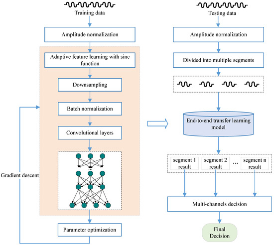
Figure 2.
Our proposed end-to-end transfer learning framework for source recording device identification integrates preprocessing, feature extraction, and representation modeling into a unified framework, allowing them to collectively participate in the network’s parameter optimization process.
3.2.1. Adaptive Feature Learning Method Based on the Sinc Function
In our methodology, we propose a deep neural network that consists of two main processes: forward propagation and backpropagation. During forward propagation, the network extracts the bottleneck feature vector from the input signal and passes it to the subsequent layers. In the backpropagation process, the neural network utilizes gradient optimization methods to adaptively learn the parameter values within the network. However, to enable differentiable forward calculations in the end-to-end network model, we employ the Sinc function to perform windowing, framing, and feature extraction operations on the input audio signal. The introduced Sinc function is a purely data-driven feature extraction method that does not require manually setting feature parameters. It can achieve efficient device features through optimized learning strategies. This also enables the construction of a DNN network that incorporates the Sinc-based features, and a multi-channel decision method is utilized to make decisions based on the feature vector.
In digital signal processing, when the original signal is convolved in the time domain with a finite impulse response filter, the convolution operation can be defined as follows:
Here, represents the original unprocessed audio signal, denotes the filter of length L, and represents the filtered signal. In traditional digital signal processing, each element of the filter is a pre-defined hyperparameter.
However, in the context of end-to-end processing, we aim to optimize the parameter selection and minimize the dependence on hyperparameters. To achieve this, we transform into a learnable convolution kernel of length L, where denotes the learnable parameter. Equation (2) can thus be transformed into:
By utilizing the Sinc function and the learnable convolution kernel, we enable the end-to-end network model to perform differentiable forward calculations, allowing for adaptive parameter optimization and reducing the reliance on hyperparameters.
In the field of digital signal processing, band-pass filters can be represented as the difference between two low-pass filters in the frequency domain. This allows us to express the convolution filter in Equation (4) as:
Here, and represent the low-frequency cut-off and high-frequency cut-off frequencies, respectively. These values are learned autonomously through the network. The function denotes a rectangular function in the amplitude frequency domain. After performing an inverse Fourier transform to the time domain, the function becomes:
An ideal band-pass filter is characterized by a perfectly flat pass-band and infinite attenuation in the stop-band [48]. However, achieving such an ideal filter would require an infinite number of filter elements, denoted as L. In practical applications, truncating the filter to a finite length inevitably leads to an approximation of the ideal filter, resulting in attenuation in the ripple pass-band and limited attenuation in the stop-band. To address this issue, a widely used solution is to apply a windowing function, denoted as , which eliminates the abrupt break at the end of the filter.
In practice, the function can only approximate an ideal band-pass filter, attenuating the ripple pass-band and providing limited attenuation in the stop-band. To mitigate the sudden truncation of the tail of the function , it is common to multiply it by the window function, resulting in Equation (6). The Hamming window, defined as Equation (7), is often used for this purpose:
Multiplying the truncated function by the window function yields the filter , which can be utilized to process the original input audio signal and extract the adaptive feature vector :
It is important to emphasize that all the parameters in the equations presented above are fully differentiable. This property enables the integration of the preprocessing and feature extraction processes into a deep neural network. By doing so, optimization techniques such as gradient descent can be employed to optimize the global network, automatically learning the optimal parameter values, including the cut-off frequency. Consequently, this approach mitigates problems associated with low generalization that can arise from manually setting parameters.
3.2.2. End-to-End Identification Method Based on Transfer Learning
The end-to-end identification method for digital audio sources aims to integrate feature extraction, representation modeling, and input-to-output timeliness. However, traditional deep neural network training faces challenges such as lengthy training times, high computational requirements, and the need for a large number of training samples. To address these issues, this paper proposes a transfer learning approach based on end-to-end neural networks, which can collaborate effectively with the Sinc function to achieve global optimization. Additionally, to enhance the identification accuracy of the transform neural network model, this study demonstrates that dividing the original input data into suitable small segments for joint decision-making can improve algorithm performance.
The proposed end-to-end identification method, based on transfer learning and multi-channel decision, consists of two stages: adaptive network model construction and automatic recognition. In the adaptive network model construction stage, the convolution window function is employed to extract adaptive feature vectors, denoted as , from the input signals . Subsequently, these feature vectors undergo preprocessing to achieve suitable dimensions, and their robustness is improved through down-sampling and regularization terms.
The above section provides an in-depth explanation of the adaptive feature learning process based on the convolution window function, highlighting that the feature vector extracted through adaptive feature learning effectively preserves the timing of the input signal. To ensure that the time sequence of the feature vector is not disrupted and that the representation of the feature vector is not compromised, a deep neural network (DNN) model is selected for constructing the neural network. Figure 3 illustrates the network structure.
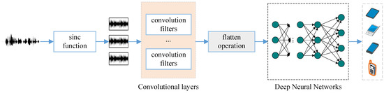
Figure 3.
Network structure.
Suppose that the actual output values obtained by the DNN are denoted as , and the expected outputs are represented by . Here, represents the training samples, where K denotes the total number of samples. The error E calculated using the cross-entropy function is defined as follows:
As both the computation of the feature learning process, represented by the cross-entropy function, and the convolution window function are differentiable, the Back Propagation (BP) algorithm is employed to train the network parameters layer by layer. The basic optimization process of the BP algorithm is summarized in Algorithm 1.
| Algorithm 1: Parameters optimization of end-to-end transfer learning framework for source recording device identification |
 |
3.2.3. Multi-Channels Decision Making
The above model is based on segment-level decisions. In this section, we propose a multi-channels decision approach to effectively enhance the robustness and accuracy of decision-making at the sample level. During the automatic identification stage, the input audio signal is first normalized and then divided into N short audio signals , where and l represent the length of the short sample. These short audio signals are sequentially input into the trained end-to-end migration model for decision-making, resulting in the output , where and . Here, N represents the number of categories, and the final decision is obtained using the joint judgment method described in (10). Specifically, the count of various decision results is denoted by , and the final result is determined as follows:
4. Experimental Results
In this section, we present a comprehensive experimental evaluation to demonstrate the effectiveness and advantages of our proposed method. We compare its performance with four baseline methods on two real datasets. Furthermore, we conduct an ablation study to analyze the individual components and key hyperparameters of our method. To determine the optimal parameter settings and structure, we perform experiments using our method.
The experimental evaluation serves two purposes. Firstly, it validates the effectiveness of each independent component of our framework by conducting an ablation study. This study follows the controlled variable method, allowing us to observe the impact of core modules and key hyperparameters on the overall performance. Through this analysis, we gain insights into the contribution of each component and fine-tune their settings for optimal results.
Secondly, we compare our method with four baseline methods on two real-world datasets. This comparison provides a comprehensive assessment of the performance of our approach. By evaluating it against the established four baselines, we can effectively measure its effectiveness and identify areas of improvement.
To ensure robustness and reliability, we conduct multiple experiments with different parameter configurations. By systematically varying the parameters and evaluating their impact, we obtain insights into the behavior and performance characteristics of our method. This rigorous experimentation allows us to draw accurate conclusions and make informed decisions regarding the parameter settings and overall structure of our approach.
4.1. Metric for Evaluation
In our experimental evaluation, we employ classification accuracy as the primary metric for evaluating the performance of the recording device identification system. Classification accuracy is a widely used metric in the field, providing an objective measure of performance and facilitating fair comparisons with the baseline methods. It allows for easy interpretation of the results and quantifies the proportion of correctly identified samples.
The identification accuracy of the audio sources is defined as follows:
where represents the total number of samples participating in the test, and represents the number of samples that were correctly identified by the system.
To compute the recognition results of the samples during the test, we utilize the final layer of our model, which incorporates a Softmax layer. The Softmax layer maps the output of each neuron in the penultimate fully connected layer to the interval , generating scores for each category in the multiclassification task. These scores are then used to calculate the probability of each sample belonging to a specific category, thereby obtaining the recognition results.
Furthermore, we conduct statistical significance tests to validate the observed performance differences between our method and the baseline methods. These tests provide a rigorous assessment of the significance of any observed variations in performance, ensuring the reliability and robustness of our comparative analysis.
By employing the classification accuracy metric and conducting statistical significance tests, we can confidently evaluate the performance of our method and establish its superiority over the baseline approaches. These evaluation techniques contribute to the objective assessment and reliable interpretation of the experimental results.
4.2. Baseline Methods
To evaluate the performance of the methods proposed in this paper, we compared them with several baseline methods. The baselines used in our comparison experiments are described below, providing a comprehensive benchmark for assessing the effectiveness of our proposed approaches. The details of each baseline method are as follows:
GMM-UBM [20]: This classical method utilizes Gaussian Mixture Models (GMM) for training and calculates probability scores for each category to perform identification. To reduce computational complexity, it employs a Universal Background Model (UBM) for training the GMM.
GSV-SVM [21]: This method leverages the Gaussian Supervector (GSV) representation as the frontend input to represent the audio sources. It then employs Support Vector Machines (SVM) as the backend identification model to classify the sources based on the GSV features.
MFCC-CNN [33]: This approach utilizes Mel Frequency Cepstral Coefficients (MFCC), a widely used spectral feature in audio recognition, as the input feature. It employs Convolutional Neural Networks (CNN) as the classification model to perform recording device identification.
GSV-CNN [14]: This method constructs a representative CNN model for recording device identification. The GSV features are regarded as the input representation for the CNN model.
By including these baseline methods, we establish a strong foundation for evaluating the performance of our proposed methods in comparison to well-established approaches in the field. The selected baselines cover both classical methods and representative deep learning methods, allowing us to assess the effectiveness and advantages of our proposed techniques.
4.3. Experimental Setting
A well-constructed dataset plays a crucial role in developing and evaluating algorithms in the field of source recording device identification. In this research domain, datasets can be categorized into two periods: the fixed-line period and the smart mobile device period. During the fixed-line period, datasets primarily consisted of recordings from fixed-line phones and microphones due to limitations imposed by social conditions. In the era of smart mobile devices, datasets shifted towards recordings from mobile phones, smartphones, and other mobile terminals to align with current technological trends and practical requirements.
Evaluation of datasets in the ASS domain of digital audio sources identification focuses on three primary criteria:
- Dataset size: A larger dataset includes a greater variety of device types and the audio data produced by each individual device becomes more extensive. This reduces the influence of data contingency and strengthens the reliability of experimental conclusions.
- Dataset diversity: Higher diversity in a dataset incorporates various factors such as equipment size, recording environment, and recording duration. This enables more detailed and profound investigations, leading to deeper insights.
- Practical relevance: The dataset should align with practical needs while satisfying the aforementioned criteria. Considering the requirements of large-scale network models based on deep neural networks, which necessitate large and diverse datasets, we developed the CCNU_Mobile dataset by taking into account the experimental context and leveraging existing research resources. The details of the equipment used in this dataset are presented in Table 1.
 Table 1. The brands, numbers, and models involved in CCNU_Mobile dataset.
To encompass a broader range of device characteristics and enrich sample diversity, the CCNU_Mobile dataset includes audio data recorded on 45 different devices from 8 distinct brands, including a small number of iPads. Additionally, devices of the same type were selected for recording to facilitate in-depth exploration of device fingerprint information generated by different types and models of equipment. For example, devices A1 to A4 belong to the iPhone 6 series, representing four distinct devices. To minimize interference from external devices and ensure consistent content across recordings, we utilized the original and unaltered TIMIT dataset [49] (without transcription by other devices) as the source material. However, since the TIMIT dataset consists of small audio segments, it was impractical to directly record from it. Therefore, we compiled all the training data from the TIMIT dataset, merging them into a single, continuous corpus with a duration of approximately 110 min. To ensure recording quality, the same laptop was employed for playback and recording in batches within a dedicated and acoustically controlled recording studio. The recorded audio data had a sampling rate of 32 kHz and a quantization rate of 16 bits. Next, using an active audio detection method, we removed silent segments from the beginning and end of the recorded long audio data. Finally, to facilitate subsequent analysis, we divided the long audio data into 642 small-sample segments based on the original order of the samples during the merging process, with each segment having a duration of approximately 10 s.
4.4. Comparing with State-of-the-Art Methods
To evaluate the effectiveness of our proposed method, we conducted a comparative analysis with state-of-the-art methods in the field of source recording device identification.
In order to ensure the validity of the dataset and account for the challenges associated with large-scale experimental analyses of certain basic methods, we performed a controlled experiment using both the MOBIPHONE dataset (21 classes) and our CCNU_Mobile dataset. The experimental methodology and parameter settings are outlined as follows:
We utilized the TIMIT dataset as a reference dataset, from which we extracted 39-dimensional Mel-frequency cepstral coefficient (MFCC) features. These features included first-order difference scores, second-order difference scores, and F0 coefficients. Subsequently, we trained a Gaussian Mixture Model - Universal Background Model (GMM_UBM) containing 64 Gaussian components using the extracted MFCC features. The same 39-dimensional MFCC features extracted from the training dataset were then input into the GMM_UBM model to extract Gaussian Supervector (GSV) features. This process allowed us to compare the performance of our proposed method against the selected state-of-the-art methods.
The experimental results obtained using the aforementioned methodology and parameter design are presented in Table 2, which showcases the performance of four basic methods alongside our proposed method.
Table 2.
Our proposed end-to-end source recording device identification is compared with four state-of-the-art methods. Bold indicates the best predicted performance, and underline indicates the second best predicted performance.
Table 2 provides a comprehensive comparison of the performance of different methods across the MOBIPHONE and CCNU_Mobile datasets. The results demonstrate the superiority of our proposed method, achieving significantly higher accuracy rates compared to the state-of-the-art techniques. Specifically, as shown in Figure 4 and Figure 5, our method achieved an accuracy rate of 92.3% on the MOBIPHONE dataset and 97.7% on the CCNU_Mobile dataset, outperforming the other methods. These outcomes validate the effectiveness and potential of our approach in accurately identifying the source recording device.
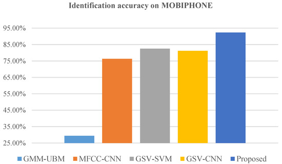
Figure 4.
Our proposed method compared to four state-of-the-art methods on MOBIPHONE dataset. The proposed method is better than the other four baseline methods, with an absolute 9.8% improvement in identification accuracy.
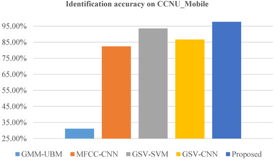
Figure 5.
Our proposed method compared to four state-of-the-art methods on the MOBIPHONE dataset. The proposed method is better than the other four baseline methods, with an absolute 4.1% improvement in identification accuracy.
4.5. The Effectiveness of the Transfer Learning Framework
In this section, we evaluate the effectiveness of our proposed transfer learning framework.
Initially, we selected 100 sample audio data from each device in the CCNU_Mobile dataset to train the end-to-end base model. The model training stage involved the use of 80 Sinc window functions with a length of 251 (the initial cutoff frequency of the window function was based on the Mel frequency) for convolution to extract features.
Subsequently, 2 successive convolutional layers were constructed, utilizing 60 convolution kernels of length 5 in the convolutional layer to extract bottleneck features. Finally, the normalized feature data was fed into a 3-layer DNN network with 2048 nodes in each layer.
During the transfer training stage, we intercepted six short audio segments from each category of audio data in the Uncontrolled-Conditions dataset, maintaining a sample duration of 18 s. To test the performance of the end-to-end method on small-sample datasets, one sample was used for training, and five samples were used for testing. We conducted three experimental groups to examine the performance of different transfer learning methods.
In the first experimental group, no model was transferred, and the samples from the Uncontrolled-Conditions dataset were used for training and testing, as shown in Figure 6. In the second experimental group, as shown in Figure 7, we transferred and froze the parameters of the adaptive feature learning layer from the base model, while randomly initializing and training the DNN network layer. In the third experimental group, we transferred all parameters of the base network except for the last layer as initial values and trained the network model, as shown in Figure 8. To assess the timeliness of the 3 methods, we conducted tests on the test data every 1600 epochs. Table 3 displays the first four test results for the three training methods, with “single” denoting single-channel decisions, and “multi” denoting multi-channel decisions.
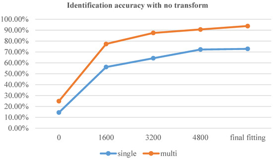
Figure 6.
Identification accuracy with no transform operation.
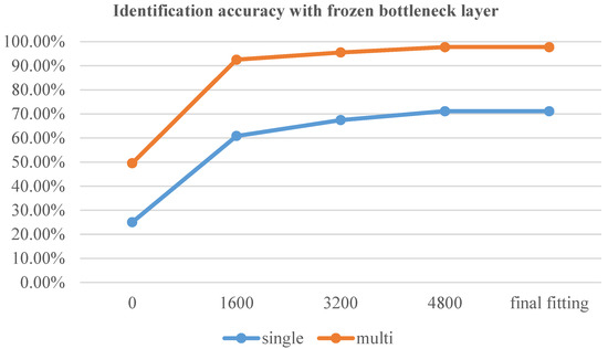
Figure 7.
Identification accuracy with frozen bottleneck layer.
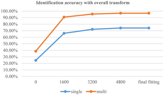
Figure 8.
Identification accuracy with overall transform.
Table 3.
Ablation experiments based on different combinations of parameters.
The experiment results, presented in Table 3, provide valuable insights into the effectiveness of the transfer learning framework and its impact on source recording device identification.
Through a comparative analysis of the table, we can draw the following three conclusions:
- The multi-channel decision end-to-end identification method based on the Sinc function demonstrates significant effectiveness in the research field of source recording device identification. This finding highlights that the end-to-end identification method, which combines deep neural network fusion, not only enhances the operability of end-to-end recognition but also improves the overall identification accuracy.
- The utilization of multi-channel decisions significantly enhances the identification performance of digital audio sources. This observation suggests that although some feature data may be lost during the audio signal segmentation process, the comprehensive decision-making ability can be improved through reasonable segmentation techniques.
- Comparative analysis with the non-transfer method reveals that the end-to-end identification method based on transfer learning requires fewer training iterations to achieve the same level of identification accuracy. This finding indicates that the transfer learning approach offers stronger timeliness, enabling faster resolution of practical problems. Consequently, it is highly advantageous for the application of end-to-end source recording device identification.
These conclusions validate the effectiveness and practicality of our proposed transfer learning framework in the domain of source recording device identification. By leveraging transfer learning, we can achieve improved identification accuracy with reduced training requirements, making the approach highly applicable and efficient.
It is worth noting that these conclusions are based on the experimental results obtained from the three training methods. The accuracy percentages presented in Table 3 reflect the performance at different epochs during the training process.
5. Discussion
The field of digital audio source identification has seen significant advancements in recent years, particularly in the development of end-to-end identification methods. However, there are several limitations and challenges that need to be addressed in order to enhance the performance and practicality of these methods. In this section, we will discuss the motivations behind this research and highlight the gaps in existing approaches.
Firstly, it is important to note that most current end-to-end identification methods for digital audio sources involve a sequential process of feature extraction and representation modeling. While this approach has yielded promising results, it lacks integration and can lead to suboptimal performance. The separation of feature extraction and representation modeling can result in a loss of important information and a lack of coherence in the overall model. This limitation is illustrated in Figure 1, where the disjointed nature of the step-by-step approach is evident. Therefore, there is a need to explore alternative methods that can overcome this limitation and achieve better integration between feature extraction and representation modeling.
Secondly, feature extraction is a critical step in the identification process as it directly impacts the final decision. Traditional methods heavily rely on human domain knowledge to design and extract relevant features from the audio data. This manual feature engineering process can be time-consuming and challenging, especially as the volume of data increases. Furthermore, it requires significant expertise and prior knowledge to determine the most informative features for accurate identification. As a result, the stability and generalization of traditional end-to-end identification algorithms are compromised. To address these limitations, it is necessary to investigate new approaches that can automate the feature extraction process and allow the model to learn and extract discriminative features directly from the raw data.
Thirdly, the parameterization of the identification models poses another challenge. In traditional approaches, various parameters need to be manually set and tuned, which can be a tedious and subjective process. The difficulty lies in finding the optimal parameter configuration that yields the best performance. As the number of parameters and the complexity of the models increase, the search space for finding the optimal configuration becomes exponentially larger, making it impractical to exhaustively explore all possibilities. Consequently, traditional methods often settle for suboptimal parameter settings, hindering the overall performance and generalization of the identification models. Therefore, it is crucial to investigate approaches that can alleviate this burden by allowing the model to autonomously learn and optimize the parameters.
Deep neural networks offer a promising solution to address the aforementioned limitations and challenges. These networks have the capability to integrate feature extraction and representation modeling into a unified process, enabling end-to-end learning. By leveraging the power of deep learning, the network can automatically learn and extract relevant features from the raw audio data without the need for manual feature engineering. This eliminates the reliance on human prior knowledge and enhances the adaptability and generalization of the identification models. Furthermore, the parameter optimization process in deep neural networks can be performed collectively, allowing the network to learn the optimal parameters that maximize the global objective function. This reduces the subjective manual parameter tuning and enhances the stability and performance of the identification models.
In summary, this study aims to address the limitations of traditional end-to-end identification methods by proposing a deep neural network framework that integrates preprocessing, feature extraction, and representation modeling. By synchronously participating in the network’s parameter optimization process, we expect to enhance stability, improve identification performance, and overcome the challenges posed by manual feature engineering and parameter tuning. Additionally, the exploration of end-to-end transfer learning models offers potential solutions to the issues associated with small sample datasets and time-consuming model training. By leveraging transfer learning, we aim to improve the efficiency, generalization, and robustness in digital audio source identification.
Our experimental verification demonstrates that the proposed end-to-end transfer learning model achieves timely and accurate results, even with small sample sizes. Moreover, it avoids the need for retraining the model with a large number of samples due to incremental expression. Our experiments showcase the superiority of our method, achieving an impressive 97.7% accuracy when identifying 141 devices. This outperforms four state-of-the-art methods, demonstrating an absolute accuracy improvement of 4.1%. These results provide strong evidence of the effectiveness and advantages of our proposed approach.
This research contributes significantly to the field of audio source identification by addressing key limitations and challenges in existing methods. By integrating preprocessing, feature extraction, and representation modeling in a unified framework, we enhance the overall performance and practicality of end-to-end identification methods. The automation of feature extraction and parameter optimization processes eliminates the need for manual feature engineering and subjective parameter tuning, improving the stability, adaptability, and generalization of the identification models. Additionally, the exploration of end-to-end transfer learning models addresses the issues related to small sample sizes and time-consuming model training, further enhancing efficiency, generalization, and robustness in audio source identification.
The insights gained from this study pave the way for future research in audio source identification and related applications. Further investigation can be conducted to explore advanced deep learning architectures, such as attention mechanisms or graph neural networks, to further enhance the performance of identification models. Additionally, the incorporation of other modalities, such as text or image data, can expand the scope and applicability of audio source identification in multimedia analysis. Furthermore, the deployment of the proposed method in real-world scenarios and the evaluation of its performance under various challenging conditions can provide valuable insights for practical applications.
In conclusion, this research addresses the limitations of traditional end-to-end identification methods and proposes a deep neural network framework that integrates preprocessing, feature extraction, and representation modeling. The experimental results demonstrate the superiority of our method over state-of-the-art approaches, achieving high accuracy and outperforming existing baselines. The findings of this study contribute to the advancement of audio source identification techniques and provide valuable insights for future research in the field.
6. Conclusions
The proposed end-to-end identification method for source recording device identification has been thoroughly investigated in this paper. Addressing the limitations of traditional step-by-step optimization approaches, we introduced the Sinc window function method to preprocess the raw data and extract feature information. By combining this method with a neural network representation model, we developed a comprehensive end-to-end model for source recording device identification, enabling participation in the global optimization process. The theoretical and experimental demonstrations in Section 3 and Section 4 support the efficacy of our approach.
While our work has yielded promising results in the realm of end-to-end identification of digital audio sources, there remains ample room for further exploration and improvement. In our future endeavors, we plan to delve deeper into the selection of representation models, aiming to identify more suitable network models and compare their performance with our proposed method. Additionally, we will conduct in-depth research on feature extraction window functions, optimizing their construction methods to enhance their feature extraction capabilities. Moreover, we will focus on advancing the segmentation of audio signals, aiming to establish a robust basis and segmentation method for audio segmentation within our framework. In future research, we will conduct additional experiments to further validate the effectiveness of our method in the fields of information security, digital forensics, copyright protection, and others.
Lastly, we recognize the importance of computational cost and performance improvement in end-to-end network models. Consequently, we intend to explore methods to reduce computational costs and enhance the overall performance of the network model. These investigations will contribute to creating more efficient and effective end-to-end source recording device identification systems.
Author Contributions
Conceptualization, Z.W. and J.Z.; methodology, Z.W.; software, Z.W. and J.Z.; validation, Z.W., J.Z., G.Z., D.O. and H.G.; formal analysis, Z.W.; investigation, Z.W., J.Z., G.Z., D.O. and H.G.; resources, Z.W.; data curation, Z.W.; writing—original draft preparation, Z.W. and J.Z.; writing—review and editing, Z.W. and J.Z.; visualization, Z.W. and J.Z.; supervision, Z.W.; project administration, Z.W.; funding acquisition, Z.W. All authors have read and agreed to the published version of the manuscript.
Funding
The research work in this paper was supported by the National Natural Science Foundation of China (No. 62177022, 61901165, 61501199), AI and Faculty Empowerment Pilot Project (No. CCNUAI&FE2022-03-01), Collaborative Innovation Center for Informatization and Balanced Development of K-12 Education by MOE and Hubei Province (No. xtzd2021-005), and Natural Science Foundation of Hubei Province (No. 2022CFA007).
Institutional Review Board Statement
Not applicable.
Informed Consent Statement
Not applicable.
Data Availability Statement
Data will be made available on reasonable request.
Conflicts of Interest
The authors declare no conflict of interest.
Abbreviations
The following abbreviations are used in this manuscript:
| ASS | Audio Sustainable Security |
| BFCC | Bark Frequency Cepstral Coefficients |
| CNN | Convolutional Neural Network |
| DNN | Deep Neural Network |
| GLDS | Generalized Linear Discriminant Sequence |
| GMM | Gaussian Mixture Model |
| GSV | Gaussian Supervectors |
| LFCC | Linear Frequency Cepstral Coefficients |
| LPCC | Linear Prediction Cepstral Coefficients |
| LSF | Labeled Spectral Features |
| LSTM | Long Short-Term Memory |
| MAP | Maximum A Posteriori |
| MFCC | Mel Frequency Cepstral Coefficients |
| PNCC | Power-Normalized Cepstral Coefficients |
| RBF | Radial Basis Function |
| SSF | Sketches of Spectral Features |
| SVM | Support Vector Machine |
References
- Ustubioglu, B.; Tahaoglu, G.; Ulutas, G. Detection of Audio Copy-Move-Forgery with Novel Feature Matching on Mel Spectrogram. Expert Syst. Appl. 2023, 213, 118963. [Google Scholar] [CrossRef]
- Zeng, C.; Kong, S.; Wang, Z.; Li, K.; Zhao, Y. Digital Audio Tampering Detection Based on Deep Temporal–Spatial Features of Electrical Network Frequency. Information 2023, 14, 253. [Google Scholar] [CrossRef]
- Shen, X.; Shao, X.; Ge, Q.; Liu, L. RARS: Recognition of Audio Recording Source Based on Residual Neural Network. IEEE/ACM Trans. Audio Speech Lang. Process. 2021, 29, 575–584. [Google Scholar] [CrossRef]
- Wang, P.; Gao, H.; Guo, X.; Yuan, Z.; Nian, J. Improving the Security of Audio CAPTCHAs with Adversarial Examples. IEEE Trans. Dependable Secur. Comput. 2023, 32, 1–18. [Google Scholar] [CrossRef]
- Zeng, C.; Feng, S.; Zhu, D.; Wang, Z. Source Acquisition Device Identification from Recorded Audio Based on Spatiotemporal Representation Learning with Multi-Attention Mechanisms. Entropy 2023, 25, 626. [Google Scholar] [CrossRef]
- Luo, D.; Korus, P.; Huang, J. Band Energy Difference for Source Attribution in Audio Forensics. IEEE Trans. Inf. Forensics Secur. 2018, 13, 2179–2189. [Google Scholar] [CrossRef]
- Jiang, Y.; Leung, F.H.F. Source Microphone Recognition Aided by a Kernel-Based Projection Method. IEEE Trans. Inf. Forensics Secur. 2019, 14, 2875–2886. [Google Scholar] [CrossRef]
- Park, N.I.; Lim, S.H.; Byun, J.S.; Kim, J.H.; Lee, J.W.; Chun, C.; Kim, Y.; Jeon, O.Y. Forensic Authentication Method for Audio Recordings Generated by Voice Recorder Application on Samsung Galaxy Watch4 Series. J. Forensic Sci. 2023, 68, 139–153. [Google Scholar] [CrossRef]
- Lin, X.; Zhu, J.; Chen, D. Subband Aware CNN for Cell-Phone Recognition. IEEE Signal Process. Lett. 2020, 27, 605–609. [Google Scholar] [CrossRef]
- Hua, G.; Wang, Q.; Ye, D.; Zhang, H.; Wang, G.; Xia, S. Factors Affecting Forensic Electric Network Frequency Matching—A Comprehensive Study. Digit. Commun. Netw. 2023, 9. [Google Scholar] [CrossRef]
- Zeng, C.; Yang, Y.; Wang, Z.; Kong, S.; Feng, S. Audio Tampering Forensics Based on Representation Learning of ENF Phase Sequence. Int. J. Digit. Crime Forensics 2022, 14, 1–19. [Google Scholar] [CrossRef]
- Verma, V.; Khanna, N. Speaker-Independent Source Cell-Phone Identification for Re-Compressed and Noisy Audio Recordings. Multimed. Tools Appl. 2021, 80, 23581–23603. [Google Scholar] [CrossRef]
- Wang, Z.; Yang, Y.; Zeng, C.; Kong, S.; Feng, S.; Zhao, N. Shallow and Deep Feature Fusion for Digital Audio Tampering Detection. EURASIP J. Adv. Signal Process. 2022, 2022, 69. [Google Scholar] [CrossRef]
- Zeng, C.; Zhu, D.; Wang, Z.; Wu, M.; Xiong, W.; Zhao, N. Spatial and Temporal Learning Representation for End-to-End Recording Device Identification. EURASIP J. Adv. Signal Process. 2021, 2021, 41. [Google Scholar] [CrossRef]
- Baldini, G.; Amerini, I. An Evaluation of Entropy Measures for Microphone Identification. Entropy 2020, 22, 1235. [Google Scholar] [CrossRef]
- Jin, C.; Wang, R.; Yan, D. Source Smartphone Identification by Exploiting Encoding Characteristics of Recorded Speech. Digit. Investig. 2019, 29, 129–146. [Google Scholar] [CrossRef]
- Buchholz, R.; Kraetzer, C.; Dittmann, J. Microphone Classification Using Fourier Coefficients. In Proceedings of the Information Hiding; Katzenbeisser, S., Sadeghi, A.R., Eds.; Lecture Notes in Computer Science; Springer: Berlin/Heidelberg, Germany, 2009; pp. 235–246. [Google Scholar] [CrossRef]
- Kraetzer, C.; Oermann, A.; Dittmann, J.; Lang, A. Digital Audio Forensics: A First Practical Evaluation on Microphone and Environment Classification. In Proceedings of the 9th Workshop on Multimedia & Security, MM&Sec ’07, Dallas, TX, USA, 20–21 September 2007; pp. 63–74. [Google Scholar] [CrossRef]
- Hanilci, C.; Ertas, F.; Ertas, T.; Eskidere, Ö. Recognition of Brand and Models of Cell-Phones From Recorded Speech Signals. IEEE Trans. Inf. Forensics Secur. 2012, 7, 625–634. [Google Scholar] [CrossRef]
- Hanilçi, C.; Ertas, F. Optimizing Acoustic Features for Source Cell-Phone Recognition Using Speech Signals. In Proceedings of the First ACM Workshop on Information Hiding and Multimedia Security, IH&MMSec ’13, Montpellier, France, 17–19 June 2013; pp. 141–148. [Google Scholar] [CrossRef]
- Hanilçi, C.; Kinnunen, T. Source Cell-Phone Recognition from Recorded Speech Using Non-Speech Segments. Digit. Signal Process. 2014, 35, 75–85. [Google Scholar] [CrossRef]
- Zou, L.; Yang, J.; Huang, T. Automatic Cell Phone Recognition from Speech Recordings. In Proceedings of the 2014 IEEE China Summit & International Conference on Signal and Information Processing (ChinaSIP), Xi’an, China, 9–13 July 2014; pp. 621–625. [Google Scholar] [CrossRef]
- Panagakis, Y.; Kotropoulos, C. Telephone Handset Identification by Feature Selection and Sparse Representations. In Proceedings of the 2012 IEEE International Workshop on Information Forensics and Security (WIFS), Tenerife, Spain, 2–5 December 2012; pp. 73–78. [Google Scholar] [CrossRef]
- Kotropoulos, C. Telephone Handset Identification Using Sparse Representations of Spectral Feature Sketches. In Proceedings of the 2013 International Workshop on Biometrics and Forensics (IWBF), Lisbon, Portugal, 4–5 April 2013; pp. 1–4. [Google Scholar] [CrossRef]
- Kotropoulos, C.L. Source Phone Identification Using Sketches of Features. IET Biom. 2014, 3, 75–83. [Google Scholar] [CrossRef]
- Kotropoulos, C.; Samaras, S. Mobile Phone Identification Using Recorded Speech Signals. In Proceedings of the 2014 19th International Conference on Digital Signal Processing, Hong Kong, China, 20–23 August 2014; pp. 586–591. [Google Scholar] [CrossRef]
- Zou, L.; He, Q.; Wu, J. Source Cell Phone Verification from Speech Recordings Using Sparse Representation. Digit. Signal Process. 2017, 62, 125–136. [Google Scholar] [CrossRef]
- Zou, L.; He, Q.; Feng, X. Cell Phone Verification from Speech Recordings Using Sparse Representation. In Proceedings of the 2015 IEEE International Conference on Acoustics, Speech and Signal Processing (ICASSP), South Brisbane, Australia, 19–24 April 2015; pp. 1787–1791. [Google Scholar] [CrossRef]
- Zou, L.; He, Q.; Yang, J.; Li, Y. Source Cell Phone Matching from Speech Recordings by Sparse Representation and KISS Metric. In Proceedings of the 2016 IEEE International Conference on Acoustics, Speech and Signal Processing (ICASSP), Shanghai, China, 20–25 March 2016; pp. 2079–2083. [Google Scholar] [CrossRef]
- Reynolds, D.A.; Quatieri, T.F.; Dunn, R.B. Speaker Verification Using Adapted Gaussian Mixture Models. Digit. Signal Process. 2000, 10, 19–41. [Google Scholar] [CrossRef]
- Li, Y.; Zhang, X.; Li, X.; Feng, X.; Yang, J.; Chen, A.; He, Q. Mobile Phone Clustering from Acquired Speech Recordings Using Deep Gaussian Supervector and Spectral Clustering. In Proceedings of the 2017 IEEE International Conference on Acoustics, Speech and Signal Processing (ICASSP), New Orleans, LA, USA, 5–9 March 2017; pp. 2137–2141. [Google Scholar] [CrossRef]
- Li, Y.; Zhang, X.; Li, X.; Zhang, Y.; Yang, J.; He, Q. Mobile Phone Clustering From Speech Recordings Using Deep Representation and Spectral Clustering. IEEE Trans. Inf. Forensics Secur. 2018, 13, 965–977. [Google Scholar] [CrossRef]
- Hinton, G.; Deng, L.; Yu, D.; Dahl, G.E.; Mohamed, A.r.; Jaitly, N.; Senior, A.; Vanhoucke, V.; Nguyen, P.; Sainath, T.N.; et al. Deep Neural Networks for Acoustic Modeling in Speech Recognition: The Shared Views of Four Research Groups. IEEE Signal Process. Mag. 2012, 29, 82–97. [Google Scholar] [CrossRef]
- Garcia-Romero, D.; Espy-Wilson, C.Y. Automatic Acquisition Device Identification from Speech Recordings. In Proceedings of the 2010 IEEE International Conference on Acoustics, Speech and Signal Processing, Dallas, TX, USA, 14–19 March 2010; pp. 1806–1809. [Google Scholar] [CrossRef]
- Eskidere, Ö.; Karatutlu, A. Source Microphone Identification Using Multitaper MFCC Features. In Proceedings of the 2015 9th International Conference on Electrical and Electronics Engineering (ELECO), Bursa, Turkey, 26–28 November 2015; pp. 227–231. [Google Scholar] [CrossRef]
- Campbell, W.M. Generalized Linear Discriminant Sequence Kernels for Speaker Recognition. In Proceedings of the 2002 IEEE International Conference on Acoustics, Speech, and Signal Processing, Orlando, FL, USA, 13–17 May 2002; Volume 1, pp. I–161–I–164. [Google Scholar] [CrossRef]
- Chang, C.C.; Lin, C.J. LIBSVM: A Library for Support Vector Machines. ACM Trans. Intell. Syst. Technol. 2011, 2, 27. [Google Scholar] [CrossRef]
- Kraetzer, C.; Schott, M.; Dittmann, J. Unweighted Fusion in Microphone Forensics Using a Decision Tree and Linear Logistic Regression Models. In Proceedings of the 11th ACM Workshop on Multimedia and Security, MM&Sec ’09, Princeton, NJ, USA, 7–8 September 2009; pp. 49–56. [Google Scholar] [CrossRef]
- Austin, P.C. A Comparison of Regression Trees, Logistic Regression, Generalized Additive Models, and Multivariate Adaptive Regression Splines for Predicting AMI Mortality. Stat. Med. 2007, 26, 2937–2957. [Google Scholar] [CrossRef]
- Birkenes, Ø.; Matsui, T.; Tanabe, K.; Siniscalchi, S.M.; Myrvoll, T.A.; Johnsen, M.H. Penalized Logistic Regression with HMM Log-Likelihood Regressors for Speech Recognition. IEEE Trans. Audio Speech Lang. Process. 2010, 18, 1440–1454. [Google Scholar] [CrossRef]
- Quinlan, J.R. C4.5: Programs for Machine Learning; Elsevier: Amsterdam, The Netherlands, 2014. [Google Scholar]
- Qin, T.; Wang, R.; Yan, D.; Lin, L. Source Cell-Phone Identification in the Presence of Additive Noise from CQT Domain. Information 2018, 9, 205. [Google Scholar] [CrossRef]
- LeCun, Y.; Boser, B.; Denker, J.S.; Henderson, D.; Howard, R.E.; Hubbard, W.; Jackel, L.D. Backpropagation Applied to Handwritten Zip Code Recognition. Neural Comput. 1989, 1, 541–551. [Google Scholar] [CrossRef]
- Lecun, Y.; Bottou, L.; Bengio, Y.; Haffner, P. Gradient-Based Learning Applied to Document Recognition. Proc. IEEE 1998, 86, 2278–2324. [Google Scholar] [CrossRef]
- Garcia-Romero, D.; Espy-Wilson, C. Speech Forensics: Automatic Acquisition Device Identification. J. Acoust. Soc. Am. 2010, 127, 2044. [Google Scholar] [CrossRef]
- Baldini, G.; Amerini, I.; Gentile, C. Microphone Identification Using Convolutional Neural Networks. IEEE Sens. Lett. 2019, 3, 1–4. [Google Scholar] [CrossRef]
- Zeng, C.; Zhu, D.; Wang, Z.; Wang, Z.; Zhao, N.; He, L. An End-to-End Deep Source Recording Device Identification System for Web Media Forensics. Int. J. Web Inf. Syst. 2020, 16, 413–425. [Google Scholar] [CrossRef]
- Ravanelli, M.; Bengio, Y. Interpretable Convolutional Filters with SincNet. arXiv 2019, arXiv:1811.09725. [Google Scholar] [CrossRef]
- Garofolo, J.S.; Lamel, L.F.; Fisher, W.M.; Fiscus, J.G.; Pallett, D.S. Getting Started with the DARPA TIMIT CD-ROM: An Acoustic Phonetic Continuous Speech Database; National Institute of Standards and Technology (NIST): Gaithersburgh, MD, USA, 1988; Volume 107, p. 16. [Google Scholar]
Disclaimer/Publisher’s Note: The statements, opinions and data contained in all publications are solely those of the individual author(s) and contributor(s) and not of MDPI and/or the editor(s). MDPI and/or the editor(s) disclaim responsibility for any injury to people or property resulting from any ideas, methods, instructions or products referred to in the content. |
© 2023 by the authors. Licensee MDPI, Basel, Switzerland. This article is an open access article distributed under the terms and conditions of the Creative Commons Attribution (CC BY) license (https://creativecommons.org/licenses/by/4.0/).