

Towards a More Sustainable and Less Invasive Approach for the Investigation of Modern and Contemporary Paintings

 , ,
, ,  ,
,
Abstract
:1. Introduction
1.1. Sustainable Approaches—The Answer to the Need for a More Effective and Less Invasive Analysis of Modern and Contemporary Paintings
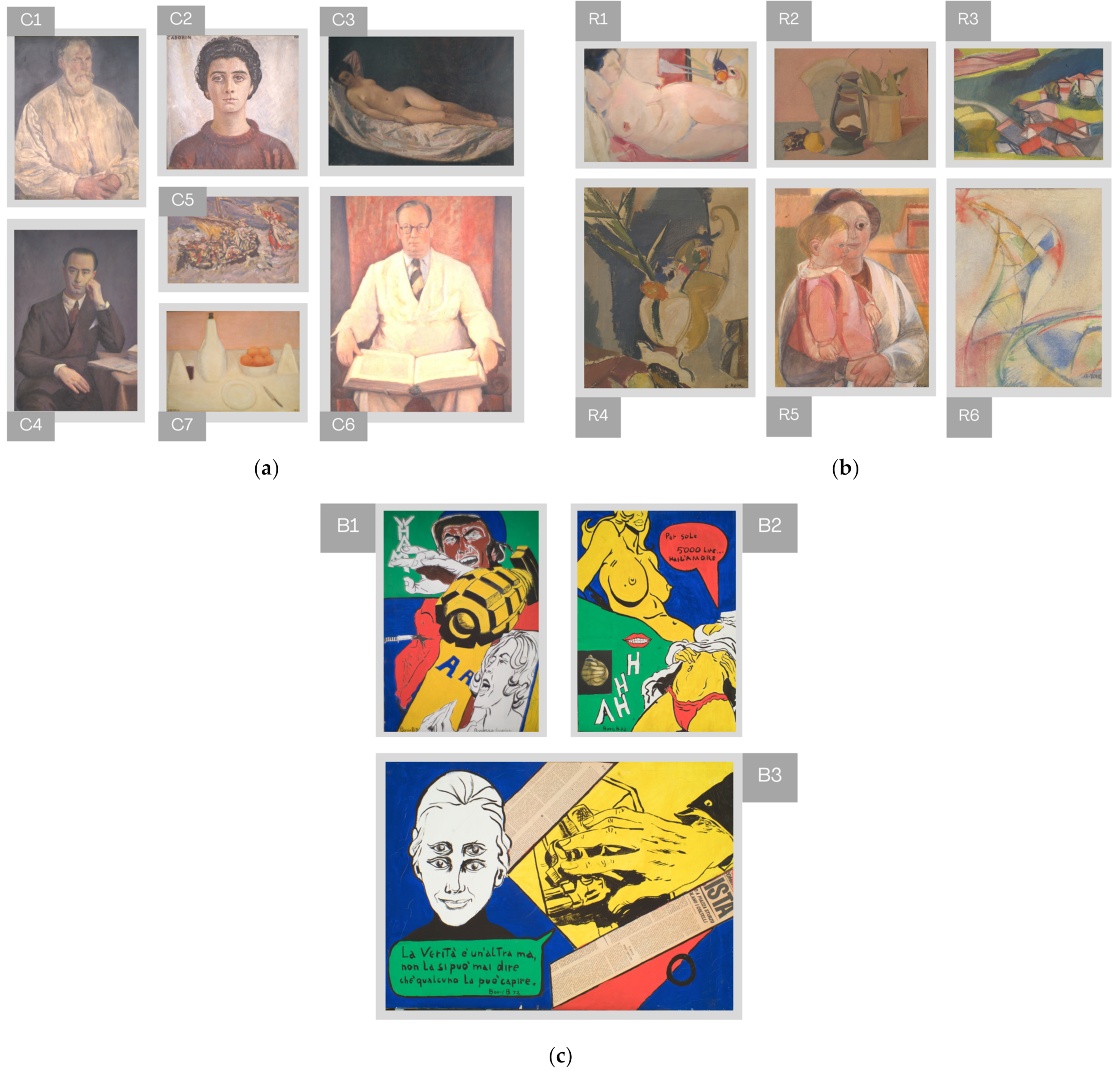
1.2. The Paintings Included in this Study
1.3. The Aim of this Research
2. Materials and Methods
2.1. The Non-Invasive Analytical Techniques Used for the Identification of the Painting Materials of Boris Brollo
2.1.1. Raman Spectroscopy
2.1.2. External Reflection FTIR Spectroscopy (ER–FTIR)
2.2. The Proposed Computational Approach for the Preliminary Identification of Pigment Mixtures
2.2.1. Camera, Color Target, and Spectrocolorimetry
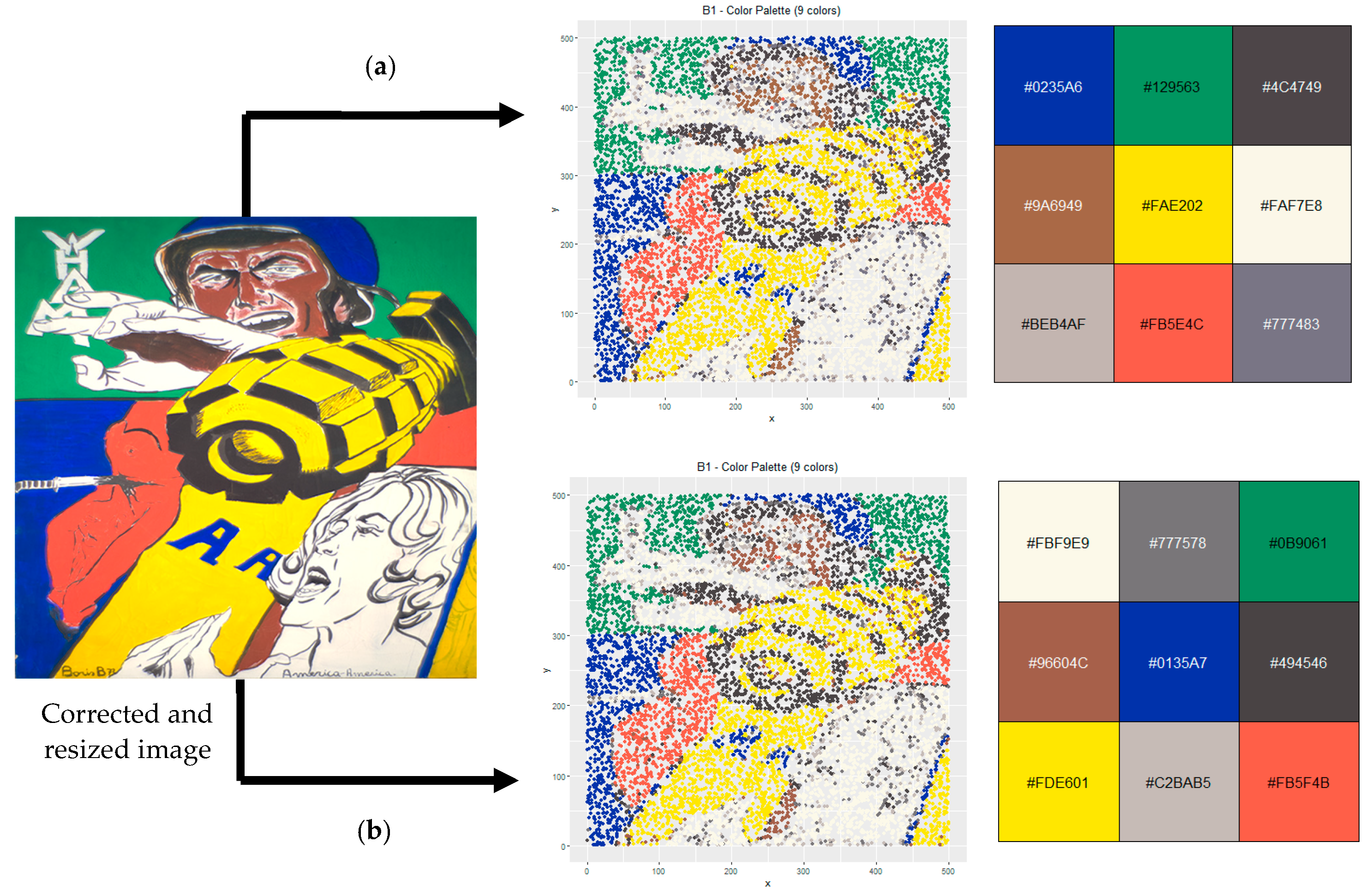
2.2.2. Color Correction of the Images
2.2.3. Image Resizing and Data Frame Arrangement
2.2.4. Image Sampling and the Selection of the Number of Clusters
2.2.5. 3D and 2D Color Histograms (sRGB Color Space)
2.2.6. K-Means and Fuzzy C-Means Clustering for the Extraction of the Color Palettes
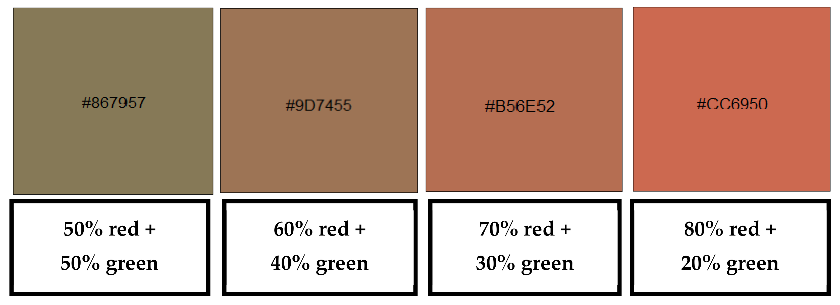
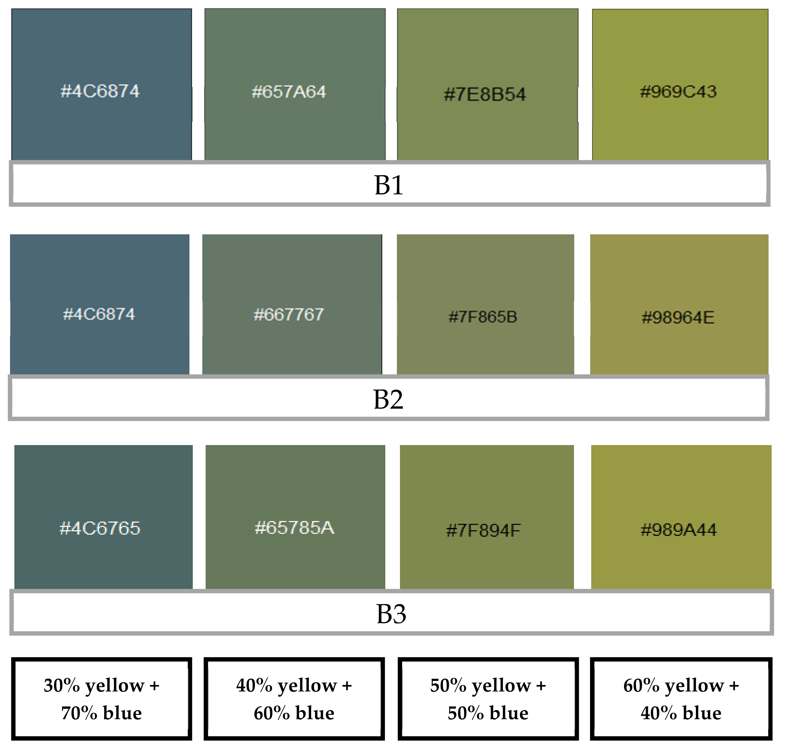
2.2.7. Simulation of Mixtures of Pigments
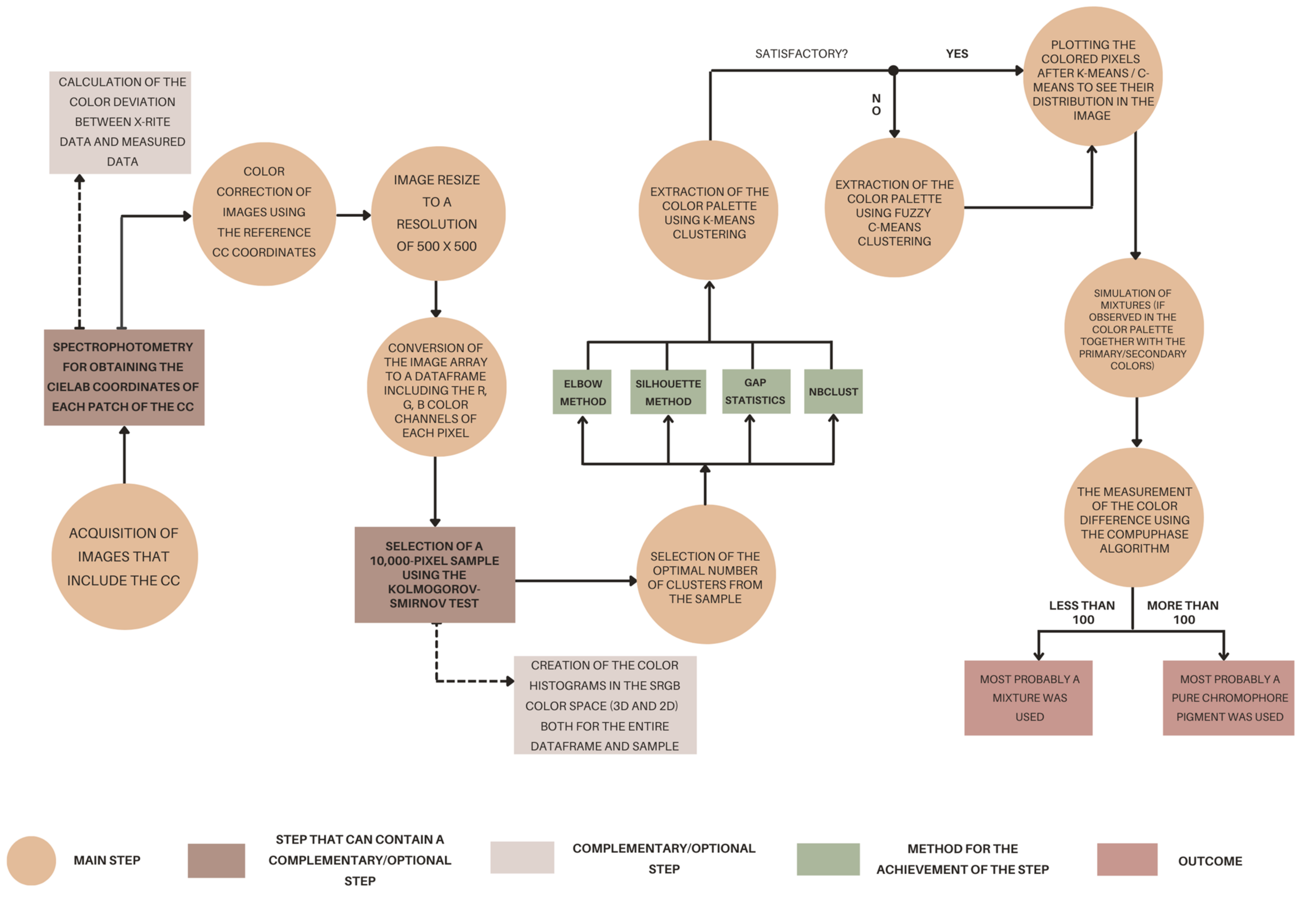
2.2.8. Summarized Workflow
3. Results
3.1. The Pigments and Binding Media Used in the Paints of Boris Brollo
3.1.1. White Paint
3.1.2. Blue Paint
3.1.3. Red Paint
3.1.4. Yellow Paint
3.1.5. Green Paint
3.1.6. Brown Paint
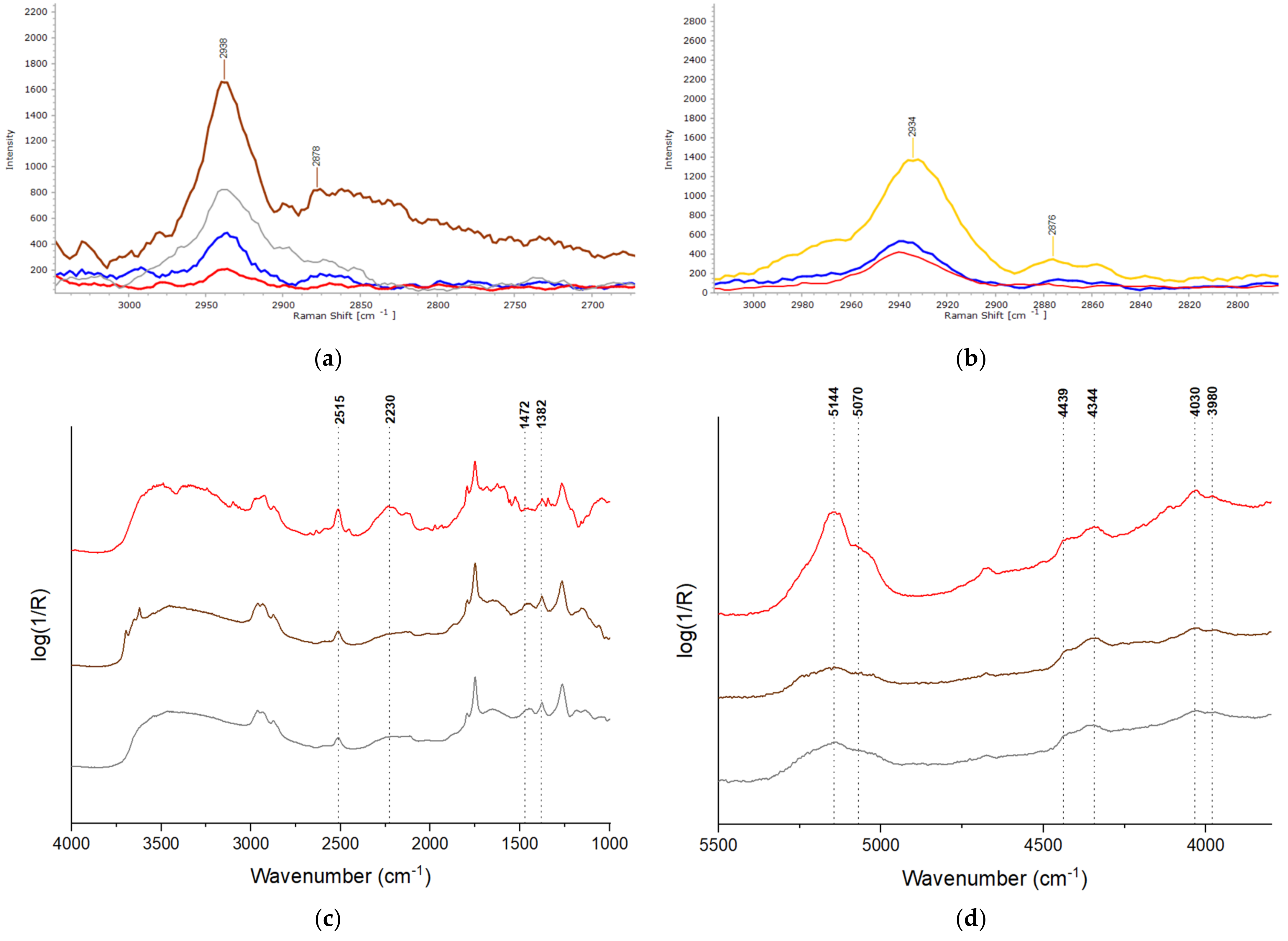
3.1.7. Binding Media
3.1.8. The Technique of Boris Brollo
3.2. The Application of the Proposed Computational Workflow
3.2.1. The Color Correction of the Images
3.2.2. The Selected pixel Samples and Their Color Histograms
3.2.3. The Selection of the Number of Clusters
3.2.4. The Extracted Color Palettes Using K-Means and Fuzzy C-Means Clustering
3.2.5. The Simulated Mixtures and the Measurement of the Color Difference
4. Conclusions
Author Contributions
Funding
Institutional Review Board Statement
Informed Consent Statement
Data Availability Statement
Acknowledgments
Conflicts of Interest
Appendix A


References
- Izzo, F.C.; Vitale, V.; Fabbro, C.; Van Keulen, H. Multi-Analytical Investigation on Felt-Tip Pen Inks: Formulation and Preliminary Photo-Degradation Study. Microchem. J. 2016, 124, 919–928. [Google Scholar] [CrossRef]
- Kwon, H.; Lee, G. Collaboration with Stakeholders for Conservation of Contemporary Art. J. Conserv. Sci. 2020, 36, 37–46. [Google Scholar] [CrossRef] [Green Version]
- Kampasakali, E.; Fardi, T.; Pavlidou, E.; Christofilos, D. Towards Sustainable Museum Conservation Practices: A Study on the Surface Cleaning of Contemporary Art and Design Objects with the Use of Biodegradable Agents. Heritage 2021, 4, 2023–2043. [Google Scholar] [CrossRef]
- Macchia, A.; Biribicchi, C.; Carnazza, P.; Montorsi, S.; Sangiorgi, N.; Demasi, G.; Prestileo, F.; Cerafogli, E.; Colasanti, I.A.; Aureli, H.; et al. Multi-Analytical Investigation of the Oil Painting “Il Venditore Di Cerini” by Antonio Mancini and Definition of the Best Green Cleaning Treatment. Sustainability 2022, 14, 3972. [Google Scholar] [CrossRef]
- Szmelter, I. New Values of Cultural Heritage and the Need for a New Paradigm Regarding its Care. CeROArt Conservation Exposition Restauration d’Objets d’Art. 2013. Available online: https://journals.openedition.org/ceroart/3647 (accessed on 12 June 2023).
- Luca, G.D.; Dastgerdi, A.S.; Francini, C.; Liberatore, G. Sustainable Cultural Heritage Planning and Management of Overtourism in Art Cities: Lessons from Atlas World Heritage. Sustainability 2020, 12, 3929. [Google Scholar] [CrossRef]
- Cosentino, A. Identification of Pigments by Multispectral Imaging; a Flowchart Method. Herit. Sci. 2014, 2, 8. [Google Scholar] [CrossRef] [Green Version]
- Cosentino, A.; Stout, S. Photoshop and Multispectral Imaging for Art Documentation. e-Preserv. Sci. 2014, 11, 91–98. [Google Scholar]
- Cosentino, A. Multispectral Imaging of Pigments with a Digital Camera and 12 Interferential Filters. e-Preserv. Sci. 2015, 12, 1–7. [Google Scholar]
- Sáez-Hernández, R.; Antela, K.U.; Gallello, G.; Cervera, M.L.; Mauri-Aucejo, A.R. A Smartphone-Based Innovative Approach to Discriminate Red Pigments in Roman Frescoes Mock-Ups. J. Cult. Herit. 2022, 58, 156–166. [Google Scholar] [CrossRef]
- Manfredi, E.; Petrillo, G.; Dellepiane, S. A Novel Digital-Camera Characterization Method for Pigment Identification in Cultural Heritage. In Computational Color Imaging; Tominaga, S., Schettini, R., Trémeau, A., Horiuchi, T., Eds.; Springer International Publishing: Cham, Switzerland, 2019; Volume 11418, pp. 195–206. ISBN 978-3-030-13939-1. [Google Scholar]
- Molada-Tebar, A.; Lerma, J.L.; Marqués-Mateu, Á. Camera Characterization for Improving Color Archaeological Documentation. Color Res. Appl. 2018, 43, 47–57. [Google Scholar] [CrossRef]
- Trombini, M.; Ferraro, F.; Manfredi, E.; Petrillo, G.; Dellepiane, S. Camera Color Correction for Cultural Heritage Preservation Based on Clustered Data. J. Imaging 2021, 7, 115. [Google Scholar] [CrossRef]
- Izzo, F.C.; Perusini, G.; Le Tempere Di De Maria, Laurenti, Cadorin, Favai e Casorati: Riscontri Tra Documenti d’archivio, Prove Di Ricostruzione e Analisi Scientifiche, in T. Perusini (a Cura Di), Tecnica Della Pittura in Italia Fra Ottocento e Novecento, Atti Del Convegno, Venezia 23/03/19, Sargon, Padova 2021, pp.125–149. Tecnica Della Pittura in Italia fra Ottocento e Novecento 2021. Available online: https://www.academia.edu/49398757/Le_tempere_di_De_Maria_Laurenti_Cadorin_Favai_e_Casorati_riscontri_tra_documenti_d_archivio_prove_di_ricostruzione_e_analisi_scientifiche_in_T_Perusini_a_cura_di_Tecnica_della_pittura_in_Italia_fra_Ottocento_e_Novecento_atti_del_convegno_Venezia_23_03_19_Sargon_Padova_2021_pp_125_149 (accessed on 12 June 2023).
- Morales Toledo, E.G.; Raicu, T.; Falchi, L.; Barisoni, E.; Piccolo, M.; Izzo, F.C. Critical Analysis of the Materials Used by the Venetian Artist Guido Cadorin (1892–1976) during the Mid-20th Century, Using a Multi-Analytical Approach. Heritage 2023, 6, 600–627. [Google Scholar] [CrossRef]
- De la Rie, E.R. Old Master Paintings: A Study of the Varnish Problem. Anal. Chem. 1989, 61, 1228A–1240A. [Google Scholar] [CrossRef]
- Simonot, L.; Elias, M. Color Change Due to a Varnish Layer. Color Res. Appl. 2004, 29, 196–204. [Google Scholar] [CrossRef]
- Stringa, N. Pittura Nel Veneto. Il Novecento. Dizionario Degli Artisti; La pittura nel Veneto; Edizione Illustrata; Mondadori Electa: Roma, Italy, 2009. [Google Scholar]
- Piccolo, A.; Bonato, E.; Falchi, L.; Lucero-Gómez, P.; Barisoni, E.; Piccolo, M.; Balliana, E.; Cimino, D.; Izzo, F.C. A Comprehensive and Systematic Diagnostic Campaign for a New Acquisition of Contemporary Art—The Case of Natura Morta by Andreina Rosa (1924–2019) at the International Gallery of Modern Art Ca’ Pesaro, Venice. Heritage 2021, 4, 4372–4398. [Google Scholar] [CrossRef]
- Raicu, T.; Zollo, F.; Falchi, L.; Barisoni, E.; Piccolo, M.; Izzo, F.C. Preliminary Identification of Mixtures of Pigments Using the PaletteR Package in R—The Case of Six Paintings by Andreina Rosa (1924–2019) from the International Gallery of Modern Art Ca’ Pesaro, Venice. Heritage 2023, 6, 524–547. [Google Scholar] [CrossRef]
- Biografia Di Boris Brollo. Available online: http://www.lavocedelcittadino.net/files/BIOGRAFIA_DI_BORIS_BROLLO_.pdf (accessed on 22 May 2023).
- Russell, J.; Singer, B.W.; Perry, J.J.; Bacon, A. The Identification of Synthetic Organic Pigments in Modern Paints and Modern Paintings Using Pyrolysis-Gas Chromatography–Mass Spectrometry. Anal. Bioanal. Chem. 2011, 400, 1473–1491. [Google Scholar] [CrossRef]
- Kirchner, E. Instrumental Colour Mixing to Guide Oil Paint Artists. J. Int. Colour Assoc. 2019, 24, 24–34. [Google Scholar]
- SOPRANO. Available online: https://soprano.kikirpa.be/ (accessed on 26 March 2023).
- Guidelines: Technical Guidelines for Digitizing Cultural Heritage Materials—Federal Agencies Digital Guidelines Initiative. Available online: https://www.digitizationguidelines.gov/guidelines/digitize-technical.html (accessed on 30 April 2022).
- ColorChecker Classic Mini. Available online: https://calibrite.com/product/colorchecker-classic-mini/ (accessed on 30 April 2022).
- Molada, A.; Marqués-Mateu, A.; Lerma, J.; Westland, S. Dominant Color Extraction with K-Means for Camera Characterization in Cultural Heritage Documentation. Remote Sens. 2020, 12, 520. [Google Scholar] [CrossRef] [Green Version]
- Imatest Version 2021.2. Available online: https://www.imatest.com/micro_site/2021-2/ (accessed on 28 November 2022).
- Sharma, G.; Wu, W.; Dalal, E.N. The CIEDE2000 Color-Difference Formula: Implementation Notes, Supplementary Test Data, and Mathematical Observations. Color Res. Appl. 2005, 30, 21–30. [Google Scholar] [CrossRef]
- Ialenti, A. Clustering Pollock. Available online: https://towardsdatascience.com/clustering-pollock-1ec24c9cf447 (accessed on 4 July 2022).
- Adobe Express. Available online: https://express.adobe.com/tools/image-resize (accessed on 2 October 2022).
- Walker, R. Color Quantization in R—R-Bloggers. Available online: https://www.r-bloggers.com/2016/01/color-quantization-in-r/ (accessed on 22 May 2023).
- Malato, G. How to Correctly Select a Sample from a Huge Dataset in Machine Learning. Data Science Reporter 2019; Kdnuggets: Brooklin, MA, USA, 2019. [Google Scholar]
- Nanjundan, S.; Sankaran, S.; Arjun, C.R.; Anand, G.P. Identifying the Number of Clusters for K-Means: A Hypersphere Density Based Approach. arXiv 2019, arXiv:1912.00643. [Google Scholar] [CrossRef]
- Cui, M. Introduction to the K-Means Clustering Algorithm Based on the Elbow Method. Account. Audit. Financ. 2020, 1, 5–8. [Google Scholar]
- Hastie, T.; Tibshirani, R.; Friedman, J. The Elements of Statistical Learning, 2nd ed.; Springer Series in Statistics; Springer: New York, NY, USA, 2009; ISBN 978-0-387-84857-0. [Google Scholar]
- Charrad, M.; Ghazzali, N.; Boiteau, V.; Niknafs, A. NbClust: An R Package for Determining the Relevant Number of Clusters in a Data Set. J. Stat. Softw. 2014, 61, 1–36. [Google Scholar] [CrossRef] [Green Version]
- Package “Cluster”. Available online: https://cran.r-project.org/web/packages/cluster/cluster.pdf (accessed on 22 May 2023).
- Wang, F.; Franco-Penya, H.-H.; Kelleher, J.D.; Pugh, J.; Ross, R. An Analysis of the Application of Simplified Silhouette to the Evaluation of K-Means Clustering Validity. In Machine Learning and Data Mining in Pattern Recognition; Perner, P., Ed.; Lecture Notes in Computer Science; Springer International Publishing: Cham, Switzerland, 2017; Volume 10358, pp. 291–305. ISBN 978-3-319-62415-0. [Google Scholar]
- Weller, H. Package ‘Colordistance’. Available online: https://cran.r-project.org/web/packages/colordistance/colordistance.pdf (accessed on 22 May 2023).
- Murdoch, D. Package “Rgl”. Available online: https://cran.r-project.org/web/packages/rgl/rgl.pdf (accessed on 22 May 2023).
- Zhang, W.; Dong, L.; Pan, X.; Zou, P.; Qin, L.; Xu, W. A Survey of Restoration and Enhancement for Underwater Images. IEEE Access 2019, 7, 182259–182279. [Google Scholar] [CrossRef]
- Buades, A.; Lisani, J.-L.; Morel, J.-M. Dimensionality of Color Space in Natural Images. J. Opt. Soc. Am. A JOSAA 2011, 28, 203–209. [Google Scholar] [CrossRef]
- Mohanty, A.; Rajkumar, S.; Muzaffar Mir, Z.; Bardhan, P. Analysis of Color Images Using Cluster Based Segmentation Techniques. Int. J. Comput. Appl. 2013, 79, 42–47. [Google Scholar] [CrossRef]
- Nayak, J.; Naik, B.; Behera, H.S. Fuzzy C-Means (FCM) Clustering Algorithm: A Decade Review from 2000 to 2014. Comput. Intell. Data Min. 2014, 2, 133. [Google Scholar]
- Dhanachandra, N.; Manglem, K.; Chanu, Y.J. Image Segmentation Using K -Means Clustering Algorithm and Subtractive Clustering Algorithm. Procedia Comput. Sci. 2015, 54, 764–771. [Google Scholar] [CrossRef] [Green Version]
- Wu, J. Cluster Analysis and K-Means Clustering: An Introduction. In Advances in K-Means Clustering: A Data Mining Thinking; Wu, J., Ed.; Springer Theses; Springer: Berlin/Heidelberg, Germany, 2012; pp. 1–16. ISBN 978-3-642-29807-3. [Google Scholar]
- Jipkate, B.R.; Gohokar, V.V. A Comparative Analysis of Fuzzy C-Means Clustering and K Means Clustering Algorithms. Int. J. Comput. Eng. Res. 2012, 2, 737–739. [Google Scholar]
- R: The R Stats Package. Available online: https://stat.ethz.ch/R-manual/R-devel/library/stats/html/00Index.html (accessed on 24 September 2022).
- Meyer, D. Package ‘E1071’. Available online: https://cran.r-project.org/web/packages/e1071/e1071.pdf (accessed on 22 May 2023).
- Kurosu, M. Human-Computer Interaction. Theories, Methods, and Human Issues. In Proceedings of the 20th International Conference, HCI International 2018, Las Vegas, NV, USA, 15–20 July 2018; Part I. Springer: Berlin/Heidelberg, Germany, 2018. ISBN 978-3-319-91238-7. [Google Scholar]
- Ilyas, A.; Farid, M.S.; Khan, M.H.; Grzegorzek, M. Exploiting Superpixels for Multi-Focus Image Fusion. Entropy 2021, 23, 247. [Google Scholar] [CrossRef] [PubMed]
- Colour Metric. Available online: https://www.compuphase.com/cmetric.htm (accessed on 14 April 2022).
- Kotsarenko, Y.; Ramos, F. Measuring Perceived Color Difference Using YIQ NTSC Transmission Color Space in Mobile Applications. Program. Mat. Softw. 2010, 2, 91. [Google Scholar]
- Gama, J. Package ‘Colorscience’. Available online: https://cran.r-project.org/web/packages/colorscience/colorscience.pdf (accessed on 22 May 2023).
- Maftei, A.E.; Buzatu, A.; Damian, G.; Buzgar, N.; Dill, H.G.; Apopei, A.I. Micro-Raman—A Tool for the Heavy Mineral Analysis of Gold Placer-Type Deposits (Pianu Valley, Romania). Minerals 2020, 10, 988. [Google Scholar] [CrossRef]
- Zendri, E.; Izzo, F.C.; Balliana, E.; Pinton, F. A Preliminary Study of the Composition of Commercial Oil, Acrylic and Vinyl Paints and Their Behaviour after Accelerated Ageing Conditions. Conserv. Sci. Cult. Herit. 2015, 14, 353–369. [Google Scholar]
- Fardi, T.; Pintus, V.; Kampasakali, E.; Pavlidou, E.; Schreiner, M.; Kyriacou, G. Analytical Characterization of Artist’s Paint Systems Based on Emulsion Polymers and Synthetic Organic Pigments. J. Anal. Appl. Pyrolysis 2018, 135, 231–241. [Google Scholar] [CrossRef]
- Osticioli, I.; Mendes, N.F.C.; Nevin, A.; Gil, F.P.S.C.; Becucci, M.; Castellucci, E. Analysis of Natural and Artificial Ultramarine Blue Pigments Using Laser Induced Breakdown and Pulsed Raman Spectroscopy, Statistical Analysis and Light Microscopy. Spectrochim. Acta Part A: Mol. Biomol. Spectrosc. 2009, 73, 525–531. [Google Scholar] [CrossRef] [PubMed] [Green Version]
- Deneckere, A.; De Reu, M.; Martens, M.P.J.; De Coene, K.; Vekemans, B.; Vincze, L.; De Maeyer, P.; Vandenabeele, P.; Moens, L. The Use of a Multi-Method Approach to Identify the Pigments in the 12th Century Manuscript Liber Floridus. Spectrochim. Acta Part A Mol. Biomol. Spectrosc. 2011, 80, 125–132. [Google Scholar] [CrossRef] [PubMed]
- Bakovic, M.; Karapandza, S.; Mcheik, S.; Pejović-Milić, A. Scientific Study of the Origin of the Painting from the Early 20th Century Leads to Pablo Picasso. Heritage 2022, 5, 1120–1140. [Google Scholar] [CrossRef]
- Colombini, A.; Kaifas, D. Characterization of some orange and yellow organic and fluorescent pigments by raman spectroscopy. e-Preserv. Sci. 2010, 7, 14–21. [Google Scholar]
- Defeyt, C.; Strivay, D. PB15 as 20th and 21st Artists’ Pigments: Conservation Concerns. e-Preserv. Sci. 2014, 11, 6–14. [Google Scholar]
- França De Sá, S.; Viana, C.; Ferreira, J.L. Tracing Poly(Vinyl Acetate) Emulsions by Infrared and Raman Spectroscopies: Identification of Spectral Markers. Polymers 2021, 13, 3609. [Google Scholar] [CrossRef]
- Miliani, C.; Rosi, F.; Daveri, A.; Brunetti, B.G. Reflection Infrared Spectroscopy for the Non-Invasive in Situ Study of Artists’ Pigments. Appl. Phys. A Mater. Sci. Process. 2012, 106, 295–307. [Google Scholar] [CrossRef]
- Rosi, F.; Daveri, A.; Moretti, P.; Brunetti, B.G.; Miliani, C. Interpretation of Mid and Near-Infrared Reflection Properties of Synthetic Polymer Paints for the Non-Invasive Assessment of Binding Media in Twentieth-Century Pictorial Artworks. Microchem. J. 2016, 124, 898–908. [Google Scholar] [CrossRef]
- Ferreira, J.L.; Melo, M.J.; Ramos, A.M. Poly(Vinyl Acetate) Paints in Works of Art: A Photochemical Approach. Part 1. Polym. Degrad. Stab. 2010, 95, 453–461. [Google Scholar] [CrossRef]
- Janakkumar Baldevbhai, P.; Anand, R.S. Color Image Segmentation for Medical Images Using L*a*b* Color Space. IOSR J. Electron. Commun. Eng. (IOSRJECE) 2012, 1, 24–45. [Google Scholar] [CrossRef]
- Kirchner, E.; van Wijk, C.; van Beek, H.; Koster, T. Exploring the Limits of Color Accuracy in Technical Photography. Herit. Sci. 2021, 9, 57. [Google Scholar] [CrossRef]
- Color Correction Matrix (CCM)—Imatest. Available online: https://www.imatest.com/support/docs/pre-5-2/colormatrix/ (accessed on 22 May 2023).
- Ferraro, M.B. Cluster Analysis. Available online: https://web.uniroma1.it/memotef/sites/default/files/file%20lezioni/Clustering.pdf (accessed on 22 May 2023).
- Löhr, T. K-Means Clustering and the Gap-Statistics. Available online: https://towardsdatascience.com/k-means-clustering-and-the-gap-statistics-4c5d414acd29 (accessed on 22 May 2023).
- ColorChecker Passport User Manual. Available online: https://www.xrite.com/-/media/xrite/files/manuals_and_userguides/c/o/colorcheckerpassport_user_manual_en.pdf (accessed on 22 May 2023).


| Variable | Value |
|---|---|
| Flash | Off |
| ISO | 400 |
| Operation Mode | Manual |
| Exposure Time | 1/125 |
| Quality | RAW |
| F-stop | 1.0 |
| Color Space | sRGB |
| Variable | Value |
|---|---|
| Optimize | ΔE00 |
| Type of Matrix | 3 × 3 |
| Linearization | Gamma polynomial data fit |
| Weighting | Using the L* color coordinate (which represents lightness) |
| Optimization Constraint | No constraints |
| Type of Calculation | Estimation of input RGB values, calculation of the XYZ matrix and xy primaries, and conversion to output RGB values. |
| Chroma Multiplier | The default value of 1 was kept. |
| Paint Color | Main Constituents | Band Wavenumber (cm−1) |
|---|---|---|
| Blue | Ultramarine blue | 547 s |
| Titanium white (Rutile) | 447 m, 611 m | |
| Gypsum | 1007 w | |
| Calcite | 1087 w | |
| White | Titanium white (Rutile) | 447 s, 611 s |
| Gypsum | 1009 m | |
| Calcite | 1087 m | |
| Yellow | Monoazo yellow pigment | 358 w, 389 w, 509 w, 785 m, 823 w, 949 w, 998 m, 1137 m, 1216 m, 1254 m, 1310 s, 1337 m, 1386 m, 1448 w, 1484 vs, 1534 w, 1562 w, 1619 s, 1670 w |
| Titanium white (Rutile) | 447 s, 611 s | |
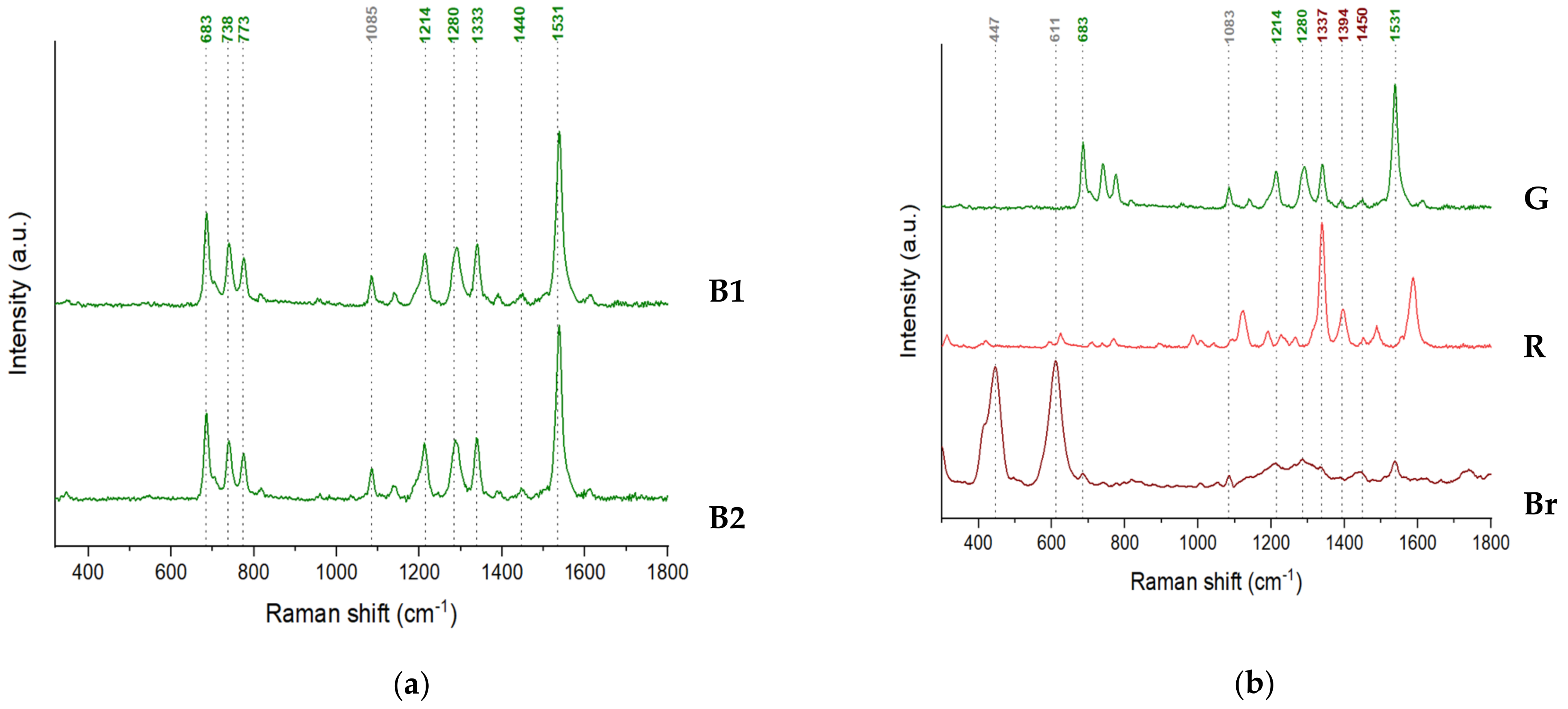
| Green | Phthalocyanine green (PG7) | 683 s, 738 m, 773 m, 1214 m, 1280 m, 1333 m, 1440 w, 1531 s |
| Calcite | 1085 w | |
| Red | Pigment Red 4 (PR4) | 421 w, 593 w, 626 w, 708 w, 767 w, 892 w, 985 w, 1095 w, 1123 m, 1181 w, 1224 w, 1266 w, 1337 vs, 1397 m, 1452 w, 1485 w, 1553 w, 1586 s |
| Gypsum | 1010 w | |
| Brown (present only in B1) | Pigment Red 4 (PR4) and phthalocyanine green (PG7) | 683 w, 1214 w, 1280 m, 1531 w (these peaks are characteristic to PG7), 1337 w, 1394 w, 1450 w (might be characteristic to both PG7 and PR4) |
| Titanium white (Rutile) | 447 s, 611 s |
| ΔE2000 (corrected-reference) (Guido Cadorin’s paintings) | 4.77 |
| ΔE2000 (corrected-reference) (Andreina Rosa’s paintings) | 3.68 |
| ΔE2000 (corrected-reference) (Boris Brollo’s paintings) | 3.59 |
| Painting Index | Number of Clusters (Elbow Method) | Number of Clusters (Silhouette Method) | Number of Clusters (Gap Statistic Method) | The Final Selected Number of Clusters |
|---|---|---|---|---|
| C1 | 5 | 2 | 9 | 6 |
| C2 | 4 | 2 | 6 | 7 |
| C3 | 6 | 2 | 2 | 8 |
| C4 | 5 | 2 | 5 | 3 |
| C5 | 7 | 2 | 3 | 7 |
| C6 | 5 | 3 | 11 | 10 |
| C7 | 7 | 3 | 1 | 4 |
| R1 | 5 | 2 | 1 | 15 |
| R2 | 8 | 2 | 4 | 6 |
| R3 | 6 | 2 | 1 | 12 |
| R4 | 6 | 2 | 3 | 8 |
| R5 | 9 | 2 | 14 | 12 |
| R6 | 6 | 3 | 4 | 8 |
| B1 | 7 | 9 | 6 | 9 |
| B2 | 6 | 9 | 8 | 7 |
| B3 | 8 | 7 | 7 | 7 |
| Painting Index | Mixed Colors | Color to be Achieved | Percentage of Colors in the Mixture | CompuPhase Color Difference (Colors Extracted Using K-Means Clustering) | CompuPhase Color Difference (Colors Extracted Using Fuzzy C-Means Clustering) |
|---|---|---|---|---|---|
| R1 | blue and red | purple | 50% blue + 50% red | 24.01 | 11.59 |
| 60% blue + 40% red | 4.26 | 1.76 | |||
| 70% blue + 30% red | 17.42 | 13.64 | |||
| 80% blue + 20% red | 37.38 | 26.29 | |||
| R3 | blue and yellow | green | 40% blue + 60% yellow | 53.21 | 34.4 |
| 50% blue + 50% yellow | 37.33 | 31.91 | |||
| 60% blue + 40% yellow | 31.02 | 43.54 | |||
| 70% blue + 30% yellow | 38.97 | 61.61 | |||
| red and blue | purple | 40% red + 60% blue | 54.71 | 45.28 | |
| 50% red + 50% blue | 52.37 | 44.60 | |||
| 60% red + 40% blue | 52.63 | 46.50 | |||
| 70% red + 30% blue | 55.45 | 50.70 | |||
| R5 | red and green | brown | 50% red + 50% green | 51.92 | 37.34 |
| 60% red + 40% green | 56.48 | 43.10 | |||
| 70% red + 30% green | 61.96 | 49.97 | |||
| 80% red + 20% green | 68.15 | 57.58 | |||
| R6 | red and blue | purple | 50% red + 50% blue | 52.15 | 30.97 |
| 60% red + 40% blue | 49.98 | 29.54 | |||
| 70% red + 30% blue | 50.58 | 32.18 | |||
| 80% red + 20% blue | 53.83 | 38.03 | |||
| B1 | red and green | brown | 50% red + 50% green | 51.68 | 64.6 |
| 60% red + 40% green | 28.19 | 38.7 | |||
| 70% red + 30% green | 52.12 | 54.93 | |||
| 80% red + 20% green | 93.42 | 95.37 | |||
| yellow and blue | green | 30% yellow and 70% blue | 124.4 | 130.03 | |
| 40% yellow and 60% blue | 120.4 | 147.6 | |||
| 50% yellow and 50% blue | 144.53 | 186.02 | |||
| 60% yellow and 40% blue | 186.7 | 235.74 | |||
| B2 | yellow and blue | green | 30% yellow and 70% blue | 127.13 | 127.48 |
| 40% yellow and 60% blue | 125.61 | 126.2 | |||
| 50% yellow and 50% blue | 148.14 | 148.75 | |||
| 60% yellow and 40% blue | 186.96 | 187.44 | |||
| B3 | yellow and blue | green | 30% yellow and 70% blue | 126.48 | 147.25 |
| 40% yellow and 60% blue | 125.57 | 165.52 | |||
| 50% yellow and 50% blue | 149.07 | 200.29 | |||
| 60% yellow and 40% blue | 188.86 | 245.24 |
Disclaimer/Publisher’s Note: The statements, opinions and data contained in all publications are solely those of the individual author(s) and contributor(s) and not of MDPI and/or the editor(s). MDPI and/or the editor(s) disclaim responsibility for any injury to people or property resulting from any ideas, methods, instructions or products referred to in the content. |
© 2023 by the authors. Licensee MDPI, Basel, Switzerland. This article is an open access article distributed under the terms and conditions of the Creative Commons Attribution (CC BY) license (https://creativecommons.org/licenses/by/4.0/).
Share and Cite
Raicu, T.; Zollo, F.; Falchi, L.; Barisoni, E.; Piccolo, M.; Izzo, F.C. Towards a More Sustainable and Less Invasive Approach for the Investigation of Modern and Contemporary Paintings. Sustainability 2023, 15, 12197. https://doi.org/10.3390/su151612197
Raicu T, Zollo F, Falchi L, Barisoni E, Piccolo M, Izzo FC. Towards a More Sustainable and Less Invasive Approach for the Investigation of Modern and Contemporary Paintings. Sustainability. 2023; 15(16):12197. https://doi.org/10.3390/su151612197
Chicago/Turabian StyleRaicu, Teodora, Fabiana Zollo, Laura Falchi, Elisabetta Barisoni, Matteo Piccolo, and Francesca Caterina Izzo. 2023. "Towards a More Sustainable and Less Invasive Approach for the Investigation of Modern and Contemporary Paintings" Sustainability 15, no. 16: 12197. https://doi.org/10.3390/su151612197