Energy Management Systems for Smart Electric Railway Networks: A Methodological Review

Abstract

Energy shortage is one of the major concerns in today’s world. As a consumer of electrical energy, the electric railway system (ERS), due to trains, stations, and commercial users, intakes an enormous amount of electricity. Increasing greenhouse gases (GHG) and CO₂ emissions, in addition, have drawn the regard of world leaders as among the most dangerous threats at present; based on research in this field, the transportation sector contributes significantly to this pollution. Railway Energy Management Systems (REMS) are a modern green solution that not only tackle these problems but also, by implementing REMS, electricity can be sold to the grid market. Researchers have been trying to reduce the daily operational costs of smart railway stations, mitigating power quality issues, considering the traction uncertainties and stochastic behavior of Renewable Energy Resources (RERs) and Energy Storage Systems (ESSs), which has a significant impact on total operational cost. In this context, the first main objective of this article is to take a comprehensive review of the literature on REMS and examine closely all the works that have been carried out in this area, and also the REMS architecture and configurations are clarified as well. The secondary objective of this article is to analyze both traditional and modern methods utilized in REMS and conduct a thorough comparison of them. In order to provide a comprehensive analysis in this field, over 120 publications have been compiled, listed, and categorized. The study highlights the potential of leveraging RERs for cost reduction and sustainability. Evaluating factors including speed, simplicity, efficiency, accuracy, and ability to handle stochastic behavior and constraints, the strengths and limitations of each optimization method are elucidated.

1. Introduction

1.1. Motivation

Increasing greenhouse gas (GHG) emissions is one of the biggest concerns of world decision-makers. As a result of their contribution to air pollution and the release of greenhouse gases (GHGs) and carbon dioxide (CO₂) [1], modern transport systems contribute significantly to environmental impacts. A total of 93.2% of the sector’s emissions are caused by road transport, making up 28.3% of the total energy-related CO₂ emissions in the EU28 [2]. In addition, GHG emissions are predicted to be 28% in 2050 [3]. Greener travel behaviors, can be promoted to reduce congestion and pollution through the introduction of encouragements for the adoption of low-emission alternative energies and vehicles, using public transportation, and implementing bicycle and car-sharing/pooling schemes [4].

Many countries and cities rely heavily on rail-based passenger transportation [5]. Despite producing 3.6% of global transport emissions and consuming 2.1% of global transport energy, rail is considered one of the cleanest modes of transportation [6,7]. Despite increased global CO₂ emissions, railways are one of the few transportation modes with decreasing CO₂ emissions. Japan and the UK have reduced greenhouse gas emissions by encouraging and improving low-carbon rail, including electric trains (ETs) and hydrogen trains (HTs).

Energy shortages and the contradictory nature of economic growth become increasingly evident as the world’s economy continues to expand and demand for energy increases. As many public buildings serve, at present, multiple functions, energy consumption is also high, especially in a society with an information economy [8]. Increasing populations, industries, and services require large-scale transportation [9]. Railway stations are large public buildings that have the following characteristics: automation of public buildings, modernization of communication systems, office automation, building automation, etc. [10]. Indeed, the train itself consumes a great deal of energy as it moves and operates. Developing green energy, particularly renewable energy, to displace fossil fuels is particularly important, as is establishing a distributed smart energy station with a combination of photovoltaic and gas power generation systems together with energy storage technology, offering renewable sources of cold, heat, power, and water to new constructions, enabling them to achieve ultra-low or zero energy consumption [11]. Also, high-speed railway stations have high energy efficiency and could be utilized for generating energy from on-site renewable sources; for instance, by the usage of an integrated renewable energy source, an energy storage system (ESS), regenerative braking energy (RBE), and a power grid system are installed [12].

Energy management systems play a crucial role in optimizing the energy consumption and operational efficiency of railway systems and smart railway networks. With the growing emphasis on sustainable transportation solutions, railway operators are increasingly adopting advanced technologies to reduce energy consumption, minimize environmental impact, and enhance overall system performance. Energy management systems offer a comprehensive approach to monitor, control, and optimize energy usage in railway networks, ensuring efficient operations and the cost-effective utilization of resources.

Figure 1 serves as a valuable visual aid, illustrating the flowchart of this paper and facilitating a comprehensive understanding of the presented concepts.

1.2. Literature Review

In terms of energy consumption in ERS, the authors of reference [8] categorized the power consumption of a system in a railway station in China, as shown in Figure 2. The system consisted of six parts, each consuming a certain amount of power. To manage the energy efficiently, the authors applied the basic Railway Energy Management System (REMS). In this study, Energy Storage Systems (ESSs) in the form of batteries were utilized. The batteries were charged during off-peak hours, using the primary grid during the night when tariffs were low, and the PV panels installed in the station at no cost around noon when the panels produced a large amount of power. During peak hours, the batteries were discharged via the station grid, resulting in significant reductions in electricity costs.

The authors of reference [13] conducted a quarterly survey in Milan, Italy, to measure the active and reactive energy consumption at a railway station. The survey was conducted at fifteen-minute intervals for different seasons. Ref. [14] introduced a prototype implementation of an advanced automation architecture for electrical railway systems. The objective was to transform these systems into cyber-physical systems, enabling enhanced automation and control. As part of the prototype, two software suites were developed: the REM-S Offline Suite and the REM-S Online Suite. Ref. [15] conducted a critical analysis and case study on a Polish railway undertaking to identify methods for enhancing energy efficiency. The findings revealed that organizational measures were primarily responsible for the achieved energy efficiency improvements.

Most electric railways rely solely on pantograph-catenary systems for powering trains, which can lead to technical issues [16,17]. However, researchers have focused on increasing energy efficiency through the storage of regenerative braking energy on Energy Storage Systems (ESSs) [18]. The role of an Energy Storage System in urban railway systems, particularly stationary ultracapacitors and their uncertainties, was discussed in reference [19], where a strategy was outlined for optimizing energy management in wayside energy storage systems to maximize regenerative braking efficiency benefits. In reference [20], ESS and microgrid were proposed as hierarchical energy management strategies. An optimal operational strategy for ERSs can be developed based on the methodology developed by the authors of reference [21] to optimize costs along with renewable energy resources and regenerative braking energy.

The integration of metro and electric vehicles into a sustainable transportation system was analyzed in reference [22]. In reference [23], a DC microgrid incorporating PV, regenerative braking energy, and an ESS for charging electric vehicles near train stations was proposed. The paper examined power management and the effect of ESS size on conversion efficiency to maximize renewable energy utilization. However, renewable energy was only used for charging electric vehicles, and station loads and passengers’ changes were not considered. Ref. [24] suggested a charging method that utilizes regenerative braking energy from trains to recharge Electric Vehicle (EV) batteries. Additionally, the energy stored in the batteries can provide auxiliary power to trains during acceleration. Ref. [25] presented a study on integrating Electric Vehicle Parking lots (EVPLs) with Photovoltaic (PV) systems in railways to minimize line losses. The optimal management of EVPLs can reduce line losses and alleviate load flows. Refs. [26,27] modeled a region with metro, electric vehicles, and distributed generation, studying how to best utilize regenerative braking energy to power other trains or EVs. However, issues related to operating over the nominal power of traction transformers, economic operation problems, and charging units for electric buses were not addressed. Refs. [28,29] utilized travel profiles to optimize the energy consumption of electric vehicles. An energy management algorithm for a grid-connected EV charging park was presented in reference [30], but EV arrival and departure times were not included. Refs. [31,32] studied the integration of smart parking systems with RESs and EVs in a virtual microgrid. Ref. [33] proposed a hybrid algorithm for designing energy management systems, considering an artificial neural network and approximate dynamic programming. They also researched charging times of electric vehicles to reduce costs for EV parking lot owners.

Ref. [27] presented an integrated power management system that takes into account regenerative braking energy to integrate wind, solar, and electric vehicle charging infrastructures into MVDC railway microgrids. MVDC ERSs offer promising architectures for utilizing renewable energy sources and achieving sustainable transportation systems. An optimal sizing method for storage energy systems and an optimal method for traction power supply system operation for electric railways were developed in reference [34]. The control of electrical power over parallel power supply segments was made possible using an upgraded AC TPSS with power transfer devices in parallel with a neutral section [35]. Ref. [36] presented TPSS energy consumption optimization and power flow optimization using a hierarchical control model. Ref. [37] explored the coordination of distributed energy resources and electric urban transportation, as well as cost savings potential. Ref. [38] proposed an energy-saving and voltage-stabilizing control concept for reversible substations and storage systems. Ref. [39] introduced the integration of Digital Twin (DT) concepts into Electric Railway Power Systems (ERPSs), highlighting their importance in resolving ERPS issues. Ref. [24] focused on fuel cell hybrid locomotives (FCHL) and their components, including fuel cells, batteries, motors, and energy management systems, resulting in a reduction in hydrogen consumption. Ref. [40] presented several control strategies for ESS applications, including batteries, flywheels, and electric double-layer capacitors.

Optimization techniques have been explored in various domains like electric vehicles [41], but specific investigations and improvements are necessary for addressing the challenges and issues in railway systems. Surprisingly, no review paper dedicated to the application of Railway Energy Management Systems in RS optimization has been identified, indicating a gap in the existing literature. Accordingly, this review paper is prepared to make valuable scientific and practical contributions. Through a comprehensive literature review, it consolidates existing research on integrating renewable energy sources, EV charging structures, and optimization techniques in smart railways. The paper provides insights into integration architectures, highlighting the holistic approach needed to enhance energy efficiency. By exploring various optimization methods, their strengths, limitations, and applications, it guides future research and decision-making processes. The identification of challenges and opportunities, along with practical implications for implementation, offers valuable guidance to practitioners and decision-makers. Moreover, the focus on sustainability and environmental impact reinforces the potential of these systems to reduce carbon emissions and promote sustainable transportation solutions. Overall, this review paper significantly advances knowledge, informs decision-making, and supports the development of efficient and sustainable smart railway systems. It can provide a roadmap for experts and researchers, guiding future studies and method selection, particularly in the context of multi-objective and multi-functional optimization.

The subsequent sections of the paper are structured in the following manner: The Architecture of the REM-S Network is given in Section 3. In Section 4, the methodology and optimization methods are explained. In Section 5, the discussion and comparison, considering all the modern (practical) methods in the field of REMS, are presented. Finally, Section 6 concludes the paper with the overall remarks and results.

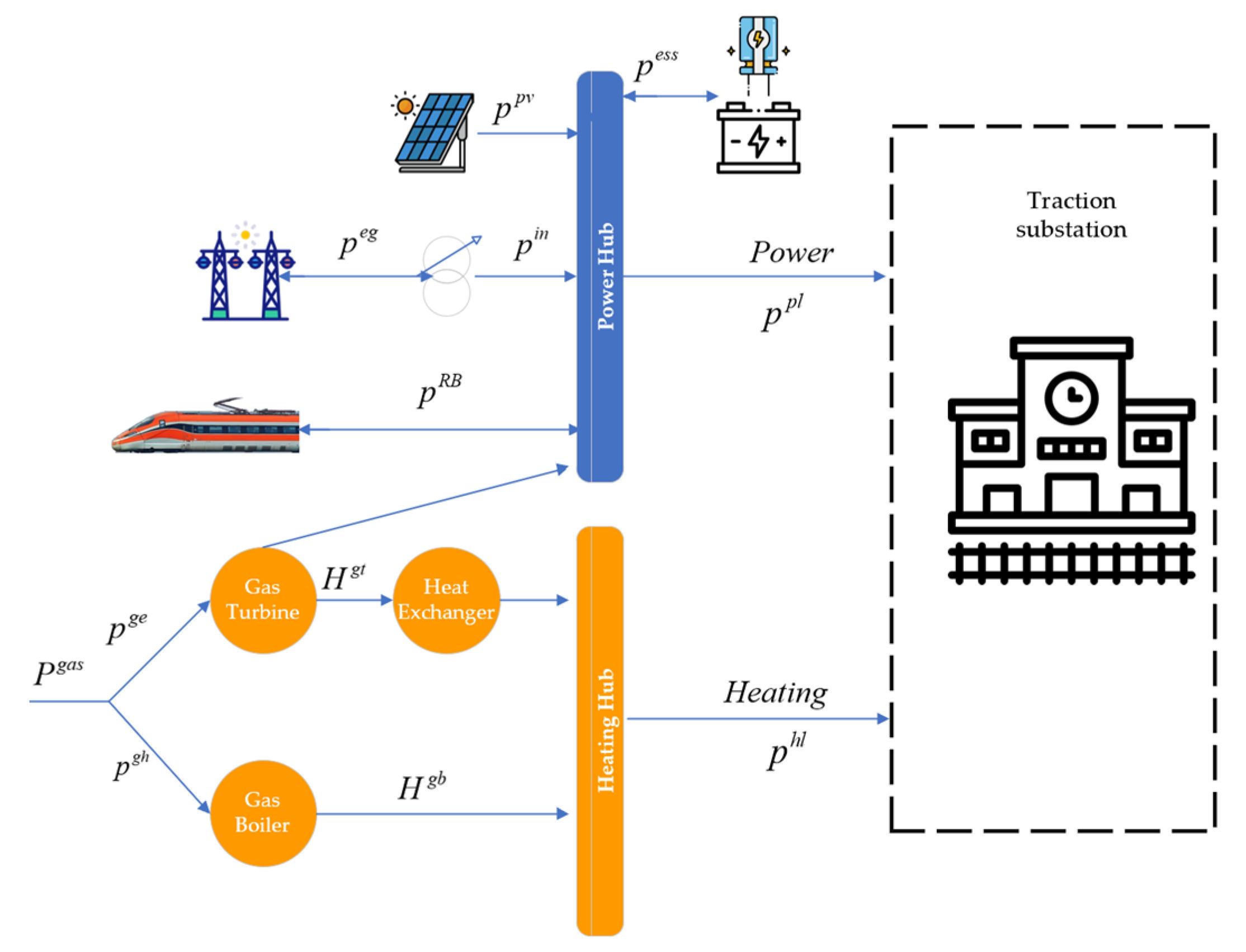
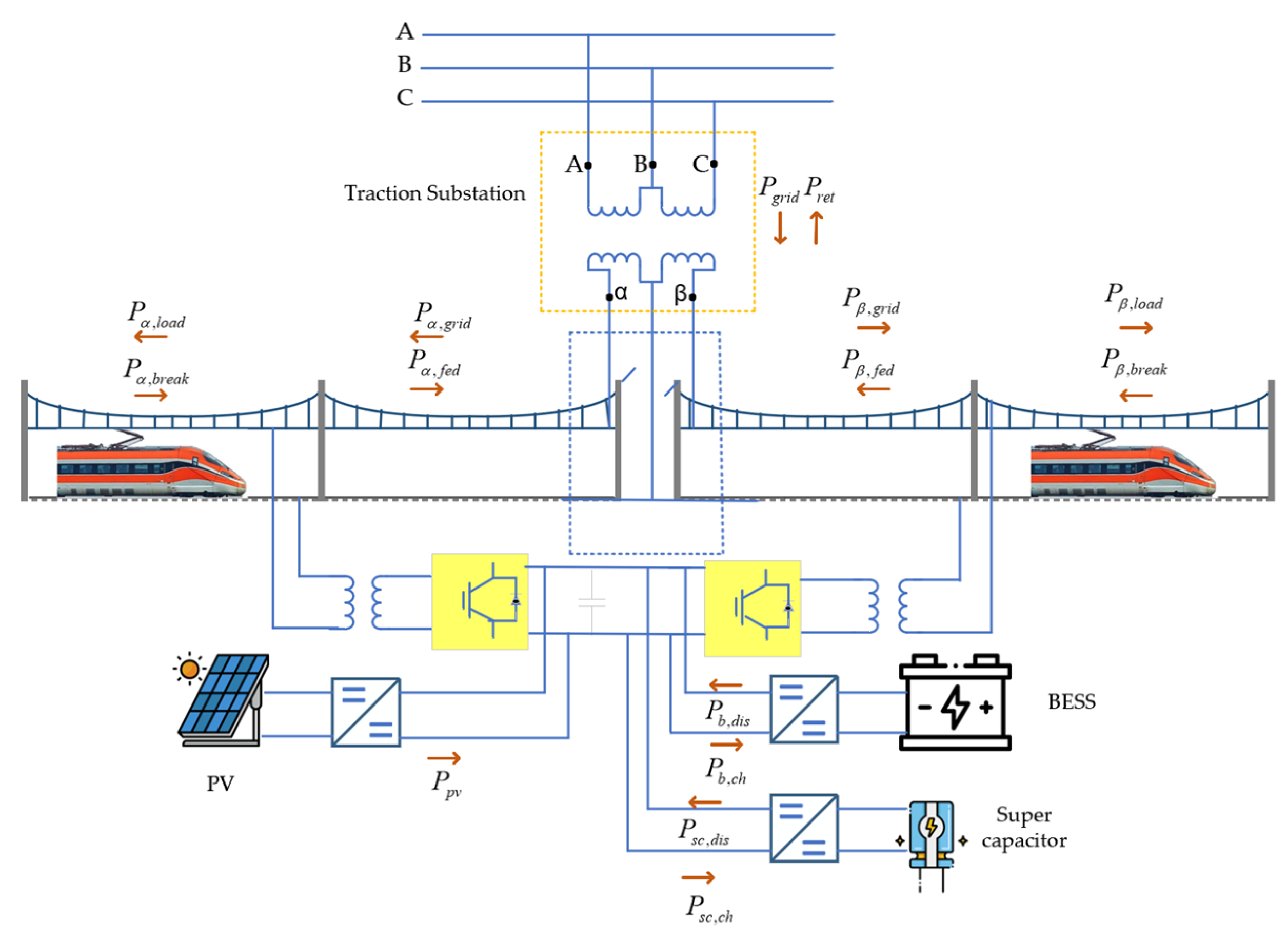
2. REMS Modeling Review

Ref. [42] presented an optimal energy management strategy using the MILP method. The strategy considers the actual installed capability of the rail system, including potential RBE and ESS, along with a PV generation unit in the parking area. The aim is to meet the demand for EV and electric bus charging spaces. A stochastic approach is used to account for uncertain EV behaviors and electricity market prices.

The proposed model shown in Figure 3, includes AC and DC fast charging units and addresses the energy needs of EVs purchased from the day-ahead market. The analysis examines the available capacity in lightly loaded railway transformers (150% power for two hours, based on EN50329 standard [43]) to meet parking lot charging demands and reduce infrastructure installation costs. Not considering PV, ESS, and RBE results in an approximately 80% increase in charging costs compared to the case where everything is considered. Thus, integrating RBE and ESS instead of PV systems reduces costs.

The study achieves a reliable power system by utilizing traction transformer power at its rated capacity. However, the study focuses on EV charging as the objective function and aims to minimize costs from day-ahead electricity markets through service and traction transformers. Train station energy use and train power demands are not taken into account, requiring expensive power supply from the main grid. Additionally, the study overlooks the waste of train regenerative braking energy due to train resistance, which represents a significant loss. Furthermore, wind turbines are not considered in this study.

Reference [44] proposes a heuristic mixed-integer linear programming model for railway station energy management. The model utilizes regenerative braking energy (RBE) and incorporates a stochastic approach. As shown in Figure 4, the study introduces a REMS model that includes an energy storage system (ESS), RBE utilization, a solar photovoltaic generator, and an external grid. The objective is to minimize the daily cost of electricity consumption at railway stations.

The paper explores bidirectional power flow, allowing the ESS and PV system to supply power back to the grid. Smart meters installed at the station provide the necessary communication infrastructure for the REMS to take dynamic action. Three pricing schemes are investigated, and the pricing signal significantly impacts the station’s daily operational cost. Additionally, the study considers the station’s internal demand, which is partially met using RBE obtained from trains. The calculated RBE is influenced by variations in passenger intensity throughout the day. The model also accounts for the stochastic nature of PV generation units.

The study highlights that the initial SOE of ESS and PV generation has a significant impact on grid power. By adopting a stochastic approach, the total daily operational cost of a smart railway station can be significantly reduced by utilizing ESS, PV, or a combination of ESS, PV, and RBE. Implementing the REMS model with dynamic pricing signals can lead to cost reductions of approximately 2–3%, even with ESS alone. Combining RBE, ESS, and PV proves to be the most efficient option, resulting in cost reductions of over 35%. However, it is worth noting that the study only considers the internal demand of the station, neglecting wind turbines, transformers, and the charging of electric cars and buses in EV parking lots.

Reference [45] presents an optimization study focused on a railroad electrical system that incorporates renewable energy resources (wind and solar PV systems), regenerative braking capabilities, and hybrid energy storage (batteries and supercapacitors) as shown in Figure 5. The uncertainties associated with wind and solar PV power are addressed using probability distribution functions. The optimization problem is solved using a differential evolution algorithm (DEA). The objective of the study is to minimize the total operating costs (TOC) of the railroad electrical system while considering various equality and inequality constraints. The amount of power produced by wind energy generators (WEGs) varies depending on wind speed, and the efficiency of solar PV is influenced by natural conditions such as solar irradiation and temperature.

The findings reveal that operating railroad electrical systems in a multi-source environment with RERs, regenerative braking, and hybrid storage systems leads to increased electrical energy returned to the main utility grid, resulting in significant cost reductions. However, the study does not account for uncertainties related to RBE, which is influenced by the number of passengers throughout the day and has a substantial impact on electricity production from RBE. Furthermore, the study does not explore train demand, station load consumption, EV charging, and the operation of transformers. These factors were not considered in the analysis.

In reference [46], optimal railway systems with regenerative braking are studied within the smart grid framework using a non-linear programming approach. The model incorporates renewable energy resources (RERs) like wind and solar PV power, along with electrical storage systems and supercapacitors. The aim is to enhance energy efficiency through regenerative braking and to optimize the design of railway electric infrastructure, including energy storage systems and reversible substations. The study shares similar characteristics with reference [45]. The results show that the incremental integration of RERs, electrical storage systems, and regenerative braking energy improves optimization and reduces the total operating cost (TOC). The simulation results also compare the performance of the GAMS solver for non-linear programming with the differential evolution algorithm (DEA). The GAMS v.24.1.3 software proves more effective in solving the optimization problem. However, the study overlooks the uncertainties related to regenerative braking energy, the operation of transformers, and EV charging, despite examining PV and wind power generation.

Reference [47] introduces an electrical railway system (ERS) that utilizes clustering algorithms for optimal stochastic energy management in AC railway system as shown in Figure 6. The study employs a backward scenario reduction algorithm and explores energy management systems and regenerative braking energy (RBE). The interaction between the utility grid and ERS is examined, considering fluctuations in passenger numbers.

The objective function in the proposed method is to minimize the energy production cost of power plants supplying energy to the integrated energy systems. To address computational efficiency, a scenario reduction strategy is proposed, which takes into account the probabilistic behaviors of renewable energy resources (RERs). Figure 7 presents a flowchart illustrating the scenario reduction process.

According to the comparative analyses, the proposed method performed well in studying the uncertainty of ERSs. The results of the tests also revealed the advantages of various ESSs. In simulations, the proposed energy management scheme is shown to have effective control over the interplay between the utility grid and the ERS. Furthermore, sensitivity analyses were conducted to determine how an ERS’s operation cost varies with the number of passengers. Although uncertainties of PV, wind turbine, and ESS are examined, the stochastic behavior of RBE was not considered, which has a great impact on the power generated by train and power balance in the grid. The operation of transformers, EV charging, station load, train demand, and pricing scheme are neglected as well.

Reference [48] proposes a stochastic bi-objective model for a multi-energy hub system in a smart railway station shown in Figure 8. The aim is to reduce operational costs and carbon emissions. The energy hub system (EHS) as shown in Figure 9 consists of three sub-energy hubs for power, heating, and cooling. Regenerative braking captures energy during train deceleration to power the EHS. The model considers uncertainty in photovoltaic and regenerative braking power generation. To increase flexibility, a demand response program (DRP) is incorporated, and a fuzzy logic-based algorithm is used to identify the optimal solution. The proposed energy hub system supplies power, heating, and cooling to the railway station’s commercial building and fulfills the internal demands of both facilities. Conversion devices like electrical absorption, gas boilers, gas turbines, and storage systems (ES, HS, and CS) are employed to ensure a reliable energy supply for the EHS.

The proposed model in reference [48] has two objective functions: minimizing energy exchange costs with external resources and reducing carbon emissions. The model demonstrates significant reductions in operating costs and carbon emissions through case studies. For example, implementing a demand response program (DRP) reduced operation costs by 4.7% and carbon emissions by 2.6%. Utilizing recovered energy reduced operating costs by 14.2% and carbon emissions by 11.6%. However, the model neglects uncertainties in energy storage systems (ESS) and does not consider wind turbine power generation, operation of transformers, EV charging, train demand, and pricing schemes.

Several studies, such as references [49,50], have investigated these issues. The authors of reference [51] propose a power optimization controller that integrates a hybrid energy storage system (HESS) and photovoltaic (PV) generation system with AC railway traction substations as shown in Figure 10. Their approach uses high-level and low-level strategies to control energy flow and power distribution. Reference [52] focuses on the power supply system for high-speed rail (HSR) and heavy-haul railroads. Traditional power supply systems face limitations due to neutral sections (NS), causing issues like overvoltage and speed loss.

By considering electric multiple unit (EMU) operation errors and photovoltaic panel performance, an optimal configuration and power exchange for the power supply arms and HESS charging/discharging are determined. The proposed power optimization controller facilitates power exchange and regenerative braking energy utilization, reducing operation and management costs.

The objective in reference [51] is to minimize electricity costs, demand costs, and punishment costs in an operating cycle. High-level optimization aims to reduce the gap between purchased power and optimization outcomes, while low-level optimization aims to decrease power fluctuations and compensate for mismatches between PV generation and load through power flow controllers (POC) and hybrid energy storage systems (HESS). The effective utilization of regenerative braking power led to a 47% reduction in substation operation costs. However, wind turbines, EV charging, station load demand, and uncertainties of PV, regenerative braking energy (RBE), and energy storage systems (ESS) were not considered.

As demonstrated in Figure 11, reference [52] discusses energy management for co-phase traction substations (CTSSs) by coordinating PV, HESS, power flow controllers (PFCs), and energy transactions with the power grid to minimize operating costs and handle uncertainties. A two-stage robust optimization model is proposed to address PV and traction load uncertainties, aiming to reduce daily operating costs and maximize the revenue from excess energy sales. The model considers HESS charging/discharging, grid energy transactions, and power flow variables. The proposed scheme ensures robustness against PV output and traction load uncertainties. However, the study does not consider wind turbines or EV charging.

According to reference [49], SRSs can be optimally operated using probabilistic clustering. The k-means algorithm is applied to generate several scenarios using Monte Carlo Simulations (MCS). Using this method, the Tehran Urban and Suburban Railway Operation Company implements an actual SRS. As shown in Figure 12, the SRSs studied have the following structures. In the illustration, the SRS is shown to be able to exchange energy with the utility grid and participate in the daily power market. In order for the SRS to operate optimally, it is controlled by the energy management system (EMS). Historical data from the EMS database, the technical specifications of the elements, demand for power, etc., are communicated with the utility grid to calculate the amount of power exchanged.

AC and DC energy systems can benefit from multi-level energy management systems (EMS) that can enhance control accuracy and economic energy management [50,53]. Indeed, in the future, railway power supply systems will use DC and AC microgrids along with the energy hub concept [54]. EMS should utilize primary, secondary, and tertiary control strategies. In this study, in order to minimize the daily operating costs (DOC) of the SRS, energy prices are considered as the objective function. Based on test results, the scenario-based method’s related error is less than 4.4% under real-time pricing, and computation time is dramatically reduced. Additionally, sensitivity analysis has been performed in order to determine the potential influence of exchange power constraints and ESS capacity on SRS performance. However, this paper did not address wind turbines and transformer operations, as well as EV charging and ESS stochastic behavior.

According to

Table 1. Different REMS architectures review.

			Research Concern Elements									Stochastic Behavior (Uncertainties)
Ref.	Year	Optimization Method	PV	Wind	RBE	ESS	Operation of Transformers	EV Charging	Station Load	Train Demand	Pricing Scheme	PV	Wind	RBE	ESS
[42]	2022	MILP	✓	✕	✓	✓	✓	✓	✕	✕	✓	✓	✕	✓	✓
[44]	2018	Heuristic MILP	✓	✕	✓	✓	✕	✕	✓	✕	✓	✓	✕	✓	✓
[45]	2019	DEA	✓	✓	✓	✓	✕	✕	✕	✓	✓	✓	✓	✕	✓
[46]	2021	NLP/DEA	✓	✓	✓	✓	✕	✕	✕	✓	✓	✓	✓	✕	✓
[47]	2022	MCS	✓	✓	✓	✓	✕	✕	✕	✕	✕	✓	✓	✕	✓
[48]	2021	DRP/MILP	✓	✕	✓	✓	✕	✕	✓	✕	✕	✓	✕	✓	✕
[51]	2020	MILP	✓	✕	✓	✓	✓	✕	✕	✓	✓	✕	✕	✕	✕
[52]	2022	MILP/C&CG	✓	✕	✕	✓	✓	✕	✓	✓	✕	✓	✕	✕	✕
[49]	2022	MCS	✓	✕	✓	✓	✕	✕	✓	✓	✓	✓	✕	✓	✕
[8]	2018	------	✓	✕	✓	✓	✕	✕	✓	✕	✕	✕	✕	✕	✕
[13]	2018	------	✕	✕	✕	✕	✕	✕	✓	✕	✕	✕	✕	✕	✕

, the studies in the specified literature are compared in detail. A better understanding of the gap in the existing literature has been gained as a result.

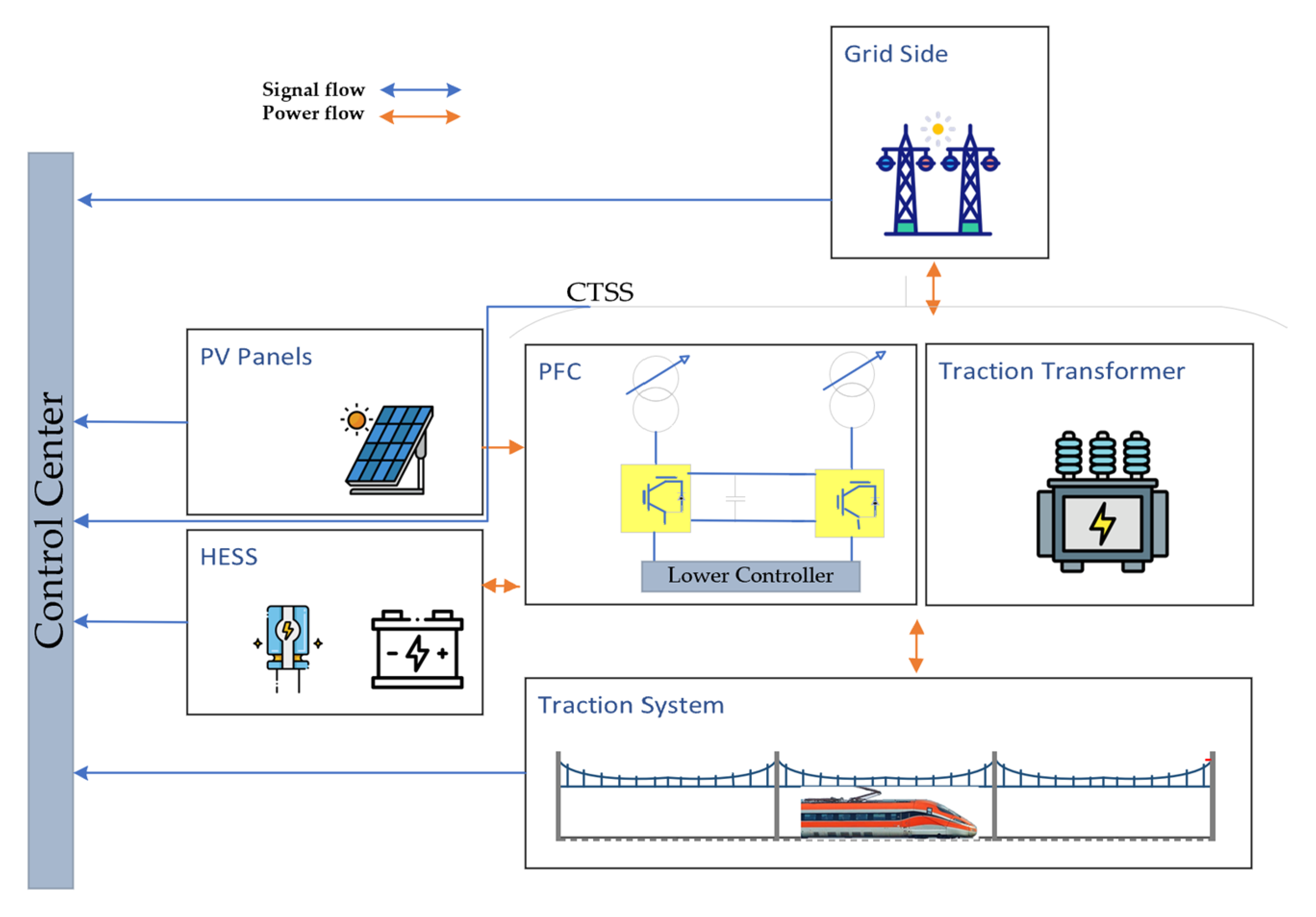
3. Architecture of the REM-S Network

Due to the dramatic increase in electricity usage from distributed resources in European railways [55], it is essential to update energy management methods consistently. In smart grid solutions (SGs), distributed energy management systems (EMSs) are commonly employed [56]. Several distributed systems, such as home energy management systems [57,58], smart city districts, and smart cities, are attempting to optimize energy scheduling. For instance, in reference [59], SGs are optimized to meet various load requirements and DERs, and reference [56] proposes a platform for smart buildings. In reference [56], the authors demonstrate the SG concept and its tools and framework can be applied to railway systems through the REM-S architecture.

The automation architecture implemented by REM-S is divided into two types: centralized and decentralized. It is possible to divide the railway system into local sections based on its specifications. Additionally, optimization targets can be defined locally or globally. A hybrid centralized–decentralized concept for REM-S was chosen based on these two major elements, together with other factors such as the degree of system complexity, the size of the system, and the structure and dependability of the different layers of the system. Hybrid centralized–decentralized REM-S architecture executes global EMS in a control center based on the entire railway network for the following day; at the same time, local EMS takes place in local subnetworks every 15 min.

A centralized–decentralized automation architecture can be designed using existing SG standards, communication protocols, and ICT technologies. Based on this, the railway distribution system is modelled as an SG in the architecture presented here [60]. Furthermore, it provides flexibility in terms of time horizons. The Smart Grid Architecture Model (SGAM) was initially created to assist in the standardization procedure for the SG, to possibly be applied to design SG architectures based on five types of interoperable layers (business, function, information, communication, and components), as well as zones and domains [61]. SGAM is illustrated through layers, zones, and domains in Figure 13.

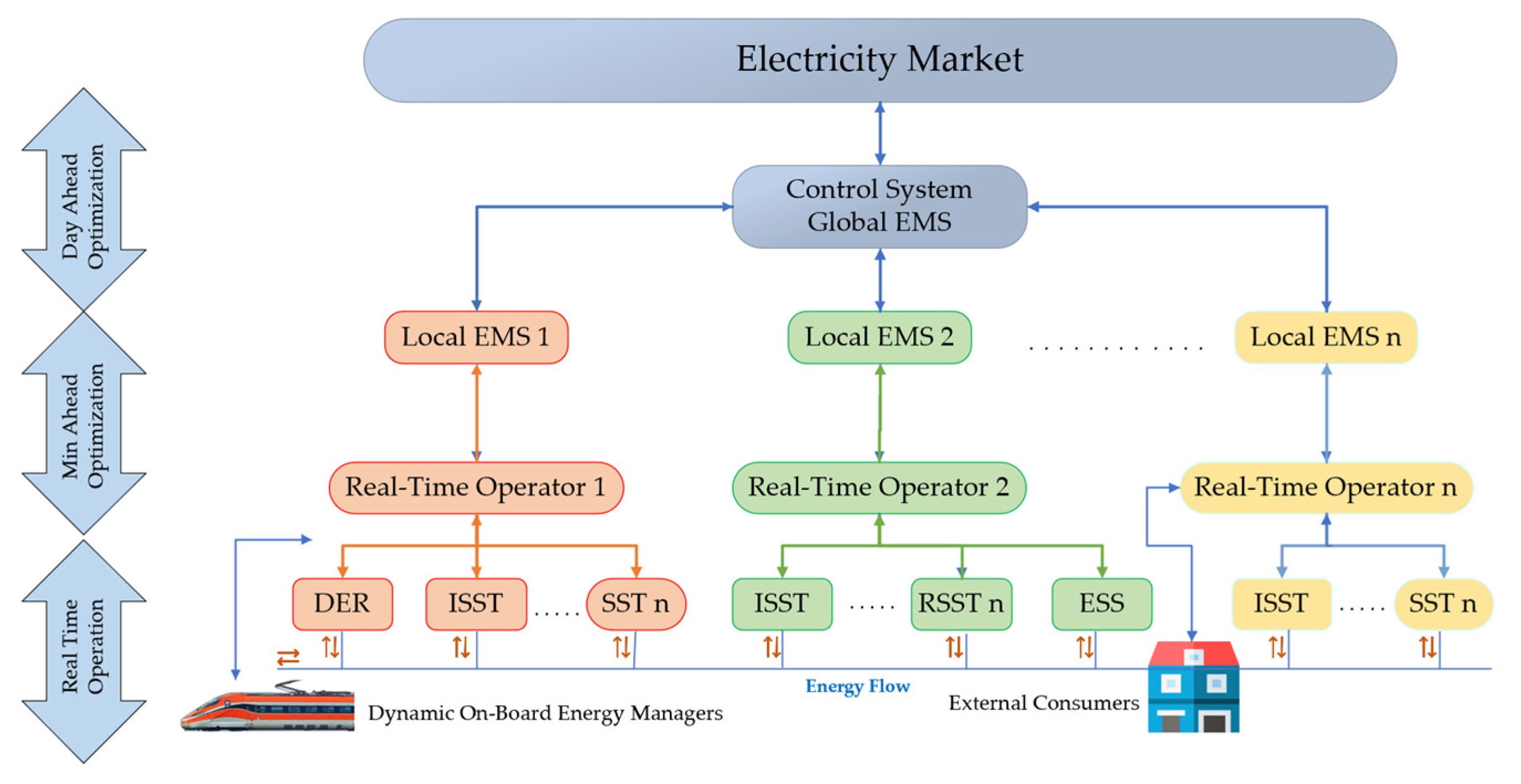
REM-S Automation Concept

Consumption optimization is one of the main purposes of REMS. The idea behind consumption optimization is to reduce electricity consumption on the public grid by regenerating or sparing energy by certain actors involved in the railway system and distributing it to other actors. Considering the large, complex, uncertain, and dynamic nature of railway loads, energy management must be based on subnetwork segmentation to address the distributed essence of the railroad system [56], and hybrid centralized–decentralized implementation is required.

By using an intelligent interface substation, each subnetwork is linked to the control center, which, in turn, connects it to the electricity market. Upon receiving the global optimization plan from the control center, subnetworks implement it locally in their own areas, and adjust for any unforeseen discrepancies. Regarding power and energy optimization in the border area, each subnetwork coordinates with neighboring subnetworks. Subnetwork automation and control are developed using multiagent systems (MAS) technology [62]. There is an intelligent entity for each energy-related component, called agent, which is capable of communicating with ISST, and is intelligent enough to decide whether to follow the directives or suggestions it receives.

Subnetworks consist of the following operational entities:

• intelligent substation (ISST): To send commands or suggestions to all elements associated with energy within the subnetwork, ISST is in communication with them. In every elements associated with energy, there is an intelligent entity, called an agent, that can communicate and make decisions in response to commands from ISST.
• Reversible Substations (RSST) and Nonreversible Substations (SST): Several of them negotiated with the main subnetwork agent to connect to the public grid as fixed agents.
• Wayside energy storage systems (ESSs): Assumed to be fixed agents.
• Distributed Energy Resources (DERs): Rail-related renewable resources situated within the subnetwork areas are also considered fixed agents.
• Dynamic On-Board Energy Managers (DOEMs) Installed on the Trains: Their responsibilities include energy management in trains along with contacting subnetworks ISST for recommendations. It traverses through subnetworks and maintains communication with each individual subnetwork’s main agent.
• External Consumers (ECs): In advanced multi-agent systems (MAS), fixed agents are established as workshops, stations, or other loads, such as electric vehicle (EV) charging stations.

It makes sense to adopt a similar time structure for optimization, yielding three approaches, given that the “railway system” interacts with the public grid and its market (electricity market) which is depicted in Figure 14.

• Day Ahead Optimization (DAO): Analyzes the performance of the network for the next day, and encompasses power profiles, energy and power procurement, as well as power sales, in the next 24 h.
• Minutes Ahead Optimization (MAO): Predicts and optimizes the subnetwork status for the next 15 min. In the same manner as the DAO profile, MAO interacts with all agents in the subnetwork, considering power limitations within the subnetwork, as well as excess supply and demand from neighboring subnetworks, the system proposes actions to subnetwork agents, such as SSTs, RSSTs, DERs, ESSs, or DOEMs, for the upcoming 15 min interval.
• Real-Time Operation (RTO): By leveraging the real-time status and behavior of all subnetwork elements, it successfully meets the calculated 15 min MAO profiles.

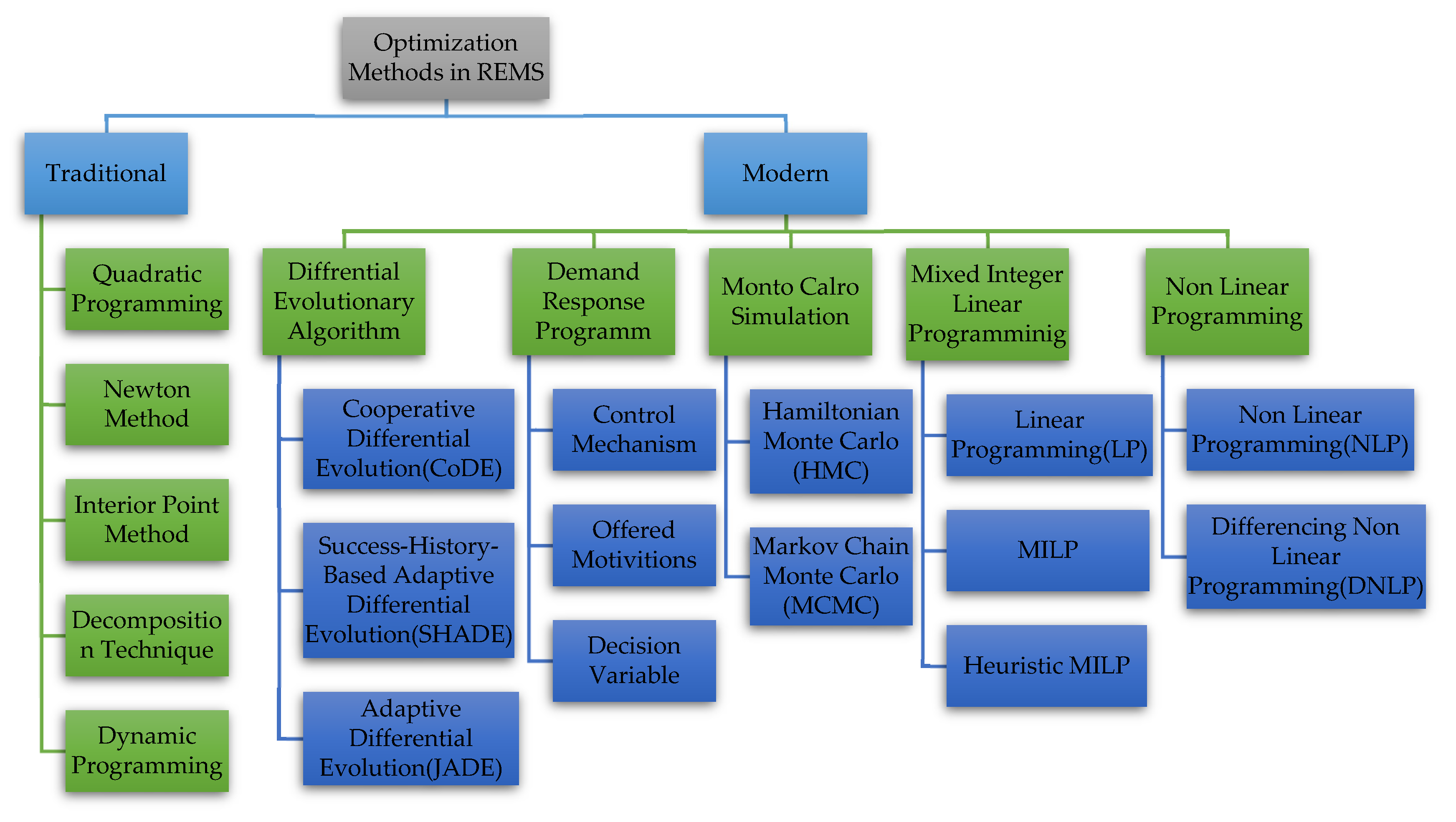
4. Optimization and Mathematical Methods

Power industry operations are strongly affected by the move to a competitive market. To run the system and control it efficiently, fast and robust optimization tools are more critical than ever. Optimization methods are widely used in power system analysis, planning, and operation. Optimized power flow (OPF) is an important application for dispatching engineers to handle large-scale power systems efficiently and effectively. Mathematical algorithms are utilized to solve global power system optimization problems so that the power system can be kept at the desired constraints. According to mathematic definitions, OPF is modelled as a nonlinear programming (NLP) problem whose output is usually minimized based on equality and inequality constraints applied to the expenses related to fuel consumption for thermal generating units and the deviation in voltage at the load bus [63].

As a computational problem, OPF represents a large-scale non-convex NLP with both nonlinear constraints and a nonlinear objective function. Discrete control parameters such as transformer taps and shunt capacitor banks transform the OPF problem into a mixed-integer NLP problem. The differential algorithm equations are also expressed if transient stability constraints are taken into account.

Some traditional optimization methods were used to solve the OPF problem in the past, including quadratic programming, Newton method, dynamic programming, decomposition technique, and interior point method, which are not used that much today. Nevertheless, they present some difficulties when it comes to handling non-linear, discrete-continuous functions and constraints. Additionally, traditional techniques have several disadvantages such as being time-consuming and containing more constraints in the mathematical formulation.

The application of evolutionary algorithms (EA) in various engineering fields is extensive [64,65,66,67], and they have proven to be particularly useful in electric railway systems [68]. Also, OPF problems have been solved using several modern stochastic algorithms to overcome these shortcomings. An evolutionary optimization technique that is commonly used is the Genetic Algorithm (GA) [69]. Similarly, it happens in Particle Swarm Optimization (PSO), which uses inertia weights, as well as social and cognitive parameters [70,71]. In the same way, Artificial Bee Colony (ABC) requires optimal controlling parameters of a limited number of bees (employed, scout, and onlookers) [72]. Harmonic Search (HS) takes into account the rate at which harmony memory is considered, the rate at which pitch is adjusted, and the number of improvisations [73].

In

Table 2. Optimization methods in REMS.

Traditional	Modern (Practical)
Quadratic Programming	Differential Evolution Algorithm
Newton Method	Demand Response Program
Dynamic Programming	Monte Carlo Simulation
Decomposition Technique	Mixed integer linear programming
Interior Point Method	Nonlinear Programming

, optimization methods are classified into two categories: traditional and modern (practical) methods. We will discuss a few of the traditional methods, and explain the modern methods in detail. Since the system in REMS is nonlinear and time-varying, we choose modern methods which are entirely used in Energy Management Systems for Smart Electric Railway Networks in the following subsections.

4.1. Traditional Optimization Methods

Quadratic Programming (QP) Methods can be classified as shared characteristics with linear and nonlinear programming algorithms. It is necessary to evaluate and compare a variety of QP algorithms to select the most promising method for solving Quadratic Reactive Power Dispatch (QRPD) [74]. In railway energy management systems, QP can be employed to optimize the distribution of energy resources, such as power allocation, based on predefined objectives and constraints. It helps find the optimal solution that minimizes energy consumption while satisfying operational requirements.

In Newton’s method, in every iteration, the Lagrangian function is solved by a direct simultaneous solution for all unknowns. The Lagrangian is approximated by a quadratic approximation each time it is iterated. It takes several iterations for any set of binding constraints to reach the Kuhn–Tucker conditions. The identification of binding inequalities is the hardest challenge in algorithm development [75]. Newton’s method is an iterative numerical technique used to find the roots of equations or optimize functions. In the context of railway energy management, Newton’s method can be applied to optimize energy-related parameters, such as train speed profiles, acceleration/deceleration patterns, and traction control systems. By iteratively refining these parameters, it aims to minimize energy usage while maintaining operational requirements.

Mathematically optimal solutions are generated by dynamic programming. Furthermore, dynamic programming aligns sequences that are not related. Statistics also require clever theory to determine when a score is statistically significant [76]. An economic dispatch problem can be solved mathematically using a Decomposition Technique. Several subproblems concerning specific power system areas are decomposed from the system’s optimization problem [77]. In some optimal power flow applications, the interior point method was found to be very effective due to the primal-dual algorithm and the numerical results for large-scale networks (1832 and 3467 bus systems) in the past [78].

4.2. Modern (Practical) Optimization Methods

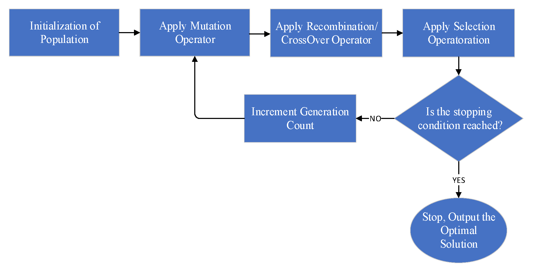
4.2.1. Modified Differential Evolution Optimization Algorithm

Differential evolution (DE) is a stochastic direct search optimization method and it was presented as a heuristic optimization method [79]. With differential evolution, a special differentiation operator encodes the evolution algorithm in a floating point for global optimization. By employing this operator, independent offspring were created instead of classical crossovers or mutations [79,80,81,82,83,84].

DE solves real-valued problems using a population ‘P’ of population size ‘NP’ floating point-encoded individuals where the individuals are D-dimensional variable vectors that evolve over ‘G’ generations to reach an optimal solution [63], which means:

$$P=\left[x_1\right(G),\dots \dots \dots \dots \dots ,x_{NP}(G\left)\right]$$

(1)

$$x_i\left(G\right)=\left[x_{1i}\right(G),x_{2i}(G\dots \dots \dots ,x_{Di}\left(G\right)] i\dots ,2,\dots \dots ,NP$$

(2)

It is recommended to uniformly randomize individuals within the defined minimum and maximum parameters as constraints in order to better cover the entire search space by the initial population.

$$x_j^{\min }=\{x_1^{\min },\dots \dots \dots ,x_D^{\min }\} \mathrm{and} x_j^{\max }=\{x_1^{\max },\dots \dots \dots ,x_D^{\max }\}$$

(3)

During optimization, mutations, crossovers, and selections are carried out. It is also necessary to tune a number of optimization parameters. They are commonly referred to as control parameters. Essentially, there are only three main parameters in the algorithm, which are the mutation constant ‘F’, crossover rate ‘CR’, and population size ‘NP’. There are two other parameters, the dimension of problem ‘D’, which scales the difficulty of the optimization task; the number of generations (or iterations) ‘G’, which can act as a stopping condition; and the lower ($x_j^L$) and upper ($x_j^U$) bounds of the $j_{}^{th}$ decision parameter, which limit the possible areas [63].

The Computational Flow of DE

As shown in Figure 15 [35], DE follows a simple cycle of stages. These stages can be accomplished as follows:

• Step 1: Initialization

Problem-independent variables are initialized in their feasible ranges at the beginning of a DE run. In other words, if the jth variable of the given problem has its lower and upper bounds as $x_j^L$ and $x_j^U$, respectively, then initializing the jth component of the ith population may be carried out as follows:

$$x_{i,j}\left(0\right)=x_j^L+rand(0,1).(x_j^U-x_j^L)$$

(4)

Each value of j generates a random number between 0 and 1 that is uniformly distributed between 0 and 1.

• Step 2: Mutation

Evolution is carried out through mutation, crossover, and selection operators after the population is initialized. Different strategies are employed for crossover and mutation. How the scheme works in its simplest form is explained here in detail. Introducing new parameters into the population is the responsibility of the mutation operator. Equation (5) explains the process of the mutation operator, which generates mutant vectors by modifying a vector ($x_{i1}$) chosen randomly using the difference between two other randomly selected vectors ($x_{i2}$ and $x_{i3}$).

This condition requires at least four individuals to satisfy since all these vectors must be different. A user-defined constant (F) is applied to the difference vector in the range of 0.4–1.0 to control the perturbation and improve convergence. The scaling constant is also known as a differentiation (or mutation) constant. $x_i\left(G\right)$ (i = 1, 2, ……, NP) of generation G (G = 1, 2, …, G), of the population is changed by mutating the target vector. When a population member, $x_i\left(G\right)$ of generation G is changed, a trial vector, $V_i(G+1)$ is created by mutating a target vector [84].

DE schemes are differentiated by the method used to create these donor vectors. An $i_{th}$ member’s trial vector $V_i(G+1)$ is created based on three-parameter vectors $x_1$, $x_2$, and $x_3$, selected randomly from the current population but not matching $x_i$. Once the trial vector $V_i(G+1)$ is obtained, a scalar number F is used to scale the difference between any two of the three vectors. In most cases, F is between 0.4 and 1.0. In other words, for each vector, the $j^{th}$ component is expressed as follows:

$$V_{i,j}(G+1)=x_{i1,j}\left(G\right)+F.\left[x_{i2,j}\right(G)-x_{i3,j}(G\left)\right]$$

(5)

• Step 3: Crossover

Crossover operators increase the diversity of the population by exchanging parts of the donor vector with those of the current member $x_{i,j}\left(G\right).$ No crossover is performed when a randomly picked number goes beyond the first CR value and the remaining variables remain unchanged. The literature offers two types of crossover operators: binomial crossover and exponential crossover. As a result of binominal crossover, the generated child $U_{i,j}\left(G\right)$ is [84]:

$$x_{i,j}(G+1)=x_{i,j}\left(G\right) \mathrm{if} ran{d}_{j,i}\le CR$$

(6)

$$U_{i,j}\left(G\right)=x_{i,j}\left(G\right) \mathrm{if} ran{d}_{j,i}>CR$$

(7)

In this case, CR is the crossover rate, whereas $U_{i,j}\left(G\right)$ is the child that will compete against the parent $x_{i,j}\left(G\right)$.

• Step 4: Selection

Comparing the trial individual $U_{i,j}(G+1)$ with the corresponding $V_{i,j}(G+1)$ determines whether it should enter the next generation. During the selection process, the trial individual is assessed against the corresponding one on the basis of fitness survival:

$$x_{i,j}(G+1)=U_{i,j}(G+1) \mathrm{if} U_{i,j}(G+1)\le x_{i,j}\left(G\right)$$

(8)

$$x_{i,j}(G+1)=x_{i,j}\left(G\right) \mathrm{otherwise}$$

(9)

Ref. [47] utilizes the Differential Evolution Optimization Algorithm in Electrical Railway Systems.

4.2.2. Demand Response Program

There are a number of Demand Side Management (DSM) activities, including Demand Response (DR), which is considered a subset of the broader category of DSM [85,86,87]. According to the US Department of Energy, DR is a tariff or program intended to motivate customers to reduce their electric consumption based on changes in the cost of electricity. It is also intended to provide incentive payments intended to reduce electricity consumption at times of high market prices or in times of impaired grid reliability [88].

According to this definition, DR should be appealing to consumers. In this way, they can manage their power consumption preferences so that consumers and the power grid will benefit [89]. It also improves the efficiency and reliability of the power grid by allowing power demand to be adapted to time pricing or incentives [90,91]. It is crucial to design an efficient DR program in order to deploy a smart grid [92].

There are three categories of DR schemes, as illustrated in Figure 16 [93]. DR schemes are classified into centralized and distributed in the first category based on the control mechanism. During the distribution mode, utility information is collected from interactions between users, while in the centralized mode, consumers communicate directly with the utility [94].

According to their motivations for reducing power consumption, DR schemes are classified into the second category [95]. Generally, these motivations can be classified as time-based DR and incentive-based DR. Time-based DR (also known as price-based DR [96]) engages consumers in time-varying payments based on the price of electricity at different times. Meanwhile, incentive-based DR schemes offer fixed or variable payments to customers to motivate them to reduce their electricity consumption during times of stress [97], but customers are also subject to specific restrictions or penalized for not participating.

As a final category, task-scheduling DR schemes (also known as energy or power scheduling DR schemes) employ the decision variable to identify DR schemes [98]. The key function of task scheduling DR is to control the activation time of requested loads, which can be moved to peak periods [99]. It is possible to reduce power consumption during peak-demand hours by using energy management-based DR schemes [98].

It is not enough to just implement DRP in Energy Management for Smart Railways. As ref. [48] mentions, in order to enhance the adaptability of the energy hub system (EHS), DRP is integrated into the model. Afterwards, a fuzzy technique can be employed to choose the best solution.

4.2.3. Monte Carlo Simulation

In a process where random variables interfere, Monte Carlo simulation is used to model the probability of different outcomes. Uncertainty and risk are understood using this technique. A variety of problems can be solved using a Monte Carlo simulation, including in the fields of investing, business, physics, and engineering. It is also known as a multiple probability simulation. Forecasting or estimating with significant uncertainty can use an average instead of an uncertain variable. Instead, Monte Carlo Simulation uses multiple values and averages them.

Monte Carlo acknowledges a problem for any simulation method: random variables interfere with pinpointing the probability of varying outcomes. As a result, Monte Carlo simulations focus on repeatedly taking random samples. The Monte Carlo simulation assigns a random value to the variable that is under uncertainty. This is followed by running the model and providing a result. As the variable is assigned many different values, this process is repeated numerous times. Estimates are obtained by averaging the results after the simulation is complete [100].

Random Number Generators Based on Linear Recurrences

The core of all Monte Carlo methods requires a uniform random number generator, which generates an infinite stream of random numbers U1, U2, … in the interval (0, 1). The prevalent approach for generating uniformly distributed random numbers is to use recurrence relations based on simple linear equations [101]. Linear congruent generators (LCGs) produce output streams with the form $U_t=X_t/m$, where $X_t$ is a linear recurrence state:

$$X_t=(a{X}_{t-1}+c) \mathrm{mod} \mathrm{m},\mathrm{t} = 1, 2, \dots$$

(10)

A modulus, multiplier, and increment are defined as m, a, and c, respectively. Applying the modulo-m operator in Equation (1) means that $a{X}_{t-1}+c$ is divided by m, and the remainder is taken as the value for $X_t$.

Multi-recursive generators (MRG) of order k produce defined by a k-dimensional vector $X_t=(X_{t-k+1}+\dots +X_t{)}^T$ that satisfies the linear recurrence rule of $X_t$:

$$X_t=(a_1{X}_{t-1}+\dots +a_k{X}_{t-k}) \mathrm{mod} \mathrm{m},\mathrm{t} = \mathrm{k}, \mathrm{k}+1, \dots$$

(11)

In the case of some moduli and multipliers I = 1, …, k.

Almost all multipliers should be zero in order to produce fast algorithms. As in the LCG case, when m is a large integer, $U_t=X_t/m$ yields a stream of random numbers. Additionally, m = 2 makes the generator state represented by a binary vector of length k. This produces the following output function:

$$U_t={\sum }_{i=1}^w{X}_{tw+i-1}{2}^{-i}$$

(12)

For some w < k, for instance, w = 32 or 64. There are various modulo 2 generators, most notably Mersenne twisters, which use feedback shift registers [102,103]. It is possible to combine several simpler MRGs to produce MRGs with excellent statistical properties [104].

• Generating Random Variables: Inverse–Transform Method

Assume X is a random variable with a cumulative distribution function (cdf). Then $F^{-1}$ represents the inverse of F and U represents the uniform random number (0, 1), which means U ∼ U(0, 1). Therefore:

$$P\left(F^{-1}\right(U)\le x)=P(U\le F(x\left)\right)=F\left(x\right)$$

(13)

An inverse–transform method is employed to generate a random variable X using cdf F: draw U ∼ U(0, 1) and return X = $F^{-1}$ (U).

➢

Generating Random Variables: Acceptance–Rejection Method

• Generate X ∼ g; that is, draw X from pdf g.
• Generate U ∼ U(0, 1), independently of X.
• If $U\le f\left(x\right)/\left(Cg\right(x\left)\right)$ output X; otherwise return to step 1.

1/C is the probability of acceptance in the acceptance–rejection method. The acceptance–rejection method can also be used to generate random vectors in X ∈ $R^d$.

2.

Generating a Markov Chain

• Draw $X_0$ from its distribution. Set t = 0.
• Draw $X_t+1$ from the conditional distribution of the $X_t+1$ given $X_t$.
• Set t = t + 1 and repeat from Step 2.

As a result, the conditional distribution of $\left(X_{t+s}|X_t\right)$ is time-homogeneous in a vast majority of cases of relevance. There are various types of diffusion processes, all of which satisfy the Markov property and are random processes with continuous paths and continuously varying time parameters.

➢

Markov Chain Monte Carlo

The Markov Chain Monte Carlo (MCMC) method is a general method for sampling from any type of distribution. In this technique, we generate a Markov Chain whose limiting distribution is the desired distribution.

Referring to reference [105], the MCMC method can be applied to the following settings. In the case of arbitrary multidimensional PDFs, let us attempt the following:

$$f(x)=\frac{p\left(x\right)}{Z} , x\in X$$

(14)

A positive function p(x) is represented by a known or unknown normalizing constant Z. Considering $q\left(y\right|x)$) as an instrumental density or proposal, describes how to move from state x to state y using a Markov transition density.

Monte Carlo for Optimization: Stochastic Approximation

• Initialize $x_1$ ∈ X. Set t = 1.
• Obtain an estimated gradient ∇S($x_t$) of S at $x_t$.
• Determine a step size ${\beta }_t$.
• Set $x_{t+1}={\Pi }_x\left(x_t-{\beta }_t\nabla S\left(x_t\right)\right).$

If a stopping criterion is met, stop; otherwise, set t = t + 1 and repeat from Step 2.

In stochastic approximation algorithms, many theorems exist about convergence. Specifically, for arbitrary deterministic positive sequences β1, β2, … such that:

$${\sum }_{t=1}^{\infty }{\beta }_t=\infty , {\sum }_{t=1}^{\infty }{{\beta }^2}_t<\infty$$

(15)

A random sequence $x_1,x_2$, converges to the minimizer $x^{*}$ of S(x) in the mean square sense if there are certain regularity conditions [106]. If $\nabla S\left(x_t\right)$ is an unbiased estimator of $\nabla S\left(x_t\right)$ in $x_{t+1}={\Pi }_x(x_t-{\beta }_t\nabla S(x_t\left)\right)$, an algorithm for stochastic approximation is known as the Robbins–Monro algorithm.

An algorithm called the Kiefer–Wolfowitz algorithm is used to estimate $\nabla S\left(x_t\right)$ using finite differences. Stochastic counterparts (also called sample average approximations) are an alternative approach to stochastic approximation if:

$$\underset{x\in R^n}{min}S(x)$$

(16)

where

$$S(x)=\frac{1}{N}{\sum }_{i=1}^{N}S(x,{\xi }_i)$$

(17)

is a sample average estimator of $S(x)=ES(x,{\xi }_{})$ on the basis of N samples ${\xi }_1$,…,${\xi }_N$. An estimate of the solution $x^{*}$ to the original problem $\underset{x\in X}{min}S\left(x\right),$ is taken as a solution $x^{*}$ to this sample average version. It should be noted that $\underset{x\in R^n}{min}S\left(x\right)$ is a deterministic optimization problem that can be solved with any of the standard deterministic optimization methods. The authors of refs. [42,44] applied this method in order to implement their electrical railway model.

4.2.4. Mixed Integer Linear Programming

➢

LP Computability

While Quadratic Programming (QP) models are relatively straightforward in solving the problems, Linear Programming (LP) models are generally considered more computationally practical. The software designed specifically for solving Linear programming (LP) models exhibit a higher level of sophistication when compared to quadratic programming (QP) models. As a result, there are numerous commercial LP solvers available, and they are generally considered to be more reliable than QP solvers. In general, LP solvers are capable of finding solutions within a short time frame, typically in seconds, whereas QP solvers may require more time [107].

A scenario refers to a potential situation that could occur at the specified time. Specifically, it represents a plausible outcome of asset returns at the designated time. Taking into account events and circumstances between the investment period and the target time, various alternative scenarios may unfold. Scenarios have different probabilities and may be more or less likely to happen. Here, the basis of an accurate preliminary analysis is assumed. We consider T different scenarios $S_t$, t = 1, …, T, that are possible at the target time.

The probability scenario t will happen in time represented as $P_t$ and has the following cumulative relation:

$${\sum }_{t=1}^T{P}_t=1$$

(18)

For each random variable $R_J$, J = 1…, n, its realization $r_{Jt}$ under scenario t exists and is known. Indeed, a scenario is defined by the set of return of all assets ($r_{Jt}$). In the same way, the correlation among the rates of return of the assets are captured by the concept of scenario.

The expected return of asset j is calculated as Equation (19):

$${\mu }_J={\sum }_{t=1}^T{P}_t.r_{Jt}$$

(19)

Determining the scenarios and their probabilities and calculating the values of the rate of return $r_{Jt}$ of each asset j under each scenario t is essential. One of the most vital notes that we have to consider while solving an LP is that the number of scenarios has to be sufficiently large, until the statistical conditions are satisfied.

Each portfolio x represents a corresponding random variable $R_x$ which characterizes the portfolio rate of return and can be obtained by following equation:

$$R_x={\sum }_{J=1}^n{R}_J.X_J$$

(20)

The step-wise cumulative distribution function (cdf) of $R_x$ is defined as:

$$F_x\left(\xi \right)=P(R_X\le \xi )$$

(21)

is the return of a portfolio x in scenario t that is computed as Equation (22). This parameter is a kind of efficiency.

$$y_t={\sum }_{i=1}^n{r}_{Jt}.x_J$$

(22)

Equation x indicates the expected return of the portfolio ${\mu }_x$ as a linear function of (23).

$${\mu }_x=E\{R_x\}={\displaystyle \sum _{t=1}^T{P}_t}.y_t={\displaystyle \sum _{t=1}^T{P}_t}({\displaystyle \sum _{J=1}^n{r}_{Jt}.}{x}_J)={\displaystyle \sum _{J=1}^n}{x}_J{\displaystyle \sum _{t=1}^T{P}_t}{r}_{Jt}={\displaystyle \sum _{J=1}^n{\mu }_J.}{x}_J$$

(23)

In the given context, the scenario can be described as an instance of a multivariate random variable that represents the rates of return of various assets. We can view the set of scenarios as a discretization of this multivariate random variable. When the returns are observed and quantized according to the specified scenarios, they become discretized.

It is important to highlight that a risk or safety measure can be computed using Linear Programming (LP) if the portfolio optimization model adopts a linear structure when applied to discretized returns. By using Equation (24), risk measures $\partial \left(x\right)$ can be defined as:

$$\partial (x)=\min \{a_{}^{T}v:Av=Bx,v>0,x\in Q\}$$

(24)

In this formula, v is a vector of auxiliary variables, and x is the portfolio vector. b = Bx is the parametric right-hand side vector.

The corresponding safety measures are determined using a comparable LP formula as follows:

$$\mu (x)-\partial (x)=\mathit{max}\{{\sum }_{J=1}^n{\mu }_J.x_J-a^{T}v:Av=Bx,v>0,x\in Q$$

(25)

➢

MILP Computability

Linear Programming (LP) stands as one of the fundamental optimization techniques extensively employed in various practical applications. The advantage of LP over alternative methods lies in the existence of proficient software packages capable of effectively solving large-scale problem instances. When formulating an LP problem, the software diligently explores the solution space to identify the optimal solution. However, in cases where the problem formulation necessitates the presence of inherently integer or binary variables, the LP problem transforms into a Mixed-Integer Linear Programming (MILP) model.

When dealing with large Mixed-Integer Linear Programming (MILP) problems, heuristics become indispensable. The extensive literature offers a wide range of heuristic and metaheuristic approaches to choose from. For a specific problem, a tailored heuristic inspired by these schemes can be designed and implemented. Numerous research papers have been dedicated to developing problem-specific heuristics. However, this approach can pose challenges for portfolio optimization due to the necessary expertise and resource-intensive nature of designing and implementing problem-specific heuristics. Even minor variations in the problem may necessitate re-designing the heuristic, incurring additional time and cost.

To address these challenges, general-purpose methods offer advantages as they can be applied to a broad class of MILP problems. An optimal, versatile heuristic should possess efficiency, enabling it to effectively tackle extensive MILP problems within a reasonable timeframe, and effective, providing solutions close to optimality. The desire for heuristics that are both efficient and effective, along with the availability of software able to efficiently process small MILP problems, has given rise to the emergence of matheuristics methods. Matheuristics combine heuristic strategies with the solution of small MILP subproblems, leveraging existing software for the latter.

In this context, we introduce Kernel Search, a flexible and versatile matheuristic method that requires minimal implementation effort. It offers a general approach that can be applied to a wide range of MILP problems, making it a valuable tool for optimization tasks.

Mixed Integer Linear Programming (MILP) represents a potent mathematical programming approach employed to optimize intricate linear systems. In MILP models, the objective function is optimized by adjusting the values of decision variables while adhering to specific constraints that govern the permissible values of these variables. This approach enables the identification of optimal solutions that balance the objectives of the problem with the given constraints, thereby aiding in the efficient resolution of complex optimization challenges.

A mixed integer linear program (MILP, MIP) is of the form:

$$\begin{gathered} \min C^T.x \\ Ax=b \\ x>0 \\ {x}_i\in Z\hspace{1em}\forall i\in Z \end{gathered}$$

(26)

If all variables need to be an integer, t is called a (pure) integer linear program (ILP, IP). If all variables need to be 0 or 1 (Binary, Boolean), it is called a 0–1 linear program.

Including integer variables increases the modeling power enormously, at the expense of more complexity. LPs can be solved in polynomial time with interior-point methods (ellipsoid method, Karmarkar’s algorithm). Integer Programming is an NP-hard problem, so:

• There is no known polynomial–time algorithm.
• There are little chances that one will ever be found.
• Even small problems may be hard to solve.

➢

Heuristic MILP

This section introduces the Kernel Search, a versatile metaheuristic that can be employed for a wide range of MILP problems and their variations. The proposed approach is suitable for minimizing MILP problems and encompasses multiple sets of variables. To illustrate the performance of the Kernel Search, a basic variant called Basic Kernel Search (BKS) is presented. BKS serves as a foundational version that demonstrates the core principles and effectiveness of the Kernel Search metaheuristic.

The BKS (Basic Kernel Search) approach involves solving a sequence of constrained problems. In this sequence, the complete set of assets is denoted as N = {1, …, n}. The MILP(K) formulation is employed to represent the MILP problem that is constrained to a specific subset of assets, denoted as K ⊆ N. The aim of the BKS is to determine the assets that would be part of an optimal solution for the original problem and then solve the MILP problem using only those chosen assets. By iteratively applying this process, the BKS aims to find an effective solution by progressively refining the set of assets considered in the MILP problem.

In the majority of optimization problems, the number of assets that are relevant or active is relatively small, typically less than 100. Consequently, although solving the MILP problem with the entire set of assets may be computationally demanding, the MILP problem involving a subset of a hundred assets can generally be solved within a reasonably short computational time. This observation allows for more efficient optimization by focusing on the essential assets and significantly reducing the computational burden.

The BKS (Basic Kernel Search) algorithm aims to identify a subset of assets, known as the kernel, that are prone to being selected in an optimal solution for the original problem. Any assets not included in the kernel are placed into buckets. The assets are then sorted based on their likelihood of contributing to an optimal portfolio. The initial kernel is formed by selecting the first n_I assets in this sorted order.

After categorizing the remaining assets into distinct groups or buckets, the BKS algorithm solves the MILP problem with the assets confined to the initial kernel. Next, the algorithm iteratively revises the kernel by solving the MILP problem which is constrained to the specific assets that have been selected in each individual bucket. This iterative process continues until all buckets have been processed, resulting in the refinement of the kernel. BKS is provided in the following algorithm:

• Determine the initial kernel and arrange the remaining assets into a sorted collection of buckets.
• Find the solution to the MILP problem by considering only the assets within the initial kernel.
• Continue the process repeatedly until a specific condition or criterion is satisfied:
  • Modify or update the kernel;
  • Find the solution to the MILP problem by considering the assets within the current kernel along with the assets in the next bucket on the list;
  • Exclude or eliminate the bucket from the list.

References [40,44,51,52] implement this method in their papers.

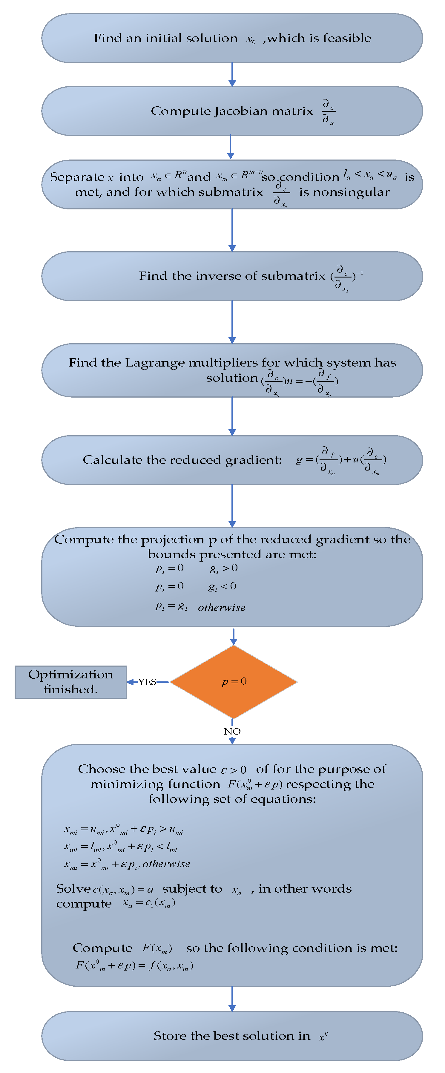
4.2.5. Non-Linear Programming

The GAMS (Generalized Algebraic Modeling System) optimizer software package is widely used in industrial applications and academic research in applied sciences and mathematics. Among the most notable capabilities of GAMS for the solution of mathematical optimization models is its ability to solve linear as well as nonlinear models and to include continuous, discrete, and binary variables [108]. There are six basic components of the mathematics model coded in GAMS: sets, data, variables, equation, model, and output. There are many solvers in GAMS that deal with models of mathematical programming such as deterministic global optimization, stochastic programming, linear programming, linear regression, and others.

However, it is necessary to use a nonlinear programming (NLP) algorithm when solving nonlinear models created with GAMS. In GAMS, there are two types of nonlinear models: nonlinear programming (NLP) and differencing nonlinear programming (DNLP). The NLP pattern is a smooth function with smooth derivatives that appears in model variables that have endogenous arguments. A DNLP model can also use functions that have smooth derivatives but discontinuous ends. Therefore, NLP models are usually used. There are a large number of various solvers for solving NLP in GAMS, and CONOPT solver is one of the fastest solvers.

It is possible to formulate the CONOPT optimization algorithm in the following way [109,110]:

$$\mathit{min}{\sum }_{i=1}^E{x}_{ji}$$

(27)

Subject to:

$$c_i(x_i,x_{i-1},\dots ,x_{i-t})=b_i i=1,\dots ,E$$

(28)

$$l_i\le x_i\le u_i i=1,\dots ,E$$

(29)

A vector $x_i$ represents the optimization variables in period i, a vector $c_i$ represents constraint values in period i, a vector $b_i$ represents the right-hand sides in period i, a vector $l_i$ represents the lower bounds in period i, a vector $u_i$ represents the upper bounds in period i, a vector $x_{ji}$ represents the $j^{th}$ component of vector $x_i$, and a time horizon indicates the end point. Figure 17 shows the flow chart for the CONOPT algorithm [108]. Also, ref. [48] uses NLP in order to achieve modeling.

In the preceding sections, a comprehensive overview of both modern and traditional methods employed in railway energy management systems has been presented. These methods play a crucial role in optimizing energy consumption and enhancing the efficiency of railway operations. To further illustrate the breadth of these approaches, a chart showcasing the various methods and their respective variants is provided in Figure 18. Furthermore, the most common general purposes for the methods application together with their main references are provided in

Table 3. Different methods used in ERS.

Methods Type	Method Name	General Purpose and References
Traditional	QP	Classified shared characteristics with linear and nonlinear programming algorithms [74]. Global minimization of the inequality constraints problems [111]. Analysis application of a new recurrent neural network for quadratic programming [112].
	Newton	Solve the Lagrangian function by a direct simultaneous solution for all unknowns [75]. Calculating wear between two elastic bodies in contact [113]. Solve a set of n nonlinear simultaneous equations, and obtaining a correction to each element of the approximate solution [114].
	IPM	Primal-dual algorithm and the numerical results for large-scale networks [78]. Solve the optimal control problem in model predictive control [115]. Solve the general nonlinearly inequality constrained problems [116].
	DT	Solve the economic dispatch problem [77]. Coordinating the mid and short-term scheduling of hydrothermal systems [117]. Identify and quantify the separate contributions of group differences in measurable characteristics [118].
	DP	Optimize solutions to align sequences that are not related [76]. Optimizing the train running profile [119]. Application to discrete-utterance and connected-speech recognition [120].
Modern	DEA	Optimal energy management of railroad electrical systems [45]. Examines the problem of scheduling railway timetables [121]. Fuel loading optimization [122].
	DRP	Prime operation of a smart railway station [48]. Measuring consumer response to static time-of-day and seasonal prices [123]. Reduce consumers’ load in real-time once the prices goes beyond a specific point [124].
	MCS	Optimum operation of smart railway stations [49]. Minimizing the operational cost in REMS [47]. Evaluation of kinetic parameters and their effect on the biomass pyrolysis [125].
	MILP	Energy management for railway substation [51]. Robust energy management of high-speed railway [52]. Minimizing the operational cost of smart railway station [44].
	NLP	Ultimate AC power flow for ERSs’ operation [21]. An optimal operation strategy for an ERS’s station based on combined cooling, heating, and power systems [126]. An optimal AC power flow problem for ERSs’ operation [46].

. This visual representation offers a concise reference for readers, facilitating a deeper understanding of the diverse strategies utilized in railway energy management.

5. Discussion

As discussed in the previous section, in the context of electric railway systems, various methods can be applied for the energy management and optimization of systems. These methods are classified into two main categories of traditional and modern methods. In summary, traditional methods are well-established and computationally efficient for handling linear or quadratic problems but may have limitations when dealing with nonlinear or non-convex optimization problems, especially for non-linear and complex systems such as ERS. On the other hand, modern methods offer more flexibility, improved global optimization guarantees, and the ability to handle complex, nonlinear, or discrete problems. However, they may require more computational resources and could have slower convergence compared to traditional methods. The choice of method depends on the specific problem characteristics, available computational resources, and the trade-off between solution quality and computational efficiency. Accordingly, in this paper we mostly concentrated on modern methods.

NLP finds applications in optimizing power flow, energy management, and scheduling tasks in the railway domain. It can be used to control the distribution of power, manage energy resources efficiently, schedule electric vehicle charging stations, and optimize train timetables while considering energy efficiency and operational constraints.

DEA is useful for fine-tuning parameters and optimizing control strategies in traction systems, optimizing maintenance schedules for railway infrastructure, and allocating resources efficiently for energy management. DEA can also aid in optimizing the usage of battery storage and regenerative braking systems.

MCS plays a valuable role in analyzing uncertainties and assessing the risks associated with energy consumption and demand forecasting. It helps evaluate the reliability of power supply and distribution networks and assesses the impact of random events on system performance and energy efficiency.

MILP finds application in various tasks within railway systems. It can optimize the design and allocation of substations and power distribution infrastructures, facilitating energy-efficient train scheduling and routing considering capacity constraints and energy regeneration, and enabling the multi-objective optimization of railway systems by incorporating factors like energy consumption, travel time, and passenger satisfaction.

In summary, NLP, DEA, MCS, and MILP each offer technical capabilities for different aspects of energy management in railways, ranging from optimal control and scheduling to parameter tuning, uncertainty analysis, and infrastructure optimization. These applications highlight the diverse suitability of each method depending on the specific requirements and characteristics of the electric railway system being studied. By carefully assessing the problem, constraints, and objectives, researchers and practitioners can determine the most appropriate method or combination of methods for a given energy management application in electric railway systems.

The above-mentioned research allows us to compare all modern methods used in REMS. Comparing optimization techniques quantitatively can be challenging because their performance depends on various factors such as problem complexity, data availability, solver efficiency, and specific problem constraints.

Table 4. Different methods comparison.

Technique	Speed	Simplicity	Efficiency	Robustness	Accuracy	Performance
NLP	Varies based on problem complexity and solver efficiency	Moderate complexity due to nonlinear nature	Can handle large-scale problems efficiently with suitable solvers	Sensitive to problem formulation and initial conditions	Highly dependent on problem formulation and solution approach	Can provide high-quality solutions, but convergence may not always be guaranteed
DEA	Fast and efficient	Relatively simple	Can handle large datasets efficiently	Robust against outliers and noise in the data	Based on relative efficiency rather than absolute accuracy	Provides comparative efficiency scores and rankings
MCS	Moderate speed	Relatively simple	Computationally demanding for a large number of iterations	Robust in capturing uncertainty and variability	Accuracy depends on the quality of probability distributions used	Provides probabilistic outputs and risk analysis results
MILP	Varies based on problem complexity and solver efficiency	Moderate complexity due to integer variables	Can handle large-scale problems with efficient solvers	Robust against problem formulation and constraints	High accuracy in finding optimal or near-optimal solutions	Provides optimal solutions and guarantees optimality under certain conditions

presents a general comparison of all modern methods for a greater ease of understanding. This table generally compares the performance of the methods. However, their suitability and performance in this specific context may vary depending on the nature of the energy management problem, the availability of data, the specific constraints and objectives involved, and the underlying modeling assumptions. It is essential to assess the requirements and constraints of your energy management system to determine the most suitable optimization technique for your specific needs.

As mentioned, DEA is a stochastic direct search optimization, and because of its simplicity and high speed, this method has a good efficiency. However, DEA only solves real-valued problems and there are many constraints associated with this method.

NLP and DNLP are two varieties of nonlinear programs. One of the main advantages of DNLP is the ability to use functions with smooth derivatives and discontinuous ends. Compared to linear methods, NLP offers higher accuracy but also more complexity. In support of this, in ref. [46], the author considered the same system and used DEA and NLP methods and compared them from an efficiency point of view; as a result, the total operation cost saving was higher in NLP than in DEA.

MCS require a uniform random number generator which generates an infinite stream of a random number in the interval (0, 1), which is a disadvantage of this method; in addition, we have to use a reduction technique to reduce the variables. As MCS focus on repeatedly taking random samples, for a large number of variables, it requires a lot of time and computations; as a result, this method is not fast.

DRP has a featured disadvantage in that the DRP model is not enough to only be implemented in REMS, and it has to integrate into a model; thus, it is not very efficient.

In a Mixed Integer Linear Program, variables are integers which can be pure integer linear programs or they are 0 and 1—the so-called binary linear program—and both are stochastic. MILP does not consider decimal variables, which is not an advantage of this model. Figure 19 shows a comparison of the main methods used in REMS from different performance points of view.

Overall, modern methods such as DE, DRP, MCS, MILP, and NLP offer more advanced capabilities to handle complex and nonlinear optimization problems in railway energy management systems. They often provide greater flexibility, improved global optimization guarantees, and the ability to handle discrete variables or dynamic scenarios. However, the choice of method depends on the specific problem characteristics, available computational resources, and the trade-off between solution quality and computational efficiency.

6. Conclusions

This review paper has provided a comprehensive examination of railway energy management systems (REMS). The focus was on exploring the various architectures and methods reported in the literature. Firstly, different configurations for integrating distributed energy sources and electric vehicle charging infrastructures with the railway network were thoroughly reviewed. These investigations highlighted the potential for reducing operational costs and enhancing sustainability by leveraging renewable energy resources and optimizing the power supply system.

In the second part of the paper, a comprehensive study of traditional and modern optimization methods was conducted. These methods were classified and evaluated based on their suitability for addressing the energy management challenges in railway systems. The review highlighted the strengths and limitations of each approach, including their speed, simplicity, efficiency, accuracy, and ability to handle stochastic behavior and constraints. The Differential Evolution Algorithm method proves to be suitable in many aspects, except for its constraints, which increase computation complexity and time requirements. On the other hand, although Monte Carlo Simulation exhibits slower speed compared to DEA, its lower number of constraints makes it a preferred choice in the literature. Lastly, the Mixed Integer Linear Programming method demonstrates high efficiency and accuracy, making it a valuable approach in REMS.

Looking towards the future, REMS shows promising developments and trends. The integration of advanced technologies, such as Artificial Intelligence (AI) and Machine Learning (ML), holds great potential for optimizing energy utilization and reducing operational costs. AI and ML algorithms can effectively analyze complex data sets and provide real-time decision-making capabilities, enabling more accurate forecasting, adaptive control, and intelligent scheduling in railway systems. Furthermore, the rise in Internet of Things (IoT) technology opens avenues for the enhanced monitoring, control, and optimization of energy flows within the railway network.

Moreover, ongoing research focuses on exploring advanced energy storage technologies, such as advanced batteries and supercapacitors, to improve energy efficiency and support regenerative braking systems. Additionally, there is a growing emphasis on developing smart grid solutions specifically tailored to the unique requirements of railway networks, enabling the seamless integration of renewable energy sources and efficient energy management practices. Accordingly, the main research gaps of this study are studying the practical implementation and effectiveness of integrating AI, ML, and IoT technologies in real-world REM-S applications, especially in terms of scalability, adaptability, and compatibility with existing infrastructure and operational constraints.

Another research gap lies in the exploration of advanced energy storage technologies and the development of tailored smart grid solutions for railway networks, necessitating further investigation into their feasibility, cost-effectiveness, and overall impact on energy efficiency and sustainable energy management in the railway sector.

References

1. Vagnoni, E.; Moradi, A. Local government’s contribution to low carbon mobility transitions. J. Clean. Prod. 2018, 176, 486–502. [Google Scholar] [CrossRef]
2. International Energy Agency (IEA) and International Union of Railways (UIC). Energy Consumption and CO2 Emissions Focus on Passenger Rail Services. Available online: https://uic.org/IMG/pdf/handbook_iea-uic_2017_web3.pdf (accessed on 7 June 2017).
3. Pachauri, R.K.; Allen, M.R.; Barros, V.R.; Broome, J.; Cramer, W.; Christ, R.; Church, J.A.; Clarke, L.; Dahe, Q.; Dasgupta, P. Climate change 2014: Synthesis report. In Contribution of Working Groups I, II and III to the Fifth Assessment Report of the Intergovernmental Panel on Climate Change; IPCC: Geneva, Szwitzerland, 2014. [Google Scholar]
4. Isetti, G.; Ferraretto, V.; Stawinoga, A.E.; Gruber, M.; DellaValle, N. Is caring about the environment enough for sustainable mobility? An exploratory case study from South Tyrol (Italy). Transp. Res. Interdiscip. Perspect. 2020, 6, 100148. [Google Scholar] [CrossRef]
5. Chaturvedi, V.; Kim, S.H. Long term energy and emission implications of a global shift to electricity-based public rail transportation system. Energy Policy 2015, 81, 176–185. [Google Scholar] [CrossRef]
6. Hayashiya, H. Recent trend of regenerative energy utilization in traction power supply system in Japan. Urban Rail. Transit. 2017, 3, 183–191. [Google Scholar] [CrossRef] [Green Version]
7. Ghaviha, N.; Campillo, J.; Bohlin, M.; Dahlquist, E. Review of application of energy storage devices in railway transportation. Energy Procedia 2017, 105, 4561–4568. [Google Scholar] [CrossRef]
8. Cheng, Q. Energy management system of a smart railway station considering stochastic behaviour of ESS and PV generation. In Proceedings of the 2018 International Symposium on Computer, Consumer and Control (IS3C), Taichung, Taiwan, 6–8 December 2018; IEEE: New York, NY, USA, 2018; pp. 457–460. [Google Scholar]
9. Naseri Gorgoon, M.; Davoodi, M.; Motieyan, H. An Agent-Based Modelling for Ride Sharing Optimization Using a* Algorithm and Clustering Approach. Int. Arch. Photogramm. Remote Sens. Spat. Inf. Sci. 2019, 42, 793–796. [Google Scholar] [CrossRef] [Green Version]
10. Zhang, H.; Zhou, X.; Wei, D.; Li, M. Research on Green Building Design Strategy of Large Space Building—Taking Taiyuan South Railway Station as a Case. In Proceedings of the 2015 International Symposium on Energy Science and Chemical Engineering, Guangzhou, China, 12–13 December 2015; Atlantis Press: Amsterdam, The Netherlands, 2015; pp. 369–373. [Google Scholar]
11. China Economic and Social Council. Available online: http://www.china-esc.org.cn/c/2017-10-11/1832499.shtml (accessed on 29 October 2018).
12. Ahmadi, M.; Kaleybar, H.J.; Brenna, M.; Castelli-Dezza, F.; Carmeli, M.S. DC Railway Micro Grid Adopting Renewable Energy and EV Fast Charging Station. In Proceedings of the 2021 IEEE International Conference on Environment and Electrical Engineering and 2021 IEEE Industrial and Commercial Power Systems Europe (EEEIC/I&CPS Europe), Bari, Italy, 7–10 September 2021; IEEE: New York, NY, USA, 2021; pp. 1–6. [Google Scholar]
13. Longo, M.; Franzò, S.; Latilla, V.M.; Antonucci, G. Smart energy management of a railway station. In Proceedings of the 2018 IEEE International Conference on Environment and Electrical Engineering and 2018 IEEE Industrial and Commercial Power Systems Europe (EEEIC/I&CPS Europe), Palermo, Italy, 12–15 June 2018; IEEE: New York, NY, USA, 2018; pp. 1–5. [Google Scholar]
14. Razik, L.; Berr, N.; Khayyam, S.; Ponci, F.; Monti, A. REM-S–railway energy management in real rail operation. IEEE Trans. Veh. Technol. 2018, 68, 1266–1277. [Google Scholar] [CrossRef]
15. Kuzior, A.; Staszek, M. Energy management in the railway industry: A case study of rail freight carrier in Poland. Energies 2021, 14, 6875. [Google Scholar] [CrossRef]
16. Song, Y.; Liu, Z.; Rønnquist, A.; Nåvik, P.; Liu, Z. Contact wire irregularity stochastics and effect on high-speed railway pantograph–catenary interactions. IEEE Trans. Instrum. Meas. 2020, 69, 8196–8206. [Google Scholar] [CrossRef]
17. Garramiola, F.; Poza, J.; Del Olmo, J.; Madina, P.; Almandoz, G. DC-link voltage and catenary current sensors fault reconstruction for railway traction drives. Sensors 2018, 18, 1998. [Google Scholar] [CrossRef] [Green Version]
18. Kaleybar, H.J.; Brenna, M.; Castelli-Dezza, F.; Carmeli, M.S. Smart Hybrid Electric Railway Grids: A Comparative Study of Architectures. In Proceedings of the 2023 IEEE International Conference on Electrical Systems for Aircraft, Railway, Ship Propulsion and Road Vehicles & International Transportation Electrification Conference (ESARS-ITEC), Venice, Italy, 29–31 March 2023; IEEE: New York, NY, USA, 2023; pp. 1–6. [Google Scholar]
19. Ciccarelli, F.; Del Pizzo, A.; Iannuzzi, D. Improvement of energy efficiency in light railway vehicles based on power management control of wayside lithium-ion capacitor storage. IEEE Trans. Power Electron. 2013, 29, 275–286. [Google Scholar] [CrossRef]
20. Novak, H.; Vašak, M.; Lešić, V. Hierarchical energy management of multi-train railway transport system with energy storages. In Proceedings of the 2016 IEEE International Conference on Intelligent Rail Transportation (ICIRT), Birmingham, UK, 23–25 August 2016; pp. 130–138. [Google Scholar]
21. Aguado, J.A.; Racero, A.J.S.; de la Torre, S. Optimal operation of electric railways with renewable energy and electric storage systems. IEEE Trans. Smart Grid 2016, 9, 993–1001. [Google Scholar] [CrossRef]
22. Falvo, M.C.; Foiadelli, F. Preliminary analysis for the design of an energy-efficient and environmental sustainable integrated mobility system. In Proceedings of the IEEE PES General Meeting, Minneapolis, MN, USA, 25–29 July 2010; IEEE: New York, NY, USA, 2010; pp. 1–7. [Google Scholar]
23. Hernandez, J.; Sutil, F. Electric vehicle charging stations feeded by renewable: PV and train regenerative braking. IEEE Lat. Am. Trans. 2016, 14, 3262–3269. [Google Scholar] [CrossRef]
24. Golnargesi, M.; Kaleybar, H.J.; Brenna, M.; Zaninelli, D. Collaborative Electric Vehicle Charging Strategy with Regenerative Braking Energy of Railway Systems in Park & Ride Areas. In Proceedings of the 2023 14th Power Electronics, Drive Systems, and Technologies Conference (PEDSTC), Babol, Iran, 31 January–2 February 2023; IEEE: New York, NY, USA, 2023; pp. 1–5. [Google Scholar]
25. Karakuş, F.; Çiçek, A.; Erdinç, O. Integration of electric vehicle parking lots into railway network considering line losses: A case study of Istanbul M1 metro line. J. Energy Storage 2023, 63, 107101. [Google Scholar] [CrossRef]
26. Calvillo, C.; Sánchez-Miralles, A.; Villar, J.; Martín, F. Impact of EV penetration in the interconnected urban environment of a smart city. Energy 2017, 141, 2218–2233. [Google Scholar] [CrossRef] [Green Version]
27. Kaleybar, H.J.; Brenna, M.; Castelli-Dezza, F.; Zaninelli, D. Sustainable MVDC Railway System Integrated with Renewable Energy Sources and EV Charging Station. In Proceedings of the 2022 IEEE Vehicle Power and Propulsion Conference (VPPC), Merced, CA, USA, 1–4 November 2022; IEEE: New York, NY, USA, 2022; pp. 1–6. [Google Scholar]
28. Tamaddon, M.; Da Voodi, M. A Novel Application of the Travel Profile for the Electrical Bus in Electric Systems for Transportation. In Proceedings of the 2022 30th International Conference on Electrical Engineering (ICEE), Tehran, Iran, 17–19 May 2022; IEEE: New York, NY, USA, 2022; pp. 779–783. [Google Scholar]
29. Mohsen Davoodi, M.T. Optimal Trajectory Planning for Electric Train Operations by Travel Profile Method in Electrical Transportation System. In Proceedings of the 7th International Conference on Applied Research in Science and Engineering Conference, Science Nordic Institution, Aachen, Germany, 28 June 2023. [Google Scholar]
30. Mohamed, A.; Salehi, V.; Ma, T.; Mohammed, O. Real-time energy management algorithm for plug-in hybrid electric vehicle charging parks involving sustainable energy. IEEE Trans. Sustain. Energy 2013, 5, 577–586. [Google Scholar] [CrossRef]
31. Hoarau, Q.; Perez, Y. Interactions between electric mobility and photovoltaic generation: A review. Renew. Sustain. Energy Rev. 2018, 94, 510–522. [Google Scholar] [CrossRef] [Green Version]
32. Alghoul, M.; Hammadi, F.; Amin, N.; Asim, N. The role of existing infrastructure of fuel stations in deploying solar charging systems, electric vehicles and solar energy: A preliminary analysis. Technol. Forecast. Soc. Change 2018, 137, 317–326. [Google Scholar] [CrossRef]
33. Sedighizadeh, M.; Mohammadpour, A.; Alavi, S.M.M. A daytime optimal stochastic energy management for EV commercial parking lots by using approximate dynamic programming and hybrid big bang big crunch algorithm. Sustain. Cities Soc. 2019, 45, 486–498. [Google Scholar] [CrossRef]
34. De La Torre, S.; Sánchez-Racero, A.J.; Aguado, J.A.; Reyes, M.; Martínez, O. Optimal sizing of energy storage for regenerative braking in electric railway systems. IEEE Trans. Power Syst. 2014, 30, 1492–1500. [Google Scholar] [CrossRef]
35. Pilo, E.; Mazumder, S.K.; González-Franco, I. Smart electrical infrastructure for AC-fed railways with neutral zones. IEEE Trans. Intell. Transp. Syst. 2014, 16, 642–652. [Google Scholar] [CrossRef]
36. Novak, H.; Lešić, V.; Vašak, M. Hierarchical model predictive control for coordinated electric railway traction system energy management. IEEE Trans. Intell. Transp. Syst. 2018, 20, 2715–2727. [Google Scholar] [CrossRef]
37. Calvillo, C.F.; Sánchez-Miralles, Á.; Villar, J. Synergies of electric urban transport systems and distributed energy resources in smart cities. IEEE Trans. Intell. Transp. Syst. 2017, 19, 2445–2453. [Google Scholar] [CrossRef]
38. Kleftakis, V.A.; Hatziargyriou, N.D. Optimal control of reversible substations and wayside storage devices for voltage stabilization and energy savings in metro railway networks. IEEE Trans. Transp. Electrif. 2019, 5, 515–523. [Google Scholar] [CrossRef]
39. Ahmadi, M.; Kaleybar, H.J.; Brenna, M.; Castelli-Dezza, F.; Carmeli, M.S. Adapting digital twin technology in electric railway power systems. In Proceedings of the 2021 12th Power Electronics, Drive Systems, and Technologies Conference (PEDSTC), Tabriz, Iran, 2–4 February 2021; IEEE: New York, NY, USA, 2021; pp. 1–6. [Google Scholar]
40. Teymourfar, R.; Farivar, G.; Iman-Eini, H.; Asaei, B. Optimal stationary super-capacitor energy storage system in a metro line. In Proceedings of the 2011 2nd International Conference on Electric Power and Energy Conversion Systems (EPECS), Sharjah, United Arab Emirates, 5–17 November 2011; IEEE: New York, NY, USA, 2011; pp. 1–5. [Google Scholar]
41. Silvas, E.; Hofman, T.; Murgovski, N.; Etman, L.P.; Steinbuch, M. Review of optimization strategies for system-level design in hybrid electric vehicles. IEEE Trans. Veh. Technol. 2016, 66, 57–70. [Google Scholar] [CrossRef]
42. Çiçek, A.; Şengör, İ.; Güner, S.; Karakuş, F.; Erenoğlu, A.K.; Erdinç, O.; Shafie-Khah, M.; Catalão, J.P. Integrated Rail System and EV Parking Lot Operation with Regenerative Braking Energy, Energy Storage System and PV Availability. IEEE Trans. Smart Grid 2022, 13, 3049–3058. [Google Scholar] [CrossRef]
43. EN50329; Railway Applications—Fixed Installations—Traction Transformers. European Standard: Plzen, Czech Republic, 2003.
44. Şengör, İ.; Kılıçkıran, H.C.; Akdemir, H.; Kekezoǧlu, B.; Erdinc, O.; Catalao, J.P. Energy management of a smart railway station considering regenerative braking and stochastic behaviour of ESS and PV generation. IEEE Trans. Sustain. Energy 2017, 9, 1041–1050. [Google Scholar] [CrossRef]
45. Park, S.; Salkuti, S.R. Optimal energy management of railroad electrical systems with renewable energy and energy storage systems. Sustainability 2019, 11, 6293. [Google Scholar] [CrossRef] [Green Version]
46. Salkuti, S.R. Optimal operation of electrified railways with renewable sources and storage. J. Electr. Eng. Technol. 2021, 16, 239–248. [Google Scholar] [CrossRef]
47. Ehteshami, H.; Hashemi-Dezaki, H.; Javadi, S. Optimal stochastic energy management of electrical railway systems considering renewable energy resources’ uncertainties and interactions with utility grid. Energy Sci. Eng. 2022, 10, 578–599. [Google Scholar] [CrossRef]
48. Akbari, S.; Fazel, S.S.; Jadid, S. Optimal operation of a smart railway station based on a multi-energy hub structure considering environmental perspective and regenerative braking utilization. Energy Sci. Eng. 2021, 9, 1614–1631. [Google Scholar] [CrossRef]
49. Akbari, S.; Hashemi-Dezaki, H.; Fazel, S.S. Optimal clustering-based operation of smart railway stations considering uncertainties of renewable energy sources and regenerative braking energies. Electr. Power Syst. Res. 2022, 213, 108744. [Google Scholar] [CrossRef]
50. Xiao, J.; Wang, P.; Setyawan, L. Multilevel energy management system for hybridization of energy storages in DC microgrids. IEEE Trans. Smart Grid 2015, 7, 847–856. [Google Scholar] [CrossRef]
51. Cheng, Z.; Chen, M.; Liu, Y.; Cheng, Y. A two-level energy management model for railway substation with POC and energy storage. In Proceedings of the 2020 15th IEEE Conference on Industrial Electronics and Applications (ICIEA), Kristiansand, Norway, 9–13 November 2020; IEEE: New York, NY, USA, 2020; pp. 397–401. [Google Scholar]
52. Liu, Y.; Chen, M.; Cheng, Z.; Chen, Y.; Li, Q. Robust energy management of high-speed railway co-phase traction substation with uncertain PV generation and traction load. IEEE Trans. Intell. Transp. Syst. 2021, 23, 5079–5091. [Google Scholar] [CrossRef]
53. Mahmud, K.; Sahoo, A.K.; Ravishankar, J.; Dong, Z.Y. Coordinated multilayer control for energy management of grid-connected AC microgrids. IEEE Trans. Ind. Appl. 2019, 55, 7071–7081. [Google Scholar] [CrossRef]
54. Brenna, M.; Foiadelli, F.; Kaleybar, H.J. The Evolution of Railway Power Supply Systems Toward Smart Microgrids: The concept of the energy hub and integration of distributed energy resources. IEEE Electrif. Mag. 2020, 8, 12–23. [Google Scholar] [CrossRef]
55. Railway Handbook: Energy Consumption and CO2 Emissions; International Energy Agency & International Union of Railways: Paris, France, 2012.
56. Khayyam, S.; Ponci, F.; Goikoetxea, J.; Recagno, V.; Bagliano, V.; Monti, A. Railway energy management system: Centralized–decentralized automation architecture. IEEE Trans. Smart Grid 2015, 7, 1164–1175. [Google Scholar] [CrossRef]
57. Chavali, P.; Yang, P.; Nehorai, A. A distributed algorithm of appliance scheduling for home energy management system. IEEE Trans. Smart Grid 2014, 5, 282–290. [Google Scholar] [CrossRef]
58. Zhao, Z.; Lee, W.C.; Shin, Y.; Song, K.-B. An optimal power scheduling method for demand response in home energy management system. IEEE Trans. Smart Grid 2013, 4, 1391–1400. [Google Scholar] [CrossRef]
59. Costanzo, G.T.; Zhu, G.; Anjos, M.F.; Savard, G. A system architecture for autonomous demand side load management in smart buildings. IEEE Trans. Smart Grid 2012, 3, 2157–2165. [Google Scholar] [CrossRef]
60. Liu, J.; Li, X.; Liu, D.; Liu, H.; Mao, P. Study on data management of fundamental model in control center for smart grid operation. IEEE Trans. Smart Grid 2011, 2, 573–579. [Google Scholar] [CrossRef]
61. ETSI Standard SG-CG/M490/C; CEN-CENELEC-ETSI: Smart Grid Reference Architecture. ETSI: Valbonne, France, 2012.
62. McArthur, S.D.; Davidson, E.M.; Catterson, V.M.; Dimeas, A.L.; Hatziargyriou, N.D.; Ponci, F.; Funabashi, T. Multi-agent systems for power engineering applications—Part I: Concepts, approaches, and technical challenges. IEEE Trans. Power Syst. 2007, 22, 1743–1752. [Google Scholar] [CrossRef] [Green Version]
63. Nayak, M.; Krishnanand, K.; Rout, P. Modified differential evolution optimization algorithm for multi-constraint optimal power flow. In Proceedings of the 2011 International Conference on Energy, Automation and Signal, Bhubaneswar, India, 28–30 December 2011; IEEE: New York, NY, USA, 2011; pp. 1–7. [Google Scholar]
64. Salar, M.; Ghasemi, M.; Dizangian, B. A fast GA-based method for solving truss optimization problems. Int. J. Optim. Civ. Eng. 2015, 6, 101–114. [Google Scholar]
65. Davoodi, M.; Mesgari, M. GIS-based route finding using ant colony optimization and urban traffic data from different sources. Int. Arch. Photogramm. Remote Sens. Spat. Inf. Sci. 2015, 40, 129. [Google Scholar] [CrossRef] [Green Version]
66. Salar, M.; Ghasemi, M.; Dizangian, B. Practical optimization of deployable and scissor-like structures using a fast GA method. Front. Struct. Civ. Eng. 2019, 13, 557–568. [Google Scholar] [CrossRef]
67. Davoodi, M.; Malekpour Golsefidi, M.; Mesgari, M. A hybrid optimization method for vehicle routing problem using artificial bee colony and genetic algorithm. Int. Arch. Photogramm. Remote Sens. Spat. Inf. Sci. 2019, 42, 293–297. [Google Scholar] [CrossRef] [Green Version]
68. Kaleybar, H.J.; Davoodi, M.; Brenna, M.; Zaninelli, D. Applications of Genetic Algorithm and its Variants in Rail Vehicle Systems: A Bibliometric Analysis and Comprehensive Review. IEEE Access 2023, 11, 68972–68993. [Google Scholar] [CrossRef]
69. Kumari, M.S.; Maheswarapu, S. Enhanced genetic algorithm based computation technique for multi-objective optimal power flow solution. Int. J. Electr. Power Energy Syst. 2010, 32, 736–742. [Google Scholar] [CrossRef]
70. Vlachogiannis, J.G.; Lee, K.Y. A comparative study on particle swarm optimization for optimal steady-state performance of power systems. IEEE Trans. Power Syst. 2006, 21, 1718–1728. [Google Scholar] [CrossRef] [Green Version]
71. Vesterstrom, J.; Thomsen, R. A comparative study of differential evolution, particle swarm optimization, and evolutionary algorithms on numerical benchmark problems. In Proceedings of the 2004 Congress on Evolutionary Computation (IEEE Cat. No. 04TH8753), Portland, OR, USA, 19–23 June 2004; IEEE: New York, NY, USA, 2004; pp. 1980–1987. [Google Scholar]
72. Ozturk, A.; Cobanli, S.; Erdogmus, P.; Tosun, S. Reactive power optimization with artificial bee colony algorithm. Sci. Res. Essays 2010, 5, 2848–2857. [Google Scholar]
73. Geem, Z.W.; Kim, J.H.; Loganathan, G.V. A new heuristic optimization algorithm: Harmony search. Simulation 2001, 76, 60–68. [Google Scholar] [CrossRef]
74. Quintana, V.; Santos-Nieto, M. Reactive-power dispatch by successive quadratic programming. IEEE Trans. Energy Convers. 1989, 4, 425–435. [Google Scholar] [CrossRef]
75. Sun, D.I.; Ashley, B.; Brewer, B.; Hughes, A.; Tinney, W.F. Optimal power flow by Newton approach. IEEE Trans. Power Appar. Syst. 1984, 10, 2864–2880. [Google Scholar] [CrossRef]
76. Eddy, S.R. What is dynamic programming? Nat. Biotechnol. 2004, 22, 909–910. [Google Scholar] [CrossRef]
77. Deeb, N.; Shahidehpour, S. Linear reactive power optimization in a large power network using the decomposition approach. IEEE Trans. Power Syst. 1990, 5, 428–438. [Google Scholar] [CrossRef]
78. Granville, S. Optimal reactive dispatch through interior point methods. IEEE Trans. Power Syst. 1994, 9, 136–146. [Google Scholar] [CrossRef]
79. Storn, R. Differrential evolution-a simple and efficient adaptive scheme for global optimization over continuous spaces, Technical report. Int. Comput. Sci. Inst. 1995, 11, 136–146. [Google Scholar]
80. Abido, M. Multiobjective particle swarm optimization for environmental/economic dispatch problem. Electr. Power Syst. Res. 2009, 79, 1105–1113. [Google Scholar] [CrossRef]
81. Abido, M. A novel multiobjective evolutionary algorithm for environmental/economic power dispatch. Electr. Power Syst. Res. 2003, 65, 71–81. [Google Scholar] [CrossRef]
82. Lee, K.; Park, Y.; Ortiz, J. A united approach to optimal real and reactive power dispatch. IEEE Trans. Power Appar. Syst. 1985, 104, 1147–1153. [Google Scholar] [CrossRef]
83. Vaisakh, K.; Srinivas, L. Evolving ant direction differential evolution for OPF with non-smooth cost functions. Eng. Appl. Artif. Intell. 2011, 24, 426–436. [Google Scholar] [CrossRef]
84. Kaelo, P.; Ali, M. A numerical study of some modified differential evolution algorithms. Eur. J. Oper. Res. 2006, 169, 1176–1184. [Google Scholar] [CrossRef]
85. Palensky, P.; Dietrich, D. Demand side management: Demand response, intelligent energy systems, and smart loads. IEEE Trans. Ind. Inform. 2011, 7, 381–388. [Google Scholar] [CrossRef] [Green Version]
86. Eissa, M.M. Demand side management program evaluation based on industrial and commercial field data. Energy Policy 2011, 39, 5961–5969. [Google Scholar] [CrossRef]
87. Mohsenian-Rad, A.-H.; Wong, V.W.; Jatskevich, J.; Schober, R.; Leon-Garcia, A. Autonomous demand-side management based on game-theoretic energy consumption scheduling for the future smart grid. IEEE Trans. Smart Grid 2010, 1, 320–331. [Google Scholar] [CrossRef] [Green Version]
88. Qdr, Q. Benefits of Demand Response in Electricity Markets and Recommendations for Achieving Them; Technical Report; US Department Energy: Washington, DC, USA, 2006.
89. Mohagheghi, S.; Yang, F.; Falahati, B. Impact of demand response on distribution system reliability. In Proceedings of the 2011 IEEE Power and Energy Society General Meeting, Detroit, MI, USA, 24–28 July 2011; IEEE: New York, NY, USA, 2011; pp. 1–7. [Google Scholar]
90. Brooks, A.; Lu, E.; Reicher, D.; Spirakis, C.; Weihl, B. Demand dispatch. IEEE Power Energy Mag. 2010, 8, 20–29. [Google Scholar] [CrossRef]
91. Greening, L.A. Demand response resources: Who is responsible for implementation in a deregulated market? Energy 2010, 35, 1518–1525. [Google Scholar] [CrossRef]
92. Varaiya, P.P.; Wu, F.F.; Bialek, J.W. Smart operation of smart grid: Risk-limiting dispatch. Proc. IEEE 2010, 99, 40–57. [Google Scholar] [CrossRef]
93. Vardakas, J.S.; Zorba, N.; Verikoukis, C.V. A survey on demand response programs in smart grids: Pricing methods and optimization algorithms. IEEE Commun. Surv. Tutor. 2014, 17, 152–178. [Google Scholar] [CrossRef]
94. Alagoz, B.; Kaygusuz, A.; Karabiber, A. A user-mode distributed energy management architecture for smart grid applications. Energy 2012, 44, 167–177. [Google Scholar] [CrossRef]
95. Wissner, M. Smart Grid–A Saucerful Secrets? Appl. Energy 2011, 88, 2509–2518. [Google Scholar] [CrossRef]
96. Nguyen, D.T.; Negnevitsky, M.; De Groot, M. Pool-based demand response exchange—Concept and modeling. IEEE Trans. Power Syst. 2010, 26, 1677–1685. [Google Scholar] [CrossRef]
97. Iwayemi, A.; Yi, P.; Dong, X.; Zhou, C. Knowing when to act: An optimal stopping method for smart grid demand response. IEEE Netw. 2011, 25, 44–49. [Google Scholar] [CrossRef]
98. Dong, Q.; Yu, L.; Song, W.-Z.; Tong, L.; Tang, S. Distributed demand and response algorithm for optimizing social-welfare in smart grid. In Proceedings of the 2012 IEEE 26th International Parallel and Distributed Processing Symposium, Shanghai, China, 21–25 May 2012; IEEE: New York, NY, USA, 2012; pp. 1228–1239. [Google Scholar]
99. Koutsopoulos, I.; Tassiulas, L. Optimal control policies for power demand scheduling in the smart grid. IEEE J. Sel. Areas Commun. 2012, 30, 1049–1060. [Google Scholar] [CrossRef]
100. Kenton, W. Monte Carlo Simulation: History, How It Works, and 4 Key Steps. Available online: https://www.investopedia.com/terms/m/montecarlosimulation.asp (accessed on 12 June 2023).
101. Kroese, D.P.; Rubinstein, R.Y. Monte carlo methods. Wiley Interdiscip. Rev. Comput. Stat. 2012, 4, 48–58. [Google Scholar] [CrossRef]
102. Lewis, T.G.; Payne, W.H. Generalized feedback shift register pseudorandom number algorithm. J. ACM (JACM) 1973, 20, 456–468. [Google Scholar] [CrossRef]
103. Matsumoto, M.; Nishimura, T. Mersenne twister: A 623-dimensionally equidistributed uniform pseudo-random number generator. ACM Trans. Model. Comput. Simul. 1998, 8, 3–30. [Google Scholar] [CrossRef] [Green Version]
104. L’ecuyer, P. Good parameters and implementations for combined multiple recursive random number generators. Oper. Res. 1999, 47, 159–164. [Google Scholar] [CrossRef] [Green Version]
105. Metropolis, N.; Rosenbluth, A.W.; Rosenbluth, M.N.; Teller, A.H.; Teller, E. Equation of state calculations by fast computing machines. J. Chem. Phys. 1953, 21, 1087–1092. [Google Scholar] [CrossRef] [Green Version]
106. Harold, J.; Kushner, G.; Yin, G. Stochastic approximation and recursive algorithm and applications. Appl. Math. 1997, 35, 10. [Google Scholar]
107. Mansini, R.; Ogryczak, W.O.; Speranza, M.G. EURO: The Association of European Operational Research Societies. Linear and Mixed Integer Programming for Portfolio Optimization; Springer: Berlin/Heidelberg, Germany, 2015; Volume 21. [Google Scholar]
108. Ćalasan, M.P.; Nikitović, L.; Mujović, S. CONOPT solver embedded in GAMS for optimal power flow. J. Renew. Sustain. Energy 2019, 11, 046301. [Google Scholar] [CrossRef] [Green Version]
109. Drud, A. CONOPT: A GRG code for large sparse dynamic nonlinear optimization problems. Math. Program. 1985, 31, 153–191. [Google Scholar] [CrossRef]
110. Drud, A.S. CONOPT—A large-scale GRG code. ORSA J. Comput. 1994, 6, 207–216. [Google Scholar] [CrossRef]
111. Dostál, Z. Optimal Quadratic Programming Algorithms: With Applications to Variational Inequalities; Springer Science & Business Media: Berlin/Heidelberg, Germany, 2009; Volume 23. [Google Scholar]
112. Liu, S.; Wang, J. A simplified dual neural network for quadratic programming with its KWTA application. IEEE Trans. Neural Netw. 2006, 17, 1500–1510. [Google Scholar] [PubMed]
113. Lundvall, O.; Klarbring, A. Simulation of wear by use of a nonsmooth Newton method—A spur gear application. Mech. Struct. Mach. 2001, 29, 223–238. [Google Scholar] [CrossRef]
114. Broyden, C.G. Quasi-Newton methods and their application to function minimisation. Math. Comput. 1967, 21, 368–381. [Google Scholar] [CrossRef]
115. Rao, C.V.; Wright, S.J.; Rawlings, J.B. Application of interior-point methods to model predictive control. J. Optim. Theory Appl. 1998, 99, 723–757. [Google Scholar] [CrossRef] [Green Version]
116. Quintana, V.H.; Torres, G.L.; Medina-Palomo, J. Interior-point methods and their applications to power systems: A classification of publications and software codes. IEEE Trans. Power Syst. 2000, 15, 170–176. [Google Scholar] [CrossRef]
117. Pereira, M.; Pinto, L. Application of decomposition techniques to the mid-and short-term scheduling of hydrothermal systems. IEEE Trans. Power Appar. Syst. 1983, 102, 3611–3618. [Google Scholar] [CrossRef]
118. Fairlie, R.W. An extension of the Blinder-Oaxaca decomposition technique to logit and probit models. J. Econ. Soc. Meas. 2005, 30, 305–316. [Google Scholar] [CrossRef]
119. Ko, H.; Koseki, T.; Miyatake, M. Application of dynamic programming to the optimization of the running profile of a train. WIT Trans. Built Environ. 2004, 74, 103–112. [Google Scholar]
120. Silverman, H.F.; Morgan, D.P. The application of dynamic programming to connected speech recognition. IEEE ASSP Mag. 1990, 7, 6–25. [Google Scholar] [CrossRef]
121. Zhong, J.-H.; Shen, M.; Zhang, J.; Chung, H.S.-H.; Shi, Y.-H.; Li, Y. A differential evolution algorithm with dual populations for solving periodic railway timetable scheduling problem. IEEE Trans. Evol. Comput. 2012, 17, 512–527. [Google Scholar] [CrossRef]
122. Phan, G.T.; Do, Q.B.; Ngo, Q.H.; Tran, T.A.; Tran, H.-N. Application of differential evolution algorithm for fuel loading optimization of the DNRR research reactor. Nucl. Eng. Des. 2020, 362, 110582. [Google Scholar] [CrossRef]
123. Faruqui, A.; Malko, J.R. The residential demand for electricity by time-of-use: A survey of twelve experiments with peak load pricing. Energy 1983, 8, 781–795. [Google Scholar] [CrossRef]
124. Cappers, P.; Goldman, C.; Kathan, D. Demand response in US electricity markets: Empirical evidence. Energy 2010, 35, 1526–1535. [Google Scholar] [CrossRef] [Green Version]
125. Dhaundiyal, A.; Singh, S.B.; Atsu, D.; Dhaundiyal, R. Application of Monte Carlo simulation for energy modeling. ACS Omega 2019, 4, 4984–4990. [Google Scholar] [CrossRef]
126. Li, Y.; Tian, R.; Wei, M.; Xu, F.; Zheng, S.; Song, P.; Yang, B. An improved operation strategy for CCHP system based on high-speed railways station case study. Energy Convers. Manag. 2020, 216, 112936. [Google Scholar] [CrossRef]
Figure 1. Structure and methodology flowchart of proposed review paper.
Sustainability 15 12204 g001
Figure 2. Statistics on the categorization of energy consumption at high-speed railway stations [8].
Sustainability 15 12204 g002
Figure 3. General structure of proposed model of ref. [42].
Sustainability 15 12204 g003
Figure 4. REMS block diagram of reference [44].
Sustainability 15 12204 g004
Figure 5. Railway electrical power systems incorporating renewable energy resources and storage systems [45].
Sustainability 15 12204 g005
Figure 6. The layout of combined energy system and its connected power system [47].
Sustainability 15 12204 g006
Figure 7. Flowchart of scenario reduction technique [47].
Sustainability 15 12204 g007
Figure 8. The block diagram of a smart railway station in reference [48].
Sustainability 15 12204 g008
Figure 9. The EHS Schematic in reference [48].
Sustainability 15 12204 g009
Figure 10. Rail traction substation electrical configuration in reference [51].
Sustainability 15 12204 g010
Figure 11. The schematic of robust energy management of CTSS in reference [52].
Sustainability 15 12204 g011
Figure 12. The Structure of SRS in reference [49].
Sustainability 15 12204 g012
Figure 13. SGAM framework [61].
Sustainability 15 12204 g013
Figure 14. REM-S automation architecture concept [56].
Sustainability 15 12204 g014
Figure 15. Detailed description of the Differential Evolution Algorithm.
Sustainability 15 12204 g015
Figure 16. Classification of DR programs [93].
Sustainability 15 12204 g016
Figure 17. Flowchart of CONOPT algorithm [108].
Sustainability 15 12204 g017
Figure 18. Optimization methods in REMS.
Sustainability 15 12204 g018
Figure 19. Methods comparison chart.
Sustainability 15 12204 g019