Categorization of Loads in Educational Institutions to Effectively Manage Peak Demand and Minimize Energy Cost Using an Intelligent Load Management Technique

Abstract

The inclusion of photovoltaics (PV) in electric power supply systems continues to be a significant factor in global interest. However, solar power exhibits intermittent uncertainty and is further unpredictable. Accurate solar generation prediction and efficient utilization are mandatory for power distribution management and demand-side management. Peak demand management and reducing energy costs can be effectively tackled through the implementation of a reliable solar power forecasting system and its efficient utilization. In this regard, the proposed work is related to efficiently managing solar PV power and optimizing power distribution using an enhanced reinforced binary particle swarm optimization (RBPSO) technique. This DSM (demand-side management) strategy involves utilizing a forecast of solar PV generation for the upcoming day and adjusting the consumption schedule of the load to decrease the highest energy demand. The proposed approach improves user comfort by adjusting the non-interruptible and flexible institutional load through clipping and shifting techniques. To evaluate the effectiveness of this approach, its performance is assessed by analyzing the peak demand range and PAR (peak-to-average ratio). It is then compared to the conventional genetic algorithm to determine its effectiveness. Simulation results obtained using MATLAB show that the PAR peak demand before DSM was found to be 1.8602 kW and 378.06 kW, and after DSM, it was reduced to 0.7211 kW and 266.54 kW. This indicates a 29% reduction in Peak demand and performance compared to the conventional genetic algorithm (GA).

1. Introduction

Supplying power for emerging loads and appliances is a crucial factor of concern for every nation. The expansion of power generation to meet demand is extremely challenging [1]. However, it is essential to contend with certain problems, including substantial load variations, a surge in demand that is happening quickly, and a geographic spread of clients [2]. The distribution-side issues include significant load changes, a spike in demand that occurs quickly, and traditional demand management and problem-solving methods that make existing networks more complex [3]. The inclusion of energy storage systems (ESS), renewable energy sources (RES), and distributed generation (DG) systems are excellent means by which to expand the power system network. Consecutively, microgrid technology provides an effective solution for accommodating ESS, RES, and DG. The microgrid (MG) built on distributed energy resources (DERs) and an energy storage unit (ESU) increases the locality’s flexibility and dependability of the electrical supply. It is widely acknowledged that the current electricity grids have become increasingly overloaded due to rising daily demand. However, the operation of MGs is affected by uncertainties caused mainly by RES [4]. Energy systems face several challenges as intermittent RES are increasingly integrated with the power grid. RES intermittently harms the power system network, making it challenging to ensure a constant and consistent supply of electricity to consumers and endangering grid operations from an operational and technical perspective [5]. The utilization and optimization of sporadic and unpredictable sources of renewable energy, such as photovoltaic and wind power, is crucial to making the most of their availability when they are present [6]. The smart microgrid is a cutting-edge electricity system that enhances the traditional grid network’s sustainability, security, and economics [7]. Hence, utilities must perform accurate short-term load predictions and RES forecasting when planning infrastructure capacity [8]. Further, load management strategies provide crucial aid in distribution management. According to a research study [9], the implementation of DSM techniques to change building load profiles imparts flexibility. The institutional lab equipment is efficiently controlled [10] to conserve energy and calculate the energy effectiveness of instructional loads. A bi-level approach was developed in [11], in which each customer modifies their loads to reduce their bill and the utility collects their aggregated schedules. Typically, electricity is more expensive during peak hours or when there is high demand. Time-of-use (TOU) traffic aims to reduce demand during these peak times to prevent grid overload. The tariff flag system, which operates as a TOU tariff and allows for prepaid electricity, categorizes the cost of electricity into different periods: off-peak; mid-peak; and on-peak hours [12]. The study [13] developed a heuristic peak load management method based on generated electricity and anticipated market clearing prices that considers the unpredictable characteristics of spontaneous resources and load demand. In the existing literature, heuristic algorithms have been proposed as a means of addressing the challenge of load scheduling in order to meet various client objectives [14]. Article [15] outlines a home energy management (HEM) system that uses equipment management to minimize overall energy usage and peak demand, benefiting both the utility and consumers. The implementation of intelligent search methods [16] for reliability assessment, along with the consideration of uncertainty related to RER units, has led to the successful accomplishment of the private sector’s objectives of increased participation and efficiency. Battery technology and load shedding are used to compensate for energy shortages during periods of decreased RES production when the energy produced is inadequate to the increasing demand [17]. Charging and discharging batteries is wasteful and expensive, consuming a lot of electricity. The integral approach that the authors employ in study [18] to avoid these problems is to schedule home appliances. To satisfy non-shiftable needs at a fair cost structure, PSO determines the most effective breakpoints and the peak demand schedule [19]. The energy utilization from power networks was managed using two algorithms, GA and PSO [20,21]. The concept of demand response, as introduced in the paper [22], involves the ability to adapt electricity consumption flexibly in response to variations in grid conditions or pricing signals using GA. To determine the best strategy for cost optimization in HEMS using GA, BA, and HBGA, the study compares the performance of several optimization methods. For the adequate dispatch issue, the MG configuration and unit commitment are considered concurrently. Scheduling a power generation system to optimally coordinate energy demand and generation to reduce costs and conversion loss may be a fundamental difficulty in smart grid communications. In this regard, the following DSM strategy is proposed.

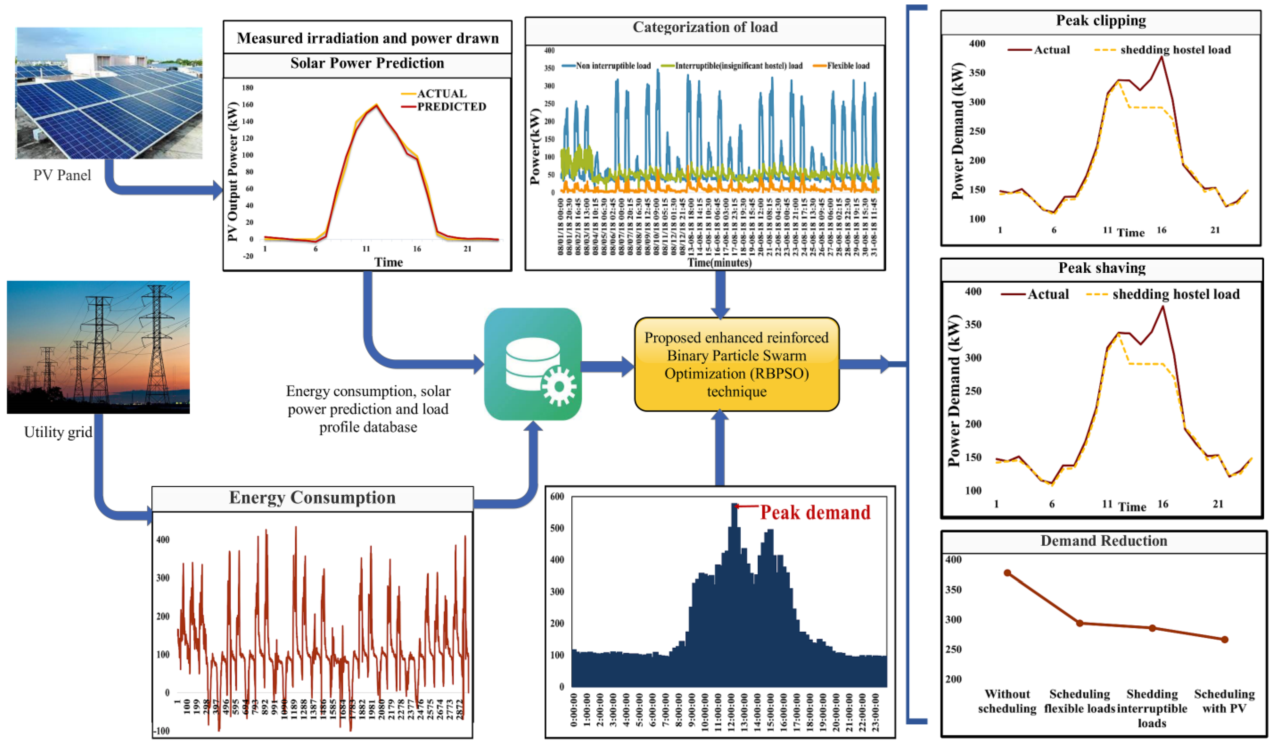
Proposed Scheme for Demand Management

As the smart grid has grown in popularity, DR has been developed to bridge the gap between supply and demand. The following is a summary of the most important contributions of this paper:

• MG-based residential power distribution is used in the demand management system;
• Considering the unpredictability of RERs, this study successfully uses the institution’s solar photovoltaic power capacity—calculated by the climate and historical data—to lower the need for utility power for an effective energy management system (EMS);
• To manage energy efficiently, machine learning (ML) model-based RFA-RM is developed using weather information with mathematical models for PV to forecast a generation profile of microgrids.
• The college’s real-time load data is gathered, and the load consumption during working hours and holidays is analyzed; the load data is divided into three groups depending on user preference and operation priority;
• The PSO algorithm is executed depending on the load pattern, using concepts such as time of usage, peak clipping, and valley filling techniques;
• The system evaluation is conducted by comparing the peak demand and PAR with conventional GA.

The paper has been structured as per the framework shown in Figure 1. One of the crucial factors of concern with respect to utility is peak demand management. On the other hand, consumers are concerned about energy cost reduction. The novelty of this study is attained via its proper scheduling of load to reduce the peak energy consumption by (1) load classification; (2) flexible shifting; and (3) peak clipping. The proposed method is performed by incorporating solar power to efficiently manage peak demand and balance load during peak hours.

Considering all three major load categories: interruptible, non-interruptible, and flexible load, as well as RES prediction for optimal DSM- the rest of the study, is organized as follows: Section 2 briefly describes challenges in power distribution and demand side management; Section 3 discusses the methodology and background of the study; Section 4 discusses the proposed distribution management strategy; and Section 5 discusses load categorization for demand management, concluding the study with results and discussion.

2. Challenges in Power Distribution and Demand-Side Management

Many developing nations continue to address supply and demand mismatches using conventional load-shedding strategies [23]. With recent advancements in industries, EV technologies have further increased electricity demand. Additionally, during peak times, the need for power is very high. Most residential and commercial loads still employ frequency-controlled automation, a traditional approach for load shedding that operates on a frequency rate or decrease. They may be simple to construct, but time delays slow their response and cause DG sources to trip. Programmable logic controllers (PLC)-based shedding is preferred over the under-frequency approach, which has certain drawbacks, including the lack of dual communication capability and predetermined or non-flexible power limits [24]. Controllable and non-controllable loads are considered in most research projects where consumer scheduling is carried out. The consideration of flexible load is minimal in the research area, and the institution-based load scheduling is even less than the residential load. Meeting peak demand is difficult for the utility, low-tension line (LT), high-tension line (HT), and other sectors. DR has established itself as an effective technique throughout the period by enabling the shedding and shifting of loads in response to grid demands while considering electricity imbalances and peak demand challenges [21]. Incorporating variable renewable energy sources such as solar and wind power into the power grid poses significant challenges. Renewables are not always available, and their power output can fluctuate rapidly due to weather conditions [14]. The study [25] proposes a scheme that utilizes probabilistic techniques to model the uncertainties associated with renewable energy sources, load forecasting errors, and other stochastic factors. To maintain stability in the face of disturbances, it is crucial to take the power system’s dynamic response into consideration. As a result, power distribution systems need to balance supply and demand effectively to ensure an uninterrupted power supply. Energy consumption and expenses are reduced by using more renewable energy sources. It is crucial to maintain adequate grid balancing to avoid problems such as overloading and blackouts as the integration of renewable energy sources continues to expand. This requires sophisticated forecasting and control systems that can anticipate changes in supply and demand and, based on this, adjust them accordingly.

2.1. Challenges in Peak Demand Management

Power-generating system scheduling is a vital topic in smart grids for successfully coordinating energy demand and generation. DR has been identified as a critical strategy for enhancing the efficiency of today’s power systems. Due to MGs’ low capacity, random power exchanges between the supplier and the loads may occur during regular operation, making maintaining operational capability and power quality challenging. Operating loads randomly and utilizing unexpected equipment may cause peak demand to be exceeded. Balancing the demand for electricity during peak periods against a limited supply requires careful planning and management. With many consumers demanding power at the same time, power distributors must work to reduce demand through demand response or other measures.

Expanding a power generation plant is costly and requires much investment and planning. In this regard, proper categorization of the load is necessary in order to execute DSM (i.e., peak clipping and valley filling). Peak demand poses significant challenges for power distribution and DSM, requiring careful planning, investment in infrastructure, and balancing supply and demand. Addressing peak demand is crucial for ensuring a reliable and sustainable power supply while minimizing environmental impacts. The prevailing intermittent characteristics of the RES have an impact on the planning and operation of electricity systems.

2.2. Consequences of Peak Demand and Need for Scheduling

The peak demand issue refers to the phenomenon when the demand for electricity reaches its maximum level during certain periods of the day, usually from morning to evening in the case of commercial loads. To maintain power balance at peak demand, the generation sector needs to increase the generation potential by expanding the plant capacity or installing new generation plants with increased demand. The need for power generation also increases. Numerous studies have examined the ideal day-ahead strategy for MGs, and a review of the literature shows that various quantitative and perceptual methods have been developed to address this issue [26]. The consideration of flexible load is minimal in the research area, and the institution-based load scheduling is even less than the residential load [27]. This sudden spike in demand can lead to strain on the power grid and supply system, which may cause power outages, brownouts, or even blackouts. Predicting peak demand can be challenging as it is affected by several factors, such as weather conditions, population growth, and consumer behavior, which are hard to anticipate. Despite the availability of energy storage solutions such as batteries, the amount of energy that can be stored during off-peak hours might not be sufficient to satisfy the demand during peak hours. In areas with inadequate infrastructure or an aging grid, it may be difficult to meet peak demand without overloading and damaging the network. Smart grid technologies are used to automatically balance energy supply as well as demand over peak hours. To address the peak demand issue, utility and energy companies must carefully manage the power grid and encourage energy conservation during peak hours [28]. Potential measures to address this challenge include the implementation of variable pricing strategies that motivate consumers to reduce electricity usage during peak periods, promoting the adoption of energy-efficient appliances that consume less power, and harnessing renewable energy sources that can provide clean and sustainable power during periods of high demand. In many countries, tariff rates fluctuate according to peak demand, resulting in higher power costs. Encouraging energy consumers to shift their usage to off-peak hours can prove to be challenging, as consumers may not be willing to change their behavior, especially if it disrupts their daily routines.

3. Methodology and Background of the Study

The energy infrastructure used in this research comprises RES (solar) with a primary grid and a backup generator. Figure 2 shows how current electricity is distributed in the microgrid. They may be simple to build, but deploying energy management and renewable energy sources can be costly, making it challenging to implement such solutions on a wide scale. Appliances can be classified into three categories—interruptible, non-interruptible, and flexible—based on their energy consumption, end-user preferences, and operational hours. Interruptible loads can be adjusted or turned off without impacting their performance. Flexible loads can change their operating hours to off-peak times, which helps reduce energy consumption and costs, considering the availability of solar power. MPP charge control is used to harness maximum power from the solar panels and store it in the battery.

Table 1. The main parameter of PV panel rating.

Parameter	Specification
Maximum power Rating (Wp)	310 W
Short circuit current (Isc)	8.90 A
Maximum power point current (Impp)	8.41 A
Maximum power point voltage (Vmpp)	37.0 V
Open circuit voltage (Voc)	44.9 V

shows the system parameters of solar panels made of TCE considered in this study [29].

3.1. Microgrid Pilot for Demand-Side Management

The smart grid is envisioned as a future energy infrastructure using several modern technologies [30]. An MG power distribution system comprises different dispersed energy resources. A microgrid is employed in [31], demonstrating that doing so not only boosts power consumption but also makes it possible to create a complementing and efficient network that may enhance dependability and voltage stability. It is now feasible to assure efficient power performance from generation sources to consumption, thus managing energy requirements. The ability to plan loads at the commercial level with the support of smart grid technology allows for cost- and energy-saving energy conservation and grid operating assistance in developing the best possible schedule out of the various options [28]. Thus, the smart grid provides consumers with a manual load scheduling system that is easy to set up and maintain, enabling them to evaluate the costs and advantages of various load plans. In an MG, the power consumption consists of the main load, controllable loads that can be switched off, and loads that can tolerate delays, such as flexible loads that can be postponed [32].

The study was conducted at Thiagarajar College of Engineering (TCE) in Tamil Nadu, Madurai district, at 9.8821° N and 78.0816° E. The area has a semi-arid tropical climate with hot, dry weather for eight months and average annual rainfall. From March through July, it becomes scalding. In February and March, there are cold winds. The city experiences pleasant weather from August to October, which includes frequent thunderstorms and heavy rain, and a somewhat wintry environment from November to February. The power distribution system on campus comprises various sources, including grid electricity, diesel generators, and solar photovoltaics. On the institution’s roof are installed SPV panels with a capacity of about 450 kW.

Thus, we have considered our institution for the execution of this proposed scheme as a pilot project. This can be employed in public, private, and residential/domestic premises to realize the DSM successfully. In contrast, the flexible loads in this work are scheduled with an available SPV system according to consumer satisfaction. Peak clipping tries to reduce supply during peak traffic. Utility companies accomplish this control by incentivizing consumers to avoid using power at peak times, actively managing rates, or imposing increased expenses. The approach is practical when there is no chance of establishing or upgrading existing power plants. This study demonstrates the necessity of SPV power for scheduling. The research site features a 450kW solar power system; however, only 30% of the PV electricity is used for consumption and utility. The peak demand can be decreased by using solar power and boosting consumption by just 10% of solar energy. Total load consumption in the institution during August (15-min dataset for accurate peak detection), where the overall peak demand reached around 570 kW on 10 August 2018 at 12:15:00 PM and the utility was unable to fulfill the total energy consumption. The details have been furnished in Figure 3 and Figure 4.

3.2. Realization of Peak Demand Management

Implementing a loaded schedule should be the first step in the electrical system design phase since it offers organization for reducing demand and conserving energy. Power monitoring and gathering all the data necessary to measure energy usage over time are essential to establishing a successful load-scheduling operation. Load shedding and load shaving are distinct strategies employed to regulate the supply and demand of electricity effectively. Load shedding intentionally interrupts the power supply to a certain area or group of customers during peak demand periods. This is usually conducted as a last resort to prevent the entire grid from collapsing. Conversely, load shaving entails decreasing or repositioning electricity usage during peak periods to circumvent the necessity for load shedding. This is achieved by using smart technology and flexible load scheduling. The user can identify massive burdens that are active at once. The EMS design is trained by utilizing past data, and the ideal solution was the load pattern of the daily curve [33]. A thorough knowledge of load variation is necessary to evaluate the effects of load management techniques, which are required for effectively and dependably scheduling energy usage. Based on the guidelines of the PSO algorithm, every identified member and particle continuously traverses a multi-dimensional search space that is regularly refreshed with the unique information possessed by each particle and its neighboring counterparts. The PSO method starts by analyzing a swarm of potential solutions. The particles that make up this swarm each offer an iterative solution, and this process continues until the objective function’s superior value is identified [32]. This optimization can resolve issues in an n-dimensional domain by utilizing points or surfaces as solutions. The peak demand reaches around 570 kW, but the utility demand is around 420 kW. Hence, the proper DSM is essential for the appropriate peak demand reduction. Controlled energy usage and comfort in a manner that modifies it by the actual pricing signal while considering human preferences [34]. Thus, in this scheduling, the SPV is implemented with accurate prediction, and to efficiently utilize this solar, the load is a category, and the peak shaving is conducted from peak hours to non-peak hours.

3.3. Role of Solar PV Systems in Peak Demand Management

The deployment of solar power is an excellent renewable waste alternative for power generation expansion resources. In DSM, random SP utilization will neither benefit peak demand reduction nor cost reduction. Therefore, the efficient prediction of solar power and its effective utilization during peak demand hours can lead to a reduction in energy consumption and peak demand. A DC–DC converter connects a solar-producing unit to a DC bus, allowing the system to function at full power. As they might leave a power system with inadequate capacity to satisfy load, the generator’s main benefit is its capability value to attain demand dependably. One of the critical benefits of PV systems in load scheduling is that they generate electricity during the day when energy demand is often highest [35]. The analysis determines a solar PV system’s electricity capacity [36] using the mathematical solution shown below in Equation (1).

$$S_{PV}\left(t\right)={\eta }^{PV}{a}^{PV}SI\left(t\right)[1-0.005\left(T\left(t\right)-25\right]$$

(1)

$${SP}_{PV}=\frac{1}{n}\left[\sum _{s=1}^n{Y}_s-Y_s^{^}\right]$$

(2)

Real-time information on SPV projections is collected using Equation (1) and energy management for appropriate microgrid concerns is assessed.This can lessen the probability of outages or other disturbances because power can be obtained locally rather than from centralized power facilities. S_PV stands for solar PV power, $\eta$ for efficiency of the panel, a for the area, and SI for Solar irradiation at time T. $Y_s$ stands for actual value, and $Y_s^{^}$ predicted value.

The maximum solar radiation is experienced from January through April, with a cumulative average value of 6.532015 (kWh/m²/day). The lowest value was observed for November at 3.10132647 kWh/m²/day. Irradiance is an essential component of PV performance, and inaccurate irradiance predictions directly impact the forecast’s accuracy and the availability of temperature. Figure 5 shows the variation in solar power production compared to wind speed and atmospheric temperature. Thus, the high temperature on the plane array results in a high PV output throughout the day. The prediction of natural solar energy with the above-mentioned equation is vital for the DSM. The availability of solar PV energy is necessary for variable load scheduling, which has advantages in terms of cost and utility sources. Figure 5 illustrates the solar irradiation and wind speed data of SPV utilized for the prediction process in the MLA, as described by Equation (2).

The current generated by the panel is almost constant. The voltage varies with respect to the irradiance and temperature, as shown in Figure 6. The voltage is operated at MPPT (maximum power point tracking). So, voltage is a continuously varying parameter. Hence, considering voltage and current separation for forecasting does not give appropriate results. Forecasting is conducted with power as a reference, with the power fluctuating with respect to weather conditions. Thus, the voltage is maintained as per the specification. The rated voltage of the solar panel considered in this work is 37.0 volts. The grid-tied inverter synchronizes the solar power with the grid for integration. The inverter switching control maintains the frequency profile. The frequency, as per the Indian standard, is 50 Hz [37]. Since voltage and frequency are not variable and have to be maintained as constants according to grid voltage and frequency, they have not been included in the constraint.

PV (photovoltaic) uncertainty can prevail due to various factors, including wind, shadows, cloudy conditions, etc. Thick cloud cover or cloudy conditions reduce the solar irradiance reaching the panels, resulting in lower energy production. The extent and duration of cloud cover can vary, making it difficult to predict solar power generation during cloudy periods accurately. Shadows cast on PV panels can significantly affect energy production. When shadows from nearby objects (such as buildings, trees, or other structures) fall on solar panels, they create variations in sunlight exposure across the panel surface. This causes partial shading, reducing the overall power output. The presence of shadows and clouds can introduce uncertainty in energy generation as it becomes challenging to predict the exact extent and duration of shading events. Accurate solar power prediction helps in estimating the available solar generation during peak demand periods. This PV uncertainty problem is solved by predicting solar power using the machine learning algorithm (MLA). In the RF algorithm-based selection technique, Figure 7 shows the solar power prediction with several inputs that result in an R-square value equal to 0.9. Figure 8 shows the solar power forecast at TCE with high prediction accuracy. By knowing the unexpected solar energy output, grid operators and utilities can better anticipate the level of available renewable generation and plan for the necessary balance between supply and demand as illustrated in Figure 9. The algorithm performs best compared to another neural network since the MLA algorithm is considered the most important feature to predict solar power under various meteorological conditions.

There is a connection between the primary grid and the AC bus. The AC and DC buses are interconnected via a bidirectional converter. Power converters work as inverters, converting power from DC to AC when the DC panel’s output exceeds the DC loads. It is analyzed that the peak consumption of the collected data goes beyond the limit, as shown in Figure 9; thus, flexible loads that are run during peak demand must be rescheduled to decrease their peak power usage.

4. Proposed Distribution Management Strategy

Load Model

Given the current tariff structure and load factors with predicted solar power data, the goal is to identify an ideal schedule to reduce the consumer’s power cost. A consumer’s premises are expected to run a variety of non-interruptible, flexible, and interruptible loads. Here, it is presumed that the utilities set the tariff so that users would change their load as the institution needed it, reducing the system’s maximum peak demand by implementing both solar power forecasting and the DSM algorithm, as illustrated by Figure 10. Demand policy solutions include implementing different tariff systems, such as time-of-use, high demand fees, and real-time tariffs. The tariff rate is peak consumption from 10 a.m. to 8 p.m., off-peak consumption from 11 p.m. to 7 a.m., and mid-peak consumption from 7 a.m. to 10 a.m. and 8 to 11 p.m. The individual load is represented as L = [cr1, …, cr5, nc1, nc2, fl1, fl2]. Because each day is partitioned into 24 equal time slots that begin at midnight with 24 h, where L represents the load operating during this period commencing at midnight for each hour represented by k (i.e., in slot k = 1 to slot k = 24), starting at midnight, with this time slot along with the available solar power, load scheduling is performed to minimize the peak demand. The problem relies on determining the best period in which for all loads to operate while meeting different limitations. The ON duration of the load is denoted as one by using BPSO to schedule the load to run on SPV power, as shown in

Table 2. Main variables for configuring optimization algorithms.

Parameter	GA	PSO
Population size	100	100
Generation/Iteration	100	100
Number of Variables	2	2
Weight	-	0.5
Mutation	0.8	-

.

The electrical supply in Figure 11 incorporates sustainable AC/DC sources and demands. To restrict the number of inverse conversions in a single AC or DC grid, this research recommended an AC/DC microgrid. Since a hybrid AC/DC grid’s energy management controls and operation are more complex than those of an individual AC/DC grid, researchers have looked at several operating modes for hybrid AC/DC grids. Coordination control strategies among numerous converters have been devised to maximize the energy generated from RES, limit the power transmission between AC and DC networks, and preserve the efficiency of both grids in the presence of fluctuating supply and demand. Consequently, one can successfully manage demand if the solar prediction is known before the high peak load scenario occurs. One could also save money by collecting electricity from the utility when needed and putting the rest of the time into a shutdown. PV energy resources aid customers’ participation in the electricity sector. Ref. [38] states that depending on the DR terms and conditions between the utility and the consumer, PV’s electricity can be used to power consumer electronics or sent back into the grid. Depending on the weather conditions, it is possible to schedule the load and receive information on solar DC power generation. Here, the study explores the available solar power and how to use it efficiently, minimizing the need for a utility under such circumstances. This study aims to analyze the available solar power, how to use it efficiently, and how to lessen the demand for energy in such cases. The essential item in prediction analysis is to help categorize learning data by detailing historical failures and performance and how much power may be saved by reducing convective loss. The load pattern model is adjusted after the generation prediction is completed. Our objectives and prerequisites areas follows:

• Classified loads and solar power generation are considered inputs;
• To categorize the load as interruptible, non-interruptible, and flexible;
• To find the peak demand duration and schedule the loads to the threshold limit;
• To integrate RER to satisfy load demand and meet peak demand;
• Load management and scheduling are conducted successfully using the predicted renewable energy data;
• To provide seamless power transfer across AC and DC lines under various generating and load scenarios.

5. Load Classification for Demand Management

Data classification categorizes information into numerous sorts, groups, or other unique categories. The total college demand is 700 kVA, a cumulative of two building blocks where one needs 400 kVA and the other has an order of 300 kVA. This study aims to lessen the 300 kVA demand peak, contributing to the institution’s overall peak demand. The division and dissemination of knowledge connected with dataset claims for different organizations or distinct aims are made possible by competence classification. Data concerning load in the research area (college) are gathered and examined. Non-interruptible loads, interruptible loads, and flexible loads are the types of loads collected. Figure 12 shows the graphical representation of the load categorization, where the three loads are operating without any DSM implemented.

(1)

Non-Interruptible Loads

A non-interruptible load refers to appliances or devices that cannot be easily adjusted, shifted, or turned off without affecting performance or causing disruptions. These loads require a continuous power supply and typically operate throughout the day without significant changes in their energy consumption patterns. Unlike interruptible or flexible loads, non-interruptible loads cannot be easily modified to reduce energy consumption or adjust operating hours. Even if the industry’s power supply has fallen, special measures are taken to preserve the stability of the power supply to these loads. The electrical lab, TCE main, ECE department, auditorium, and MCA are grouped as critical loads. The energy consumption of the non-interruptible load $C_{NIL}\left(k\right)$ is given by the following:

$$C_{NIL}\left(k\right)=\sum _{k=1}^{24}{S}_{NIL}\left(k\right)\times A_{NIL}\left(k\right)\times EP\left(k\right)$$

(3)

$$C_{NIL}\left(k\right)={\sum }_{k=1}^{24}{E}_{NIL}\left(k\right)\times EP\left(k\right),$$

(4)

where $S_{NIL}\left(k\right)$ denotes the ON/OFF condition for the time k, $A_{NIL}\left(k\right)$ denotes the entire consumed of non-interruptible load, and $E_{NIL}\left(k\right)$ denotes the overall power consumed of non-interruptible load.

(2)

Interruptible Load

“Interruptible load outlets” refer to redundant devices such as monitors and peripherals. They should be linked to non-essential load outlets so they may be turned off early to save battery life and allow for a steady shutdown of vital loads. Interruptible loads are loads of the ladies’ hostel and men’s hostel, which consider only the interruptible entertainment loads such as washing machines, pressing irons, vacuum cleaning, toasters, electric coffee, electric cookers, cloth dyers, and entertainment loads (i.e., stabilizers, television), excluding the essential loads such as lighting, fans, scanners, air conditioning, printers, photocopiers, and desktop computers. The consumption of the interruptible load $C_{IL}\left(k\right)$: (C_IL(k)):

$$C_{IL}\left(k\right)=\sum _{k=1}^{24}{S}_{IL}\left(k\right)\times A_{IL}\left(k\right)\times EP(k)$$

(5)

$$C_{IL}\left(k\right)=E_{IL}\left(k\right)\times EP\left(k\right),$$

(6)

where k is time, $A_{IL}\left(k\right)$ is the consumption of the equipment for time t, $EP\left(k\right)$ is the electricity power of the interruptible load for time slot t, $E_{IL}\left(k\right)$ is consideredto be the total consumption of interruptible load, and $S_{IL}\left(k\right)$ is the ON/OFF condition of the load status.

(3)

Flexible Loads

Flexible or intermittent loads often operate for less than 24 h. The precise time usually needs to be stated or acknowledged. The Pump House and STP Plant 2 are considered flexible loads.

$$C_{FL}\left(k\right)=\sum _{k=1}^9{S}_{FL}\left(k\right)\times A_{FL}(k)\times EP\left(k\right)$$

(7)

$$C_{FL}\left(k\right)=\sum _{k=1}^9{E}_{FL}\left(k\right)\times EP\left(k\right)$$

(8)

where $S_{FL}\left(k\right)$ denotes the ON/OFF status of the load for time slot of k (according to our study, the time slot considered for the flexible load to operate is 9 h based on lar power availability), $A_{FL}\left(k\right)$ is the consumption of flexible load appliances, and $E_{FL}\left(k\right)$ total consumption of the flexible load.

5.1. Objective Function

The proposed DSM schedules strive to optimize energy consumption by effectively shifting and adjusting loads to align the energy usage curve as closely as possible to an optimal state. The primary emphasis is on taking into account time slots and flexible loads as factors, trying to reduce the user’s power expenditure, particularly during times of peak demand when electricity rates are high. This approach seeks to enhance grid efficiency by optimizing energy consumption patterns.

$$Minimize:\sum _{k=1}^{24}\left(E_{NIL}\right(k)+E_{IL}\left(k\right)+E_{FL}\left(k\right)=\sum _{k=1}^{24}E\left(k\right)\times PR\left(k\right)$$

(9)

where PR denotes the price of electricity at time slot(k), and E is the total consumption.

5.2. Energy Balance Constraints

This ensures that the energy consumed by appliances, devices, or processes within the system is accounted for and balanced with the energy supply. Through the establishment of an energy balance, it becomes feasible to efficiently manage energy resources, prevent energy waste, and maintain stability and efficiency within the broader energy system. It is crucial to make sure that overall consumption does not surpass the sum of all electricity generated by solar panels combined with power imported from utilities.

$$\sum _{i=1}^n{P}_{PVi}^n+P_{UT}^n+P_{DG}^n=\sum _{i=1}^n{P}_{TL}^n$$

(10)

$$\sum _{i=1}^n{P}_G^n\ge P_{TL}^n+P_L$$

(11)

where $P_{PVi}$ stands for the solar power sources, $P_{UT}$ stands for the utility grid, $P_{DG}$ stands for the diesel generator, and $P_{TL}$ stands for total load.

5.3. Capacity Constrains

This constraint ensures that the utilization of resources remains within their predefined capacity limits to maintain system stability, efficiency, and sustainability. It helps prevent the overutilization or overloading of resources, which could lead to performance degradation, inefficiencies, or even failures. By considering the capacity constraint for resources, decision-makers and planners can appropriately allocate and manage resources to ensure their optimal utilization while avoiding any potential bottlenecks or constraints that may arise due to exceeding capacity limits.

$$P_{PVi,min}^n\le P_{PV}^n\le P_{PVi,max}^n$$

(12)

$$P_{UT,min}^n\le P_{UT}^n\le P_{UT,max}^n$$

(13)

$$P_{DG,min}^n\le P_{DG}^n\le P_{DG,min}^n$$

(14)

where $P_G^n$ is the total generation capacity at time n, and $P_L$ is the total line loss at time n. Equations (12)–(14) represents the generation capacity constraints of PV, Utility and, DG.

5.4. Operation Constraints

• It is observed that flexible loads operate during peak demand, and rescheduling the loads is crucial for lowering peak power usage;
• The load consumption shall not exceed the 300 KVA maximum load limit;
• A threshold of 270 kW is considered, at which all interruptible loads are clipped, and flexible loads are rescheduled to run at different times;
• The overall consumption is then computed, and an optimal solution is identified that minimizes the utility’s usage.

It is imperative to meet the power balance constraint in Equations (10) and (11) when scheduling different distributed power and non-dispatchable DER units. The surplus and deficit of electricity will be exported and imported to the utility to ensure that load and power generation are balanced at any given moment. It should exist within the minimum generation constraints to achieve the optimal schedule power levels. The DSM algorithm is constrained until convergence is conducted and its minimum value is attained, as shown in Figure 13. If the highest and lowest power constraints are exceeded, they are modified accordingly, as shown in Figure 14, where the flowchart and algorithm 1 explain the entire process of how the constraints and the DSM are implemented for this study.

5.5. Load Scheduling for Peak Power Reduction

Kennedy and Eberhart introduced PSO as a computer strategy for solving issues by repeatedly attempting to enhance a proposed solution in terms of a performance measure. Fish or birds’ schooling or flocking behavior served as the basis for the metaheuristic algorithm known as PSO [38]. The PSO method has a quicker convergence time, even though this issue comprises several facets and objective functions. However, it is incredibly flexible to circumstances with several objectives and purposes. Thus, the problem has several aspects and factors [39]. PSO stands out from other evolutionary systems in that it keeps every member of the population throughout the search phase and refrains from employing filtering processes such as crossover and mutation. The primary concept underlying PSO is that information is shared socially among people in a population—the PSO technique searches using an individual-corresponding population of particles, similar to evolutionary algorithms. In contrast to GA, no natural evolution operator is employed to provide novel solutions for the next generation. PSO, however, relies on individual knowledge exchange, which is why it is referred to as swarm intelligence. Every particle adjusts its place in the swarm through prior experience and the most superficial previous position. The particle accumulates knowledge by keeping track of its ideal personal circumstance, exhibiting both a local and a global search depending on nearby expertise or the prowess of the swarm. Global neighbor and local neighbor iterations were used in constructing the PSO algorithm. The algorithm 1is provided below for a clear process of load scheduling.

The gbest model represents the best particle in the whole swarm, and each particle’s best prior location migrates toward the global neighborhood model. In the local variant known as the Pbest model, each particle seeks the best place from its previous visit and the finest particle in its small neighborhood. PSO has been successfully used in several applications, including task management, variable spring systems, and power and voltage regulation. It is possible to represent problem-solving using swarms of particles. In the beginning, the particles are scattered randomly over the solution space. The particles are first dispersed arbitrarily throughout the global area. The ideal location and the position of the best-performing particle affect how they move across the solution space.

The repeatedly evaluated performance of the particles is assessed using a fitness function. If the particle arrives at its ideal location, indicated by Pbest, and the position of the lightest particle, designated by gbest, the velocity and position are updated using the following equation at each iteration step. The following equation then updates the position and velocity at all iteration phases.

$$V_i^{(k+1)}={wV}_i^k+{c1}^{\ast }rand()({pbeat}_i^k-x_i^k)+{c2}^{\ast }rand()({gbest}_i^k-x_i^k)$$

(15)

$$x_i^{(k+1)}=x_i^k+V_I^{(K+1)}$$

(16)

where c1 and c2 denote the acceleration coefficient (i.e., they maintain a balance between individual and neighboring behavior).

5.6. Binary Particle Swarm Optimization

For separate particles, the fundamental PSO algorithm employs continuous values. Particle specifications in discrete space are required to organize the loading procedure. The velocity update equation is used in the discrete version of BPSO, and the velocity is limited to a range. Then, each particle’s present location and velocity are updated. Evaluation is once again conducted to determine the fitness of the particles in the swarm. A sigmoid function with the following definition is then used to transfer the velocity to [0, 1].

$$S\left(V_i^{\left(k+1\right)}\right)=\frac{1}{1+{(e}^{{-V}_i^{(k+1)}})}$$

(17)

$$x_i^{(k+1)}=\left\{\begin{array}{l}1,ifS\left(V_i^{\left(k+1\right)}\right)>rand()\\ 0,Otherwise\end{array}\right.$$

(18)

5.7. Load Scheduling Algorithm

Step 1: Initialization of the algorithm parameters such as the decision variable (DV), weight coefficient, and population size (Pop), and data on solar prediction, maximum demand limit, and load details;

Step 2: Loading of the data and electricity traffic rate for the considered categories;

Step 3: The new particle is generated by updating the velocity;

Step4: The position of the particle is updated by Equation (15);

Step 5: The best particle position (pbest) and the global best position (gbest) are updated;

Step 6: The ith particle’s fitness is determined;

Step 7: If fitness(i) is less than pbest(i) and the peak load limit is not exceeded for the present position, pbest is equal to fitness and saves the particle’s location;

Step 8: The global best particle position is saved if pbest(i) is smaller than gbest and gbest = pbest(i);

Step 9: We establish a maximum and lowest range for the velocity values, and then use a sigmoid function to map the velocity with s(vi);

Step 10: We set the new particle location only inside the allowed subset;

Step 11: We continue from step 3 until the allotted iterations have been achieved (Algorithm 1).

Algorithm 1: Proposed particle swarm optimization (PSO)

1: Initialization of algorithm parameters 2: Initialization of population size 3: Pop = 1:tp 4: Initialization of load data 5: L = $\left[\begin{array}{ccccc}{NIL}_{K=1}& \dots \dots & {IL}_{K=1}& \dots \dots & {FL}_{k=1}\\ :& & :& & :\\ :& & :& & :\\ :& & :& & :\\ :& & :& & :\\ :& & :& & :\\ {NIL}_{k=24}& \dots \dots & {IL}_{k=1}& \dots \dots & {FL}_{k=1}\end{array}\right]$ 6: Uc (: ,: ,pop)=[cr1 cr2 cr3 cr4 cr5 nc1 nc2 f1 f2]; 7: Objective function is calculated 8: Peakconsumption (pop) = sum(eb(tp,:,pop)) + sum(eb(tp,:,pop)) 9: Offpeakconsumption(pop) = sum(eb(tp,:,pop)) + sum(eb(tp,:,pop)); 10: Midpeakconsumption(pop) = sum(eb(tp,:,pop)); 11: sol(pop,49) = (peakconsumption(pop)*PR*H) + ((offpeakcon sumtion(pop))*PR*H) + (midpeakconsumption(pop)*PR*H); 12: Check the threshold limit 13: if eb(i,:,pop) >= 280 14: count = count + 1; 15: sol(pop,50) = count; 16: Update the velocity and position 17: $V_i^{(k+1)}={wV}_i^k+{c1}^{\ast }rand()({pbest}_i^k-x_i^k)+{c2}^{\ast }rand()({gbest}_i^k-x_i^k)$ 18: $x_i^{(k+1)}=x_i^k+V_I^{(K+1)}$ 19: Update best position particle 20: if 21: fitness ($x_i^{(k+1)}$) < $fitness\left({pbest}_i^k\right)$ then, 22: ${pbest}_i^k$ = $x_i^{(k+1)}$ 23: End 24: Update global best position 25: if 26: $fitness\left({pbest}_i^k\right)$ < ${gbest}_i^k$ then, 27: ${gbest}_i^k$ = ${pbest}_i^k$ 28: Checking the stopping criteria, for iteration count, go to step 9, 29: End

6. Result and Discussion

6.1. Role of Solar Power Prediction and Utilization

The high-accuracy prediction of solar power using the MLA (regression) is considered for the scheduling of loads calculated from Equation (2). The average irradiation normally increases at about 11 a.m. before declining, and energy consumption during these hours witnesses an increasing trend [17]. Solar irradiance and ambient temperature affect how much power a PV system can create. These two factors can change at any moment. The irradiation-based solar power drawn from TCE is depicted in Figure 15 [26]. The upcoming average hourly prediction series is based on past data collection. Figure 8 displays the modeling findings of solar power prediction. For the increasing power demand to avoid the harshest effects of peak electricity cost minimization, the solar power generation forecast is a crucial requirement. This prediction of solar power in the past would result in the reduced utilization of utility power and cutting bills by using the renewable energy source to its benefit. Effective utilization of solar PV power optimizes usage during time off traffic to reduce energy costs. Based on the proposed method, the peak demand is achieved to reduce the utility’s power, thereby minimizing peak power costs.

6.2. Effect of DSM on Consumption

Utilizing load shifting allows customers to change their consumption habits to off-peak times based on affordable rates. It consists of both peak clipping and peak shaving [39]. Critical equipment can only be stopped or turned off after operating. Users’ comfort will be adversely affected if they are delayed or moved after the procedure has begun since they function at set power ratings. The inputs comprise load statistics from institutions categorized based on priority and solar power generation with load prioritization techniques. Flexible loads are only used occasionally; non-critical loads should have an intermittent power source, and critical loads should have a continuous power source. The loads have been assigned according to their priority.

A load curve or load profile graph depicts the change in demand or energy load over time. Figure 16 illustrates the power consumption without DSM implementation. As described in Figure 12 and

Table 3. DSM scheduling based on the appliance categories for commercial load consideration.

Category of Appliance	Name of Appliance	Scheduling Criteria
Non-interruptible load (non-shiftableload)	All college load (electrical lab, TCE main block, ECE department, Auditorium, and MCA).	Operating for all hours without any interruption
Interruptible load (considering only shiftable load)	Lady’s and Men’s hostel (entertainment loads washing machines, pressing iron, vacuum cleaning, toasters, electric coffee, cooker, cloth dyers, entertainment loads i.e., stabilizers, television, etc.,).	Initially on for all hours. On the peak demand condition, the peak clipping is performed.
Flexible load	Pump house and STP Plant2 (pumps in water supply, wastewater treatment)	Randomly operating based on solar power availability.

, the model’s measurements include information on temperature and solar energy prediction, and the threshold limit and base load profiles are used to determine the pattern of dispatchable loads.

6.3. Effect of Load Shifting

Depending on the estimated horizon, equipment that can change its power capabilities without compromising user comfort can be modified. Building demand flexibility and managing a building’s adaptable resources shift the load pattern to accommodate different needs without compromising end users’ interests [40]. The load rescheduling was intended to use solar power and reduce peak demand when the solar irradiation is greater. The simulation’s findings indicate that the flexible load shifts within a day’s 24 h.

Figure 17 illustrates how load shifting makes it possible to schedule devices from peak hours 2 to 4 to non-peak hours between 9 and 1 h while achieving fewer energy savings. Flexible load scheduling is carried out to reduce peak demand by shifting the loads during the low-demand period by 22%. The flexible load scheduling was carried out with GA, which resulted in 19%. The flexible load scheduling resulted from the conditions in Figure 17a,b, where the peak demand was also reduced from 294.05 kW in the case of PSO to 303.23 kW in GA.

6.4. Effect of Peak Clipping

It has been stated that utilities deploy load shedding to stop the flow of electricity when supply cannot keep up with the sharp spike in demand [41]. Despite having rated power, the gadgets, including washing machines and dishwashers, are adaptable and may be shut down, moved, or rescheduled as needed. The power consumption is reduced by the DSM technique using peak clipping; thus, in Figure 18a,b, the performance of both algorithms is similar, but PSO provides the best result. In the GA algorithm, the iteration time is too long compared to the PSO. The peak clipping process shows that the load profile has significantly improved, as shown in Figure 18a of PSO with 24%, i.e., from 378.06 KW to 285.75 KW. Peak clipping was conducted utilizing BPSO and a significant quantity of energy from an SPV source, and the results demonstrate greater applicability. The particle swarm optimization approach is used under these presumptions, and an optimal solution is obtained by activating flexible loads and altering the particle’s velocity. The overall consumption is then computed, and an ideal solution that decreases utility use is determined. Excess loads are switched off at peak hours in the clipping scheme to reduce energy consumption. The microgrid oversees the delivery of non-interruptible loads, which are regarded as non-shiftable loads.

Power production companies use this information to predict how much energy they will need at any given moment. Figure 16 illustrates a load curve, such as a load duration curve. The usage of capacity over time is shown by the load curve. This graph indicates the lower consumption during peak hours by rescheduling the flexible loads to non-peak hours with PV (i.e., if the loads are run randomly during peak periods, it might lead to higher usage), as seen in Figure 16. Scheduling is performed while adhering to the specified threshold limit, as depicted in Figure 18c. The comparison between the graphs with and without scheduling demonstrates that the flexible load is shifted, and the interruptible hostel load is reduced during periods of peak demand. Additionally, peak shifting is implemented to ensure that the peak remains within the prescribed limit. In a conventional scheme, the peak has violated the specified limit. This violation causes very big challenges for the utilities. So, employing flexible and interruptible loads, MATLAB v. 2022a simulations of load shifting and shedding, taking solar production into account, were run. The main grid’s peak demand was reduced by around 29%. The results show that the total power demand has decreased from 378.06 kW to 266.546 kW with solar power generation. The maximum and minimum values of power consumed within 24 h per threshold limits are displayed in

Table 4. Summary of the statistical value of comparing and evaluating PSO and GA.

Statistical Value	Actual Value	GA			PSO
		Load Shifting	Peak Clipping	Scheduling with PV	Load Shifting	Peak Clipping	Scheduling with PV
Maximum power (kW)	378.06	303.23	299.02	270.54	294.05	285.75	266.54
Minimum power(kW)	108	108	108	108	108	108	108
Peak-to-peak power(kW)	270	195.23	191.02	162.54	186.05	177.75	158.54
Mean power(kW)	326.45	302.745	290.64	281.51	302.745	378.96	156.42
Median (kW)	326.45	312.79	268.42	165.9	302.74	263.79	134.7
PAR	1.8602	1.002	1.0288	0.9608	0.9056	0.754	0.7211

. Table 4 summarizes the evaluation parameters before and after the DSM approach with PSO and GA. A larger PAR denotes a bigger disparity between the peak and average demand, suggesting a greater possibility for a decrease. By implementing strategies that successfully lower the peak demand while maintaining an acceptable level of average demand, the PAR can be reduced.

There are more loads in commercial MGs, and they have a longer consumption period; it involves the use of smart technology to monitor electricity usage, identify periods of peak demand, and automatically shift energy consumption to times when demand is low. Both utilities and customers may benefit from a more dependable and economical energy system by employing DSM on a loaded schedule. To effectively implement DSM, the loads are shifted from peak to non-peak hours. The loads in this study are categorized according to consumption and usage time, respectively. As a result, the influence of DSM and renewable energy sources such as SPV on the creation of MG and the acquisition of power from the primary grid may be significantly reduced. Thus, using various population sizes and several iterations, the model is run repeatedly, which results in scheduling within the threshold limit, as shown in

Table 5. Demonstration of percentage decrease during the demand peak.

Load Curve	GA	Peak Demand Reduction in Percentage for GA	PSO	Peak Demand Reduction in Percentage for PSO
Without scheduling	378.06	-	378.06	-
Scheduling flexible loads	303.23	19%	294.05	22%
Shedding interruptible loads	299.02	20%	285.75	24%
Scheduling with PV	270.54	27%	266.54	29%

.

Ensuring the stability and dependability of the grid is DSM’s main goal. By minimizing the PAR, one method is used to accomplish this. Figure 19 shows a histogram that contrasts the PAR of demand profiles created before and after the implementation of DSM using two distinct methods. The PAR values for the demand profiles are presented visually in the histogram and Table 5 to allow for a clear comparison between the two situations: PSO and GA. The variations in PAR between the two procedures are easily understood thanks to this graphical depiction from Figure 19. Prior to the implementation of DSM, the original demand profile had a PAR of 1.8602. However, after applying the clipping and shifting techniques in the DSM process, the PAR values decrease significantly to 0.905 and 0.754, respectively. The peak reduction from Table 5 results indicates that the GA also performs well compared to PSO and the difference is also less, but PSO is able to attain the threshold limits.

7. Conclusions

This research has mainly focused on modeling the use of DSM techniques and optimizing the operation of microgrids by defining optimization issues. An enhanced reinforced binary particle swarm optimization (RBPSO)of the grid-connected PV system of an institutional building by employing renewable energy resources has been proposed, implementing peak clipping and valley filling methods. Considering the high penetration of PV systems, this paper estimates renewable energy prediction using RFA-RM. Due to the difficulty of having all the power sources available simultaneously, hybrid microgrid systems require a continuous power supply to the grid. This integration can also enable demand-side management programs that encourage consumer participation and engagement, leading to more sustainable and efficient energy consumption patterns. Flattening the load profile, reducing the impact of intermittent generation, and boosting system effectiveness are all possible benefits of a successful demand-side management strategy. Flexible load scheduling reduces the stress on the electrical grid during periods of high demand, thereby reducing the risk of blackouts and other issues. By moving consumption to the time of day when energy is cheapest, it also helps to lower the cost of power. Our experiments and implementation show the necessity and importance of including PV prediction in DSM scheduling. On the other hand, with this DSM approach, energy consumption is optimized, with a peak demand reduction from 378.06 kW to 266.54 kW. The following conclusions are summarized:

• Utilizing on-site generation such as solar panels and implementing the BPSO to satisfy the consumer with priority-based load scheduling during peak periods is minimized;
• The DSM method has a lower peak demand compared to a system without DSM;
• The peak demand reduction of 22% is obtained during flexible load shaving with DSM based on a tariff;
• The shedding of interruptible loads results in a significant peak demand reduction of 24%;
• The scheduling of loads during peak demand, coupled with the utilization of solar photovoltaic (PV) power, has led to a significant reduction of 29% in peak demand.

Load shifting in the DSM process resulted in a smaller reduction in the PAR compared to other techniques. This can be observed from Figure 19, where the generated peak power consumption after the DSM shows a relatively smaller decrease in PAR in the case of PSO (0.721), which is better than 0.960 in the case of GA. The computational results show that the suggested machine learning prediction approach combined with enhanced BPSO provides an efficient solution for institutions regarding load scheduling, energy conservation, and decreasing system expenses. The utility infrastructure is used to satisfy the energy demand in this situation (intermittent weather), and the recommended scheme’s anticipated SPV power delivery strategy is used to reduce costs. When solar power production exceeds demand, the utility compensates for the surplus energy. Hence, based on the availability of solar power, the load is scheduled for where the utility cost at the time is not required, which results in a cost reduction. Integrating solar prediction and PSO algorithms for load scheduling presents a promising approach to enhancing the efficiency and effectiveness of load-scheduling processes. Therefore, the government, utilities, and individuals need to consider DSM as a viable strategy for managing energy consumption and promoting sustainable energy practices. Reduced microgrid power usage ensures grid stability and, as a result, reduces costs.

References

1. Zieba Falama, R.; Ngangoum Welaji, F.; Dadjé, A.; Dumbrava, V.; Djongyang, N.; Salah, C.b.; Doka, S.Y. A solution to the problem of electrical load shedding using hybrid pv/battery/grid-connected system: The case of households’ energy supply of the northern part of Cameroon. Energies 2021, 14, 2836. [Google Scholar] [CrossRef]
2. Dashtdar, M.; Flah, A.; Hosseinimoghadam, S.M.S.; Kotb, H.; Jasińska, E.; Gono, R.; Leonowicz, Z.; Jasiński, M. Optimal Operation of Microgrids with Demand-Side Management Based on a Combination of Genetic Algorithm and Artificial Bee Colony. Sustainability 2022, 14, 6759. [Google Scholar] [CrossRef]
3. Kakran, S.; Chanana, S. Smart operations of smart grids integrated with distributed generation: A review. Renew. Sustain. Energy Rev. 2018, 81, 524–535. [Google Scholar] [CrossRef]
4. AlDavood, M.S.; Mehbodniya, A.; Webber, J.L.; Ensaf, M.; Azimian, M. Robust Optimization-Based Optimal Operation of Islanded Microgrid Considering Demand Response. Sustainability 2022, 14, 14194. [Google Scholar] [CrossRef]
5. Habibifar, R.; Khoshjahan, M.; Saravi, V.S.; Kalantar, M. Robust Energy Management of Residential Energy Hubs Integrated with Power-to-X Technology. In Proceedings of the 2021 IEEE Texas Power and Energy Conference, TPEC, Online, 2–5 February 2021. [Google Scholar] [CrossRef]
6. Ali, S.; Khan, I.; Jan, S.; Hafeez, G. An optimization based power usage scheduling strategy using photovoltaic-battery system for demand-side management in smart grid. Energies 2021, 14, 2201. [Google Scholar] [CrossRef]
7. Hein, K.; Xu, Y.; Gary, W.; Gupta, A.K. Robustly Coordinated Operational Scheduling of a Grid-Connected Seaport Microgrid under Uncertainties. IET Gener. Transm. Distrib. 2021, 15, 347–358. [Google Scholar] [CrossRef]
8. Roslan, M.F.; Hannan, M.A.; Jern Ker, P.; Begum, R.A.; Indra Mahlia, T.M.; Dong, Z.Y. Scheduling Controller for Microgrids Energy Management System Using Optimization Algorithm in Achieving Cost Saving and Emission Reduction. Appl. Energy 2021, 292, 116883. [Google Scholar] [CrossRef]
9. Li, H.; Wang, Z.; Hong, T.; Piette, M.A. Energy flexibility of residential buildings: A systematic review of characterization and quantification methods and applications. Adv. Appl. Energy 2021, 3, 100054. [Google Scholar] [CrossRef]
10. Dranka, G.G.; Ferreira, P. Load flexibility potential across residential, commercial and industrial sectors in Brazil. Energy 2020, 201, 117483. [Google Scholar] [CrossRef]
11. Ahmad, A.; Khan, A.; Javaid, N.; Hussain, H.M.; Abdul, W.; Almogren, A.; Alamri, A.; Niaz, I.A. An optimized home energy management system with integrated renewable energy and storage resources. Energies 2017, 10, 549. [Google Scholar] [CrossRef] [Green Version]
12. Tulabing, R.; Yin, R.; DeForest, N.; Li, Y.; Wang, K.; Yong, T.; Stadler, M. Modeling study on flexible load’s demand response potentials for providing ancillary services at the substation level. Electr. Power Syst. Res. 2016, 140, 240–252. [Google Scholar] [CrossRef] [Green Version]
13. Sarker, E.; Halder, P.; Seyedmahmoudian, M.; Jamei, E.; Horan, B.; Mekhilef, S.; Stojcevski, A. Progress on the demand side management in smart grid and optimization approaches. Int. J. Energy Res. 2021, 45, 36–64. [Google Scholar] [CrossRef]
14. Philipo, G.H.; Kakande, J.N.; Krauter, S. Neural Network-Based Demand-Side Management in a Stand-Alone Solar PV-Battery Microgrid Using Load-Shifting and Peak-Clipping. Energies 2022, 15, 5215. [Google Scholar] [CrossRef]
15. Kerboua, A.; Boukli-Hacene, F.; Mourad, K.A. Particle swarm optimization for micro-grid power management and load scheduling. Int. J. Energy Econ. Policy 2020, 10, 71–80. [Google Scholar] [CrossRef]
16. Malekshah, S.; Malekshah, Y.; Malekshah, A. A Novel Two-Stage Optimization Method for the Reliability Based Security Constraints Unit Commitment in Presence of Wind Units. Clean. Eng. Technol. 2021, 4, 100237. [Google Scholar] [CrossRef]
17. Prabpal, P.; Kongjeen, Y.; Bhumkittipich, K. Optimal battery energy storage system based on VAR control strategies using particle swarm optimization for power distribution system. Symmetry 2021, 13, 1692. [Google Scholar] [CrossRef]
18. Menos-aikateriniadis, C.; Lamprinos, I.; Georgilakis, P.S. Particle Swarm Optimization in Residential Demand-Side Management: A Review on Scheduling and Control Algorithms for Demand Response Provision. Energies 2022, 15, 2211. [Google Scholar] [CrossRef]
19. Kennedy, J.; Eberhart, R. Particle Swarm Optimization. In Proceedings of the ICNN’95-International Conference on Neural Networks, Perth, WA, Australia, 27 November–1 December 1995. [Google Scholar]
20. Rezaee Jordehi, A.; Jasni, J. Particle swarm optimisation for discrete optimisation problems: A review. Artif. Intell. Rev. 2015, 43, 243–258. [Google Scholar] [CrossRef]
21. Abd Elsadek, E.M.; Ashour, H.A.; Hamdy, R.A.; Sedky, M.M.M. An Approach of Load Management and Cost Saving for Industrial Production Line Using Particle Swarm Optimization. Mansoura Eng. J. 2020, 45, E37–E44. [Google Scholar] [CrossRef]
22. Latif, U.; Javaid, N.; Zarin, S.S.; Naz, M.; Jamal, A.; Mateen, A. Cost Optimization in Home Energy Management System Using Genetic Algorithm, Bat Algorithm and Hybrid Bat Genetic Algorithm. Proc. Int. Conf. Adv. Inf. Netw. Appl. AINA 2018, 2018, 667–677. [Google Scholar] [CrossRef]
23. Sepehrzad, R.; Moridi, A.R.; Hassanzadeh, M.E.; Seifi, A.R. Intelligent Energy Management and Multi-Objective Power Distribution Control in Hybrid Micro-grids based on the Advanced Fuzzy-PSO Method. ISA Trans. 2021, 112, 199–213. [Google Scholar] [CrossRef] [PubMed]
24. Philipo, G.H.; Chande Jande, Y.A.; Kivevele, T. Clustering and Fuzzy Logic-Based Demand-Side Management for Solar Microgrid Operation: Case Study of Ngurudoto Microgrid, Arusha, Tanzania. Adv. Fuzzy Syst. 2021, 2021, 6614129. [Google Scholar] [CrossRef]
25. Malekshah, S.; Alhelou, H.H.; Siano, P. An Optimal Probabilistic Spinning Reserve Quantification Scheme Considering Frequency Dynamic Response in Smart Power Environment. Int. Trans. Electr. Energy Syst. 2021, 31, e13052. [Google Scholar] [CrossRef]
26. Alawode, B.O.; Salman, U.T.; Khalid, M. A flexible operation and sizing of battery energy storage system based on butterfly optimization algorithm. Electronics 2022, 11, 109. [Google Scholar] [CrossRef]
27. Yeo, J.; Wang, Y.; An, A.K.; Zhang, L. Estimation of Energy Efficiency for Educational Buildings in Hong Kong. J. Clean. Prod. 2019, 235, 453–460. [Google Scholar] [CrossRef]
28. Wang, C.; Zhang, Z.; Abedinia, O.; Farkoush, S.G. Modeling and analysis of a microgrid considering the uncertainty in renewable energy resources, energy storage systems and demand management in electrical retail market. J. Energy Storage 2021, 33, 102111. [Google Scholar] [CrossRef]
29. Muniyandi, V.; Manimaran, S.; Balasubramanian, A.K. Improving the Power Output of a Partially Shaded Photovoltaic Array Through a Hybrid Magic Square Configuration with Differential Evolution-Based Adaptive P&O MPPT Method. J. Sol. Energy Eng. Trans. ASME 2023, 145, 1–14. [Google Scholar] [CrossRef]
30. Souhe, F.G.Y.; Mbey, C.F.; Boum, A.T.; Ele, P. Forecasting of Electrical Energy Consumption of Households in a Smart Grid. Int. J. Energy Econ. Policy 2021, 11, 221–233. [Google Scholar] [CrossRef]
31. Bouakkaz, A.; Andrés, J.; García, M.; Haddad, S.; Andrés Martín-García, J.; Gil-Mena, A.J.; Jiménez-Castañeda, R. Optimal Scheduling of Household Appliances in Off-Grid Hybrid Energy System using PSO Algorithm for Energy Saving. Int. J. Renew. Energy Res. 2019, 9, 427–436. [Google Scholar]
32. Hemmati, M.; Mohammadi-Ivatloo, B.; Abapour, M.; Anvari-Moghaddam, A. Day-ahead profit-based reconfigurable microgrid scheduling considering uncertain renewable generation and load demand in the presence of energy storage. J. Energy Storage 2020, 28, 101161. [Google Scholar] [CrossRef]
33. Li, B.; Shen, J.; Wang, X.; Jiang, C. From controllable loads to generalized demand-side resources: A review on developments of demand-side resources. Renew. Sustain. Energy Rev. 2016, 53, 936–944. [Google Scholar] [CrossRef]
34. Okwu, M.O.; Tartibu, L.K. Particle Swarm Optimisation. Stud. Comput. Intell. 2021, 927, 5–13. [Google Scholar] [CrossRef]
35. Varudharajulu, A.K.; Ma, Y. A Survey on Big Data Process Models for E-Business, E-Management, E-Learning, and E-Education. Int. J. Innov. Res. Comput. Commun. Eng. 2018, 738–744. [Google Scholar] [CrossRef]
36. Mohammadpour Shotorbani, A.; Zeinal-Kheiri, S.; Chhipi-Shrestha, G.; Mohammadi-Ivatloo, B.; Sadiq, R.; Hewage, K. Enhanced real-time scheduling algorithm for energy management in a renewable-integrated microgrid. Appl. Energy 2021, 304, 117658. [Google Scholar] [CrossRef]
37. Frequency Control in a Power System. Available online: https://eepower.com/technical-articles/frequency-control-in-a-power-system (accessed on 31 July 2023).
38. Sørensen, L.; Lindberg, K.B.; Sartori, I.; Andresen, I. Analysis of residential EV energy flexibility potential based on real-world charging reports and smart meter data. Energy Build. 2021, 241, 110923. [Google Scholar] [CrossRef]
39. Javaid, N.; Hussain, S.M.; Ullah, I.; Noor, M.A.; Abdul, W.; Almogren, A.; Alamri, A. Demand side management in nearly zero energy buildings using heuristic optimizations. Energies 2017, 10, 1131. [Google Scholar] [CrossRef] [Green Version]
40. Leonori, S.; Martino, A.; Frattale Mascioli, F.M.; Rizzi, A. Microgrid Energy Management Systems Design by Computational Intelligence Techniques. Appl. Energy 2020, 277, 115524. [Google Scholar] [CrossRef]
41. Amer, A.; Shaban, K.; Gaouda, A.; Massoud, A. Home Energy Management System Embedded with a Multi-Objective Demand Response Optimization Model to Benefit Customers and Operators. Energies 2021, 14, 257. [Google Scholar] [CrossRef]
Figure 1. The framework of the proposed method.
Sustainability 15 12209 g001
Figure 2. The layout of the current microgrid architecture.
Sustainability 15 12209 g002
Figure 3. Total peak demand consumption.
Sustainability 15 12209 g003
Figure 4. The total load consumption vs. the utility.
Sustainability 15 12209 g004
Figure 5. Monthly solar irradiation, atmosphere temperature, and wind speed variation at TCE.
Sustainability 15 12209 g005
Figure 6. The framework of forecasting (input and output values).
Sustainability 15 12209 g006
Figure 7. Summary of the OLS regression-trained model for solar power prediction using MLA.
Sustainability 15 12209 g007
Figure 8. Shows TCE’s forecasted power consumption on an hourly average (kW).
Sustainability 15 12209 g008
Figure 9. Total demand for solar power generation vs utility grid.
Sustainability 15 12209 g009
Figure 10. The brief flowchart proposed considering MLA with PSO.
Sustainability 15 12209 g010
Figure 11. Block diagram for the proposed DSM with RES in a hybrid microgrid.
Sustainability 15 12209 g011
Figure 12. The load curve classification (non-interruptible and interruptible loads and flexible loads).
Sustainability 15 12209 g012
Figure 13. The best solution for the convergence curve.
Sustainability 15 12209 g013
Figure 14. Particle swarm optimization flowchart.
Sustainability 15 12209 g014
Figure 15. Comparison between the irradiance (W/m2) and temperature with solar power drawn at TCE.
Sustainability 15 12209 g015
Figure 16. The actual power consumption before applying the DSM technique.
Sustainability 15 12209 g016
Figure 17. Load curve for scheduling (a) Flexible load1 (Pump house); (b) Flexible load2 (Sewage Plant).
Sustainability 15 12209 g017
Figure 18. Load profile of actual data with scheduling of flexible load and peak clipping with (a) PSO algorithm, (b) GA algorithm, and (c) the scheduling without and with DSM.
Sustainability 15 12209 g018aSustainability 15 12209 g018b
Figure 19. PAR value of load shifting, clipping before and after DSM for two approaches: (a) PAR value for GA; (b) PAR value for PSO.
Sustainability 15 12209 g019