Urban Waste Management and Prediction through Socio-Economic Values and Visualizing the Spatiotemporal Relationship on an Advanced GIS-Based Dashboard

Abstract

Enhancing data-driven decision-making is vital for waste authorities. Although few studies have explored the influence of socio-economic indicators on waste tonnage, comprehensive analysis of urban waste data focusing on geographical information is also scarce. There is a dearth of dashboards for visualizing waste tonnage with spatial relationship maps. This study aims to present a prediction model useful for estimating urban waste by using personal income (I), the number of income earners (E), land values (L), the estimated resident population (P) and population density (D), called the IELPD measures. An innovative approach is developed to identify the correlation between urban household waste data and socio-economic factors and develop an advanced dashboard based on a geographic information system (GIS). To accomplish this, relationship maps and regression analysis are deployed to visualize household waste data spanning six years of waste production in New South Wales, Australia, classified into three categories: recyclable, residual and organic (RRO) wastes. Furthermore, this classification enables accessing the association between these three waste categories and the IELPD metrics. And there are four types of visualization generated, that is, thematic mapping, spatial relationship maps, correlation matrices and dashboard development. The regression analysis shows a substantial association between RRO waste tonnage, population changes and a minor correlation with land values. Overall, this study contributes to urban waste data storytelling and its spatiotemporal associations with socio-economic determinants. This paper offers a valuable prediction model of the IELPD metrics to estimate urban waste and visualize them in a dashboard allowing practitioners and decision-makers to track trends in the RRO waste stream in urban waste generally.

1. Introduction

Urban waste is known as a significant source for recycling and reuse as key pillars of circular economy. To achieve these objectives, an urban solid waste collection system was [1] developed with recycling performance evaluation and analysis, which considered various geometrics around retail services. Moreover, research [2] of rural solid waste systems assessed environmental impacts using lifecycle assessment, especially investigating landfill gas between waste collection, treatment, and utilization. An assessment of waste impact at macro levels revealed that large waste quantities pose a potential threat to the environment by causing pollution or disease transmission. In 2018, the World Bank estimated that global waste generation would increase from 2.01 billion UK tons in 2016 to 3.4 billion tons by 2050. Moreover, the estimate indicated that the cost of environmental and health damage from poor waste management in low- and middle-income regions was around USD375 billion per year [3]. Poor waste management is likely to trigger underground water pollution and soil contamination from landfill sites. According to the World Health Organization [4], unsafe water, poor sanitation, and inadequate hygiene cause an estimated 2 million deaths per year.

The efficient management of urban waste may minimize the environmental footprints of inhabitants. Among various wastes, household waste management has the potential for a high level of circularity since it facilitates reuse, recycling, and recovery over disposal. Waste management is vital for eco-friendly development and increased circularity [5]. In addition, the circular economy contributes significantly to environmental preservation objectives [6]. To enhance urban waste management, it is essential to investigate the existing context of the various categories of municipal and regional household waste. Urban planners and decision-makers need to monitor the amount of waste generated over time and utilize the sophisticated tools available to visualize the many categories of household waste in space, such as recyclables and organics. This information will be essential for data-driven, well-informed urban waste management decision-making.

According to Australia’s national waste stream profile [7], waste is classified into three categories based on its source. Commercial and industrial waste (C&I), construction and demolition waste (C&D), and municipal solid waste (MSW) are the three categories. MSW consists of waste collection by councils (local government) from households. When the waste stream is divided to single out the MSW, it should first pass through the two major categories of waste before accessing household waste, which are C&D waste and C&I waste. Household waste in urban areas was classified into three basic groups: recyclable, residual (biodegradable and nonbiodegradable), and organic (biodegradable), together called the RRO waste.

In the context of urban metabolism, MetaExplorer—a digital platform developed in Portugal [8]—serves a crucial role in facilitating the sustainable energy transition by providing comprehensive energy data. Additionally, the platform encompasses thematic areas pertinent to waste management within national socio-economic metabolism. With potential digital technologies, The University of Sydney, et al. [9] studied the case of NSW, including data visualization and analytics of precincts and infrastructure in terms of space and time, enabling scenario assessment with a focus on circular economy metrics.

Once circular material flows in the industry are implemented, minimizing waste, utilizing resources more efficiently, reusing, and recycling products also contribute significantly to the lowering of carbon emissions from urban waste. As more and more information became visible of the actual waste stream, the rate of waste recycling for environmental protection was constantly mentioned.

By providing more transparency of the waste stream, data-driven decision-making can support a deeper understanding of the current and historical situation, helping to make better judgments and placing a more efficient emphasis on waste recycling for environmental protection. Moreover, the significance of data-driven decision-making originates from the fact that data-derived information supports deeper understanding of the current situation and, as a result, better decision-making.

Accessibility to essential data, such as waste statistics, is likewise a core issue and demand in this context. In addition to data preparation, the analysis of such datasets is essential for exploring patterns, trends, and insights. Digital tools such as dashboards provide decision-makers with the opportunity to view these insights at-a-glance in terms of space and time. Household waste data collection is a demanding and time-consuming task, since such data are dispersed across organizations that do not provide public access to them, as so many entities are involved in collecting household waste at various levels of governance. Even if the information is collected, processing such data is time-consuming and requires extensive pre-processing since the datasets are stored in various file formats. In waste management, data analytics involves examining unstructured data to uncover previously unknown linkages and other insights through trend analysis. Organizations and waste management companies can utilize analytics to explain, anticipate, and enhance their operations, as Niska, et al. [10] mentioned.

Some official documents from the federal government in Australia, such as the National Waste Report [11,12,13] and National Waste Policy Action Plan [14,15], emphasize the importance of digitalization in waste data management in Australia. The word clouds of these reports are visualized based on the word frequency in Figure 1. This initiative will provide an interactive waste data management platform for government and industry. The policy may require the presentation of a proof-of-concept platform or the visualization of waste flow. The ‘Waste Data Hub’ is being improved by the Federal Waste Authority, and Microsoft Power BI was used to construct the ‘National Waste Data Viewer’ dashboard [16], which is categorized by source stream, material category, time, jurisdiction, and waste facilities.

The current dashboards’ prediction functionality and trend analysis capabilities are limited. Current access to waste data allows users to view the spatial relationship between social and economic indicators. The tonnage of urban household waste, associated with the population and households, could be used directly for social studies to track personal income and income earner numbers for their socio-economic characteristics. As one study mentioned [17], the municipal solid waste management transition focused on Chinese cities with different population sizes and considered multiple metrics, including finance, land, administrative control, tax revenue and subsidies. Such studies embraced population size, land, and tax revenue in solid waste studies. The connection between waste tonnage and metrics is one of the reasons why the study chose four parameters related to waste generation: land, population, income, and the number of income earners [18]. Furthermore, community characteristics such as land values, land use in urban and regional areas, and waste management are based on land values rather than personal income in the local community. The spatial relationship between socio-economic metrics and the tonnage of waste generated, play an important role in assessing the impact of locational information and neighbourhood analytics. Based on the year-to-year changes in socio-economic metrics, the tonnage of waste can be assessed with temporal change from the spatial level.

While the dynamic representation of past data in dashboard diagrams is very useful, the inclusion of spatial analysis insights from the data is rare. This study fills this gap by using spatial relationship maps to build a dynamic and innovative smart waste visualization dashboard (SWVD) for NSW. This paper analyses household waste data from 2014 to 2019 and specifies spatiotemporal associations between the RRO waste and IELPD metrics, using correlation matrices and relationship map methods.

2. Review of Urban Waste Relationships, Digital Platforms, and Policies

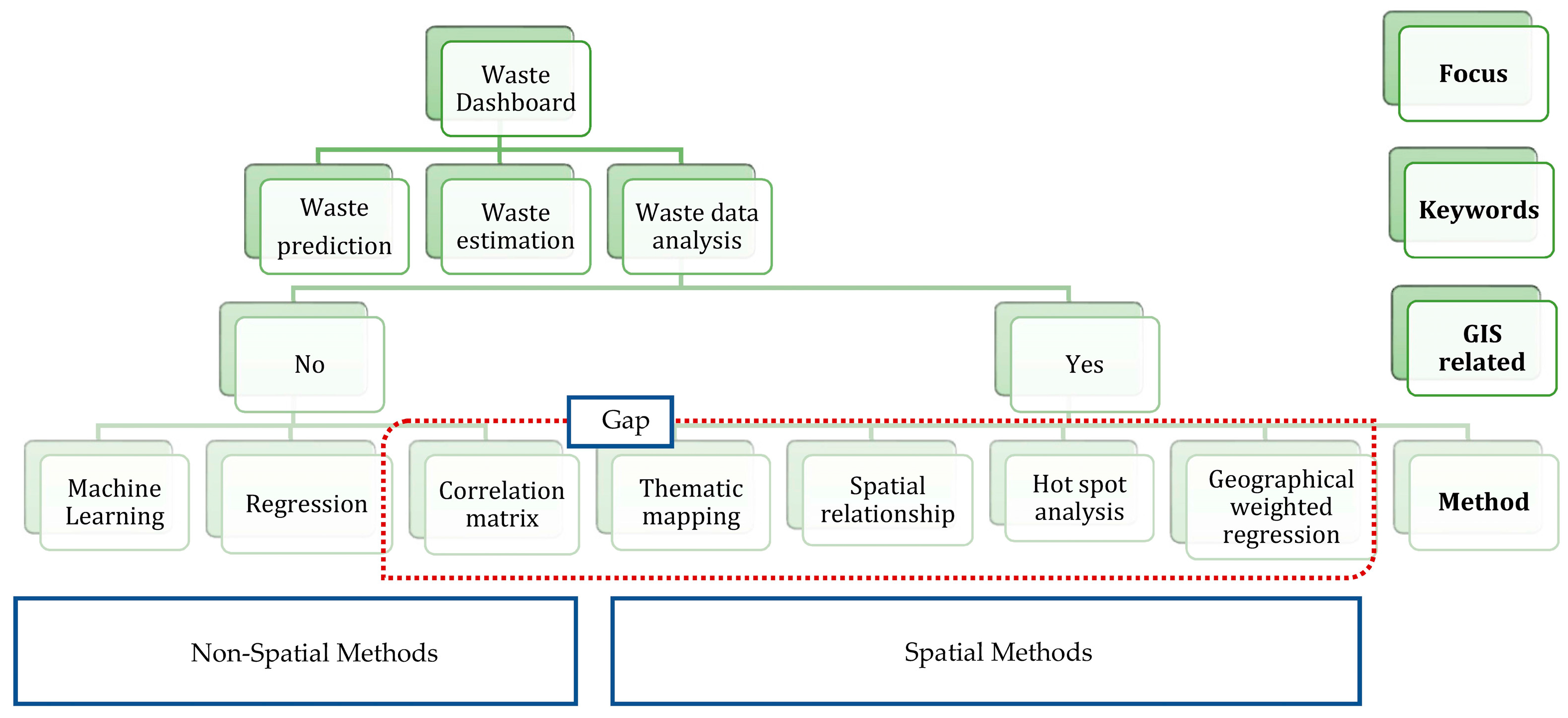
GIS-based data are typical location-based data that visualize spatial distribution patterns. Figure 2 present a summary of research methods for waste management and spatial analysis. GIS is known as a useful tool for analysing waste’s spatiotemporal relationships and visualizing waste changes over time. Some researchers have investigated the spatial relationship of waste collection stations and their temporal impacts on neighbours. For instance, Yang, et al. [19] proposed the spatial and temporal analysis of illegal dumping in municipal solid waste evaluations, considering social indicators such as income, unemployment, and population density.

Exploring the temporal relationship between waste tonnage and related variables depends on regression analysis methods, particularly multiple linear regression, and Pearson regression techniques. For instance, researchers developed heuristic route planning algorithms for waste pickup vehicles in Greater Melbourne [20]. The study utilized Python libraries and ArcGIS mapping to simulate neighbourhoods and designed a chart-based intelligent bin system in Wyndham City Council.

For exploring spatial relationships, Smith, et al. [21] research employed approaches from social epidemiology datasets to study the spatial relationship between the outbreak of COVID-19 and construction in Sydney and Melbourne. To consider the patterning of disease among entire populations and other metrics, including environment, economy, and government policies, the relationship map and clustering analysis must be employed in order to connect these metrics together to explore spatial patterns before and after COVID-19.

Figure 2 shows the correlation matrix and machine learning, which is generally considered in the research of multiple influencing factors. For instance, the researcher of [22] collected historical bushfires and meteorological and vegetation datasets to explore the relationships and interactions over the past 40 years. To achieve the relationship exploration in space and time, He, et al. [22] applied multiple linear regression and Bayesian logistics to model the probability of forest fire occurrence. The correlation matrix shows the importance of each influencing factor in multiple linear regression.

Focusing on waste research, metropolitan waste collection areas were divided into suburbs, Local government areas (LGAs) or municipal governments. Local government areas collect household waste from each bin on a building, at the community level. Rare datasets for waste tonnage optimization and regional recycling rate improvements are linked. Thus, waste estimation through potential impact factors in regions is a popular data science topic for waste management. For instance, a study [23] uses machine learning to estimate municipal waste. This method forecasts weekly and daily waste generation at the property level for 609 subsections of new work city from the department of sanitation over ten years. Weather, building type, density, and demographic variables are included. Data limitations may reduce machine learning’s prediction accuracy, however, requiring incremental improvements.

Some studies highlighted the significance of using appropriate modelling techniques for the predictive analysis of environmental impact in agricultural systems. Ghasemi-Mobtaker, et al. [24] proposed that wheat farm production should be developed using mathematical and artificial intelligence modelling, which could predict the economic profit, global warming potential (GWP) and output energy. It provides insights into the relationship between inputs and outputs in agricultural production.

In this agricultural study [25], the researchers considered diesel fuel, biocides, input costs and the cost of different operations in 75 wheat farms with modelling techniques including life cycle assessment (LCA), artificial neural networks (ANNs), and adaptive neuro-fuzzy inference system (ANFIS) methods. Nabavi-Pelesaraei, et al. [25] suggested using these methods, especially ANNs and ANFIS, to solve the optimization of energy consumption and estimate the yield of agriculture products without plant farming.

In a large agricultural system, environmental impacts [26] need to be evaluated for toxicity factors and exergy analysis to identify the demands of water systems. Multiple factors analysis generally needs analytic hierarchy processes to identify metrics’ priority in complex systems.

There are temporal, topographical, and observational correlations between RRO waste. Apartment occupants gather recyclables from nearby areas [27,28]. The property owner develops and controls these collecting facilities mandated by the Australian cadastral parcel. Local councils collect green, red, and yellow bins by ‘colours’, and ‘materials’ [29]. It is characterized by yellow for recycling, green bins for organic waste, and red bins for rubbish, categorized in this study as residual.

For waste research across social and economic parameters, researchers [30] suggested that the variation of waste disposal factors is associated with the mass of biomedical waste in Regina, Canada. The study used Python Seaborn data visualizations such as Boxplots, Violin Plots, and Joint plots to analyse the tonnage of waste. As a result, the amount of monthly waste disposal was 450–550 tons/month. Compared to the pre-COVID-19 era, monthly waste data were less available, and seasonal influences on total waste disposal were less clear before the COVID-19 pandemic.

In Australia, the waste collection management system displayed the waste tonnage of city council datasets and the vehicle’s route. RRO waste is listed in the mesh block of several local government areas in the open-source workbook available from the NSW EPA. Smart waste management was analysed with the challenges for a sustainable circular economy in an Indian study [31]. The research utilized a comparative analysis between the qualitative phase of government employees and quantitative analysis to identify the barriers to the implementation of smart waste management.

After waste data collection, the researcher assesses neighbourhood spatial linkages between spatial visualization and regression analysis in household waste. Using weighted regression, morphological and residential dispersion is analysed. A Campania study compared mountain town waste collection with the impact of land characteristics [32], especially how morphology and housing distribution affect separate waste collection (SWC) in mountain communities. In sparsely populated regions, socio-economic variables support the large geographical variation of land characteristics. Similarly, Richter et al. [33] reveal that numerous sources have previously optimized the cost-effectiveness of waste management. These studies employ geospatial or temporal analysis to investigate the neighbourhood environmental impacts. Based on these studies, it can be reflected that rare studies identified the statistical correlation and spatial relationship among year-to-year waste tonnage and socio-economic metrics in same geographical areas. There are multiple indicators that influence the amount of waste generation such as personal income, number of income earners, land values, population, and population density. In the study mentioned above [17], disposal management transition was defined as the process of transition from traditional methods of municipal solid waste (MSW), including landfill and incineration. Municipal solid waste in Chinese cities can identify the effects of disposal management transition and its determinants, including population size, per capita GDP, per capita road area, and number of tourists. These metrics were developed to predict the carbon reduction in MSW disposal. One study [1] of urban solid waste management in aggregating performance indicators mentioned the number of retail services in the assessment models.

The dashboards of vehicles indicate speed, oil, and water temperature in real-time. A ‘dashboard’ in business provides fast views of KPIs related to a goal or business process. The dashboard is a visual representation of a ‘process report’ in maps and infographics so that internet dashboards for the COVID-19 pandemic since 2020, display active cases, immunization rates, and regional patterns. Dashboards for regional government, covering architecture, engineering, construction, urban planning, and emergency services, are expanding. Dashboards have been developed at several infrastructure levels in city management. The dashboard displays real-time data so that drivers may immediately respond to incidents [34]. It has tools for monitoring and assisting decision-makers, such as statistical graphs and geographic maps [35].

In these dashboards, developers generally visualize real-time statistics on maps and diagrams, including Sydney’s dashboard [36]. These features also exist in one of the most popular COVID-19 cases, a real-time dashboard from John Hopkins University [37]. Meanwhile, the researcher [37] found more issues. Several options for expanding the prototype’s functions emerged. The researchers emphasize interactive reporting to access historical or real-time geocoded data through 1D diagrams, 2D maps and 3D scenes. Meanwhile, socio-economic metrics are to be displayed in the local communities. Examples of waste management dashboards from the literature evaluation and industry investigations are shown in

Table 1. Summary of the state-of-the-art practices in developing the waste dashboards.

Name	Dash or Map with ‘Tools’	1D/2D/3D 1 + Real-Time/Historical	Limitations and Deficiencies	With Social Metrics
Victoria’s waste projection model [38]	Dash, Microsoft Power BI	2D + Historical	Without spatiotemporal analysis	Yes
Victoria’s local government waste data dashboard [39]	Dash, Microsoft Power BI	2D + Historical	Without spatiotemporal analysis	No
Domestic waste and recycling dashboard in WA [40]	Dash, Microsoft Power BI	1D + Historical	Without spatial analysis	No
Smart city waste management with SAP Analytics Cloud [41]	Dash, SAP Analytics and ESRI	2D + Real-time	Without spatiotemporal analysis	No
Map of waste and recycling centres [42]	Map, Google Map	2D + Historical	Without temporal analysis	No
Waste streams (Roboat) [43]	Dash, Mapbox+ OSM	2D + 3D + Realtime	Without spatiotemporal analysis	No
National waste reporting mapping tool [44]	Map, Geoscience Australia tool	2D + Historical	Without temporal analysis, more qualitative	No
Waste and resource recovery data hub—national waste data viewer [16]	Dash, Microsoft Power BI	2D + Historical	Without spatiotemporal analysis	No
August 2022 waste metrics dashboard [45]	Dash, report PDF	2D + Historical	With spatiotemporal analysis, but display without interactivities	No
NSW Jobs and Businesses In waste management and recycling [46]	Dash, Flourish Studio	2D + Historical	Without temporal analysis	Yes
Zero waste data dashboard [47]	Dash, Microsoft Power BI	1D + Historical	Without spatial analysis	No
Solid waste tonnage dashboard [48]	Dash, Microsoft Power BI	1D + Historical	Without spatial analysis	No

¹ 1D: Diagram (diagram view), 2D: Map + diagram (map view), 3D interactive diagram map (scene view). Note: ‘Realtime’ refers to current or ongoing tracking, and ‘historical’ refers to data covering a few years saved in digital storage. Source: compiled by the authors, 2023.

.

Due to the popularity of the ‘smart city’ concept, waste management is undergoing a digital transformation, such as with city council or EPA waste stream data. The national waste report is illustrated graphically. However, these waste management datasets were not chosen for digital display and real-time analysis in the interactive mapping app. This current work will identify the temporal changes in waste tonnage and social, economic metrics from 2014 to 2019, and perform spatial visualization and relationships in RRO waste with multiple social metrics, develop an SWVD of annual household waste in NSW from 2014 to 2019.

3. Materials and Methods

3.1. Study Area and Data

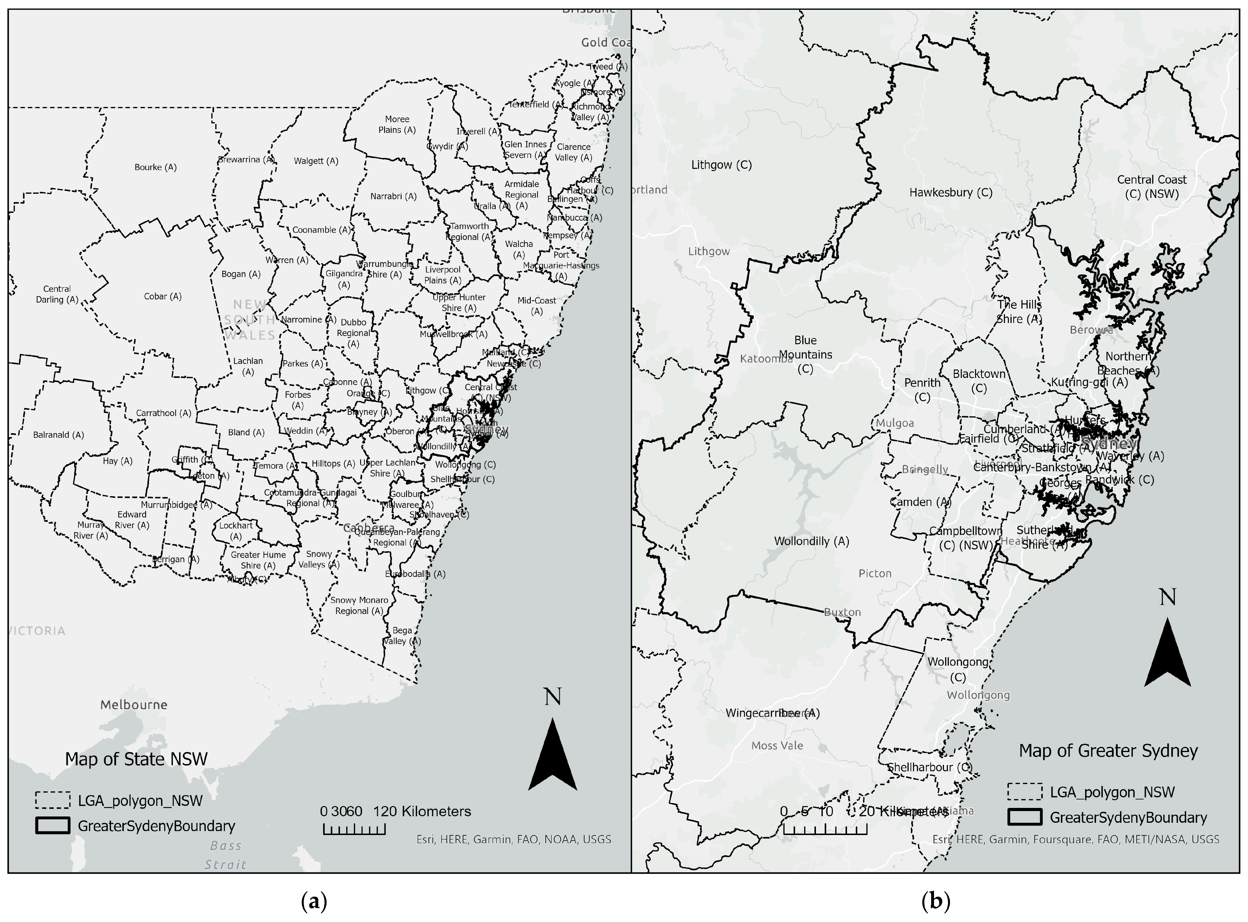
This study aims to develop a GIS-based technique for monitoring and analysing waste as part of its overall mission. New South Wales (NSW) was selected as a case study for the implementation of the visualization method, including Greater Sydney, as shown in Figure 3. The map is based on the coordinate system of GDA2020 MGA Zone 55. The figure displays the geographical range from NSW in Figure 3a to Greater Sydney in Figure 3b. The area in NSW that is not included in the Greater Sydney area is called the ‘Regional NSW’.

NSW has a larger population and superior garbage databases compared with other Australian jurisdictions. However, no research has been undertaken on relationship maps to help with educated household waste decisions. NSW is located on Australia’s East Coast. In 2020, NSW was the most populous state in Australia, with 128 LGAs. There are three types of RRO waste streams, and the data profile, format, and sources are displayed in

Table 2. Data profile, including the waste datasets from NSW.

Name	Format	Data Source	Location Information in the Dataset	Temporal Information in a Period
Local council waste and resource recovery data 1*	XLSX	Environmental Protection Authority of NSW	Polygon-LGA	2014–2019
Land values	XLSX	NSW Spatial Services	Point-Suburb	1996–2021
Estimated resident population (ERP)	CSV/XLSX	Australian Bureau of Statistics (ABS)	Polygon-LGA	2001–2021
The personal income and number of earners	CSV/XLSX	ABS Income (Including government allowances), LGAs, 2014–2019	Polygon-LGA	2014–2019
ERP density 2*	CSV/XLSX	ABS	Polygon-LGA	2001–2021

Sources: compiled by the authors, 2023. Note: ¹* This study for waste tonnage datasets in EPA from 2014 to 2019 is shown in the original files for 2014–2015, 2015–2016, 2016–2017, 2017–2018, 2018–2019, and 2019–2020. One year gap value uses 2019–2020 minus 2018–2019 data, which means waste tonnage changes from year to year. The five-year gap is followed by similar waste tonnage changes from 2014 to 2019. ²* Estimated Resident Population Density uses Estimated Resident Population divided by the LGA in km².

.

3.2. Methods

This study aims to conduct a spatiotemporal analysis of the NSW waste data with socio-economic metrics between 2014 and 2019.

Table 3. Methodology summary through the research objectives (Source: compiled by the authors).

Research Objectives	Data	Methods and Tools
Analyse the variance of waste-related social metrics and RRO waste between 2014 and 2020 by location at the LGA level.	Residual, organic, recyclable	Thematic mapping (Jenks natural break)
Identify the spatial relationship between the level of IEPLD, and the amount of produced waste in the three types of RRO waste.	Residual, organic, recyclable	Relationship map (Quantile breaks), Pearson correlation, Spearman correlation
Develop a dashboard with visualization, cross-interactive maps, and insights from waste stream data.	Personal income, number of income earners, land values, ERP, ERP density, residual, organic, and recyclable.	ArcGIS experience builder

shows the specific methods and data used for achieving each objective in this research.

As seen in Table 3, methods of spatial visualization in different social economics, a relationship map, and a correlation matrix are implemented in this research to achieve the objectives. These methods are explained below after describing data preparation.

3.2.1. Data Preparation and Processing

Geocoding helps to visualize spatial data. For GIS specialists, Feature Manipulation Engine (FME) software (version 2021.1.0.1) can convert file formats and geocode datasets. The geocoder for FME can locate the nearest address using ArcGIS Online, Google, ArcGIS Online and ArcGIS Pro were used to join geographical features of maps geocoded from several LGAs. There are insufficient monthly and daily public datasets for high-resolution spatial analysis. Although the EPA’s annual data collection on MSW and C&D waste is limited by commercially sensitive datasets, the RRO waste data can be reviewed annually in the household waste from ‘Local council waste and resource recovery data’. Green bins, yellow bins, and red bins have been recognized categories for RRO waste since 2005. Reclassification of time series datasets indicates RRO inefficiency. Since the smallest unit of information was, the city council in the datasets obtained, the update of the LGA geographical boundary impacted spatial visualization and the examination of relationships within LGAs. Spatial visualization is less explicable when a classification contains missing data (null values). In addition, the processing of spatial data enables the connection of household waste patterns within municipal solid waste jurisdictions.

In the meantime, the model builder in ArcGIS Pro optimizes the pre-processing of data joins across different datasets. Identifying regional correlations between RRO waste and other socio-economic variables can reduce software operating time and permit data processing. Pearson regression enhanced the regression of numerous socio-economic components. Using data cleaning, the yearly data frame is transformed into several columns, including various annual datasets, such as the attribute table of the residual recycle layer in GIS, particularly residual waste recycling from 2014 to 2019.

For thematic mapping in multiple metrics, there are two methods mentioned in this study, such as Jenks natural breaks and quantile breaks. Jenks natural breaks classify ranked numerical data by considering multiple nonuniform classes with varying frequencies of observations per class. On the other hand, quantile breaks use a different distribution method to evenly classify the observed values into multiple class intervals, resulting in uneven class distances but an equal frequency of observed values per class.

3.2.2. Relationship Map

Bivariate choropleth maps [49], known as relationship maps, were customized to reveal spatial patterns of areas’ cross-overlap and divergence in several waste types. Using ArcGIS online or ArcGIS Pro, an analyst can compare two columns of datasets by selecting one column and then selecting the ‘relationship’ mapping style from the symbology section of layers. This method is to determine whether there is a spatial relationship between a RRO waste tonnage and IELPD in this research.

3.2.3. Regression Analysis

(1)

Pearson correlation

Pearson correlation is beneficial for displaying the correlation heatmap among multiple indicators in the research. It expresses the importance of correlation among multiple parameters at the neighbourhood level [50,51].

Equation (1) The metric of Pearson Correlation

$$\mathsf{\rho }=\frac{{\sum }_{\mathrm{i}=1}^{\mathrm{n}}({\mathrm{x}}_{\mathrm{i}}-\overline{\mathrm{x}})({\mathrm{y}}_{\mathrm{i}}-\overline{\mathrm{y}})}{{[{\sum }_{\mathrm{i}=1}^{\mathrm{n}}{({\mathrm{x}}_{\mathrm{i}}-\overline{\mathrm{x}})}^2{({\mathrm{y}}_{\mathrm{i}}-\overline{\mathrm{y}})}^2]}^{0.5}}$$

(1)

where:

$\overline{\mathrm{x}}$, $\overline{\mathrm{y}}$ are the mean of x, y, which are representatives of urban household waste data and one of the four urban data factors (i.e., land value, number of income earners, personal income, and ERP, ERP density).

The range of Pearson’s regression, which assesses the correlation between two numeric features, is from −1 to 1. It is the ratio between two variables’ covariance and standard deviation products. The value ‘+1’ denotes the highest positive correlation, while ‘0’ denotes the absence of a linear relationship, and ‘−1’ denotes a perfect negative linear relationship.

For a better visual representation of the outcomes of Pearson’s correlation, a correlation heatmap [22] is generated. Positive cell values denote a positive relationship, while negative cell values denote a negative relationship. Correlation heatmaps can be used to identify potential relationships between variables and assess the strength of these correlations.

(2)

Spearman regression

The Spearman’ rank correlation is to study the nonlinear relationship between two variables. It is defined similarly to the Pearson correlation for variables, which is nonnormalized distribution in spatial scales [52]. The categories of correlation [53] were evaluated to rank correlation coefficients as follows: (a) The coefficient is greater than 0.7, called a well-correlated metric; (b) the coefficient is between 0.5 and 0.7, called a moderate correlated metric; (c) the coefficient is between 0.3 and 0.5, called a weak correlated metric; (d) the coefficient is less than 0.3, called a slight correlated metric.

3.2.4. Development of a GIS-Based SWVD

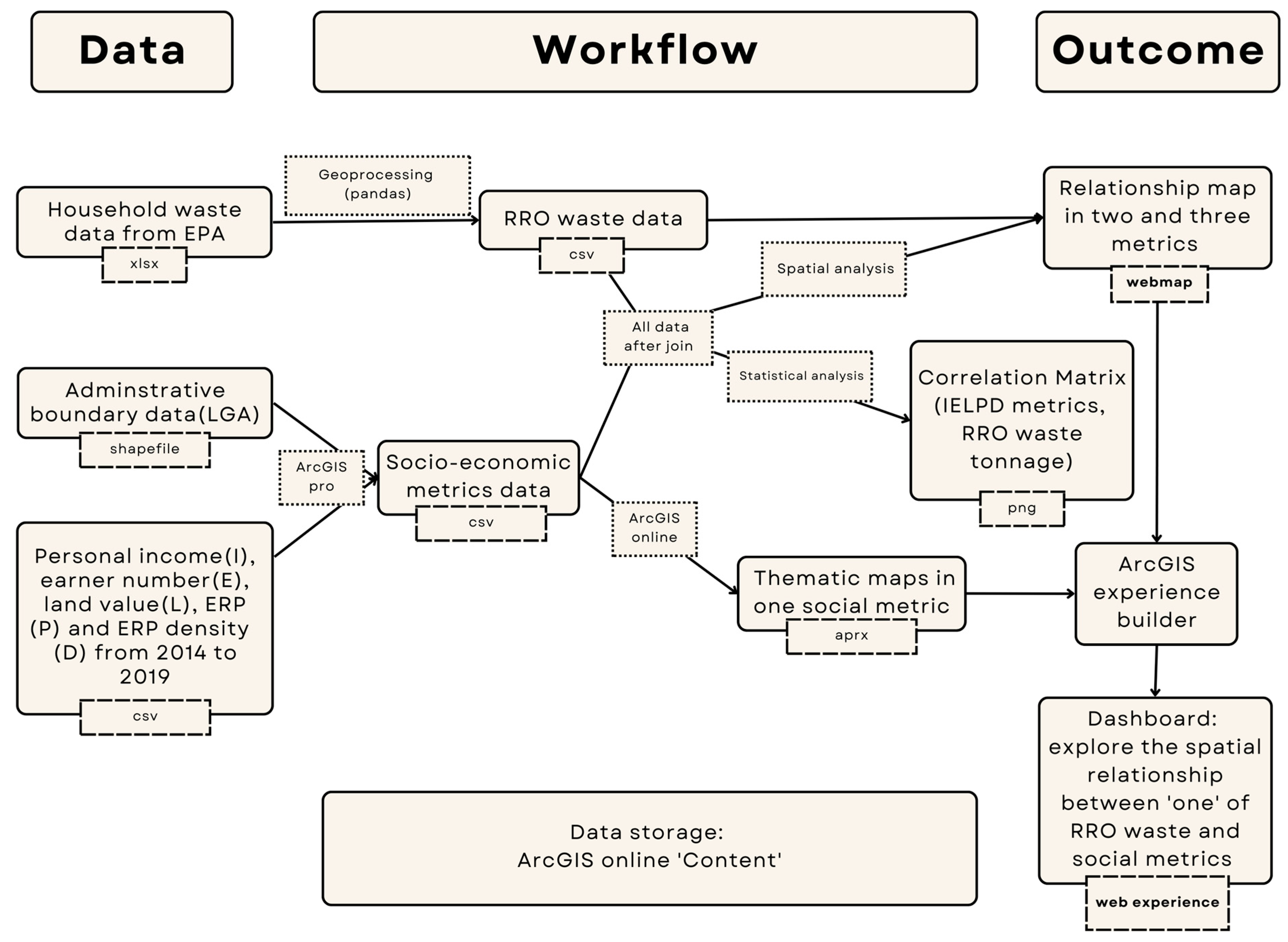
The GIS-based SWVD is developed in this research to provide the possibility of gaining at-a-glance insights from the waste data spatial visualization and relationship analysis across NSW, Australia. Such SWVD provides the possibility of efficient and informed decision-making. Interactive mapping and diagrams in the SWVD show the changing pattern of waste disposal, the relationship map between RRO waste, and population change from IELPD. Moreover, this SWVD makes the outcomes of the research accessible and interactive for the audience, to provide them with the possibility of exploring the needed details further. ESRI products such as ArcGIS Online and experience builder [54] are used to make interactive web maps [55] and dashboards. There is a graph that describes the dashboard development of SWVD in this study (see Figure 4).

4. Results

This section presents the results of the waste data analysis. The results below are organized based on the sequence of the research objectives.

4.1. Spatial Data Visualization of Multiple Metrics

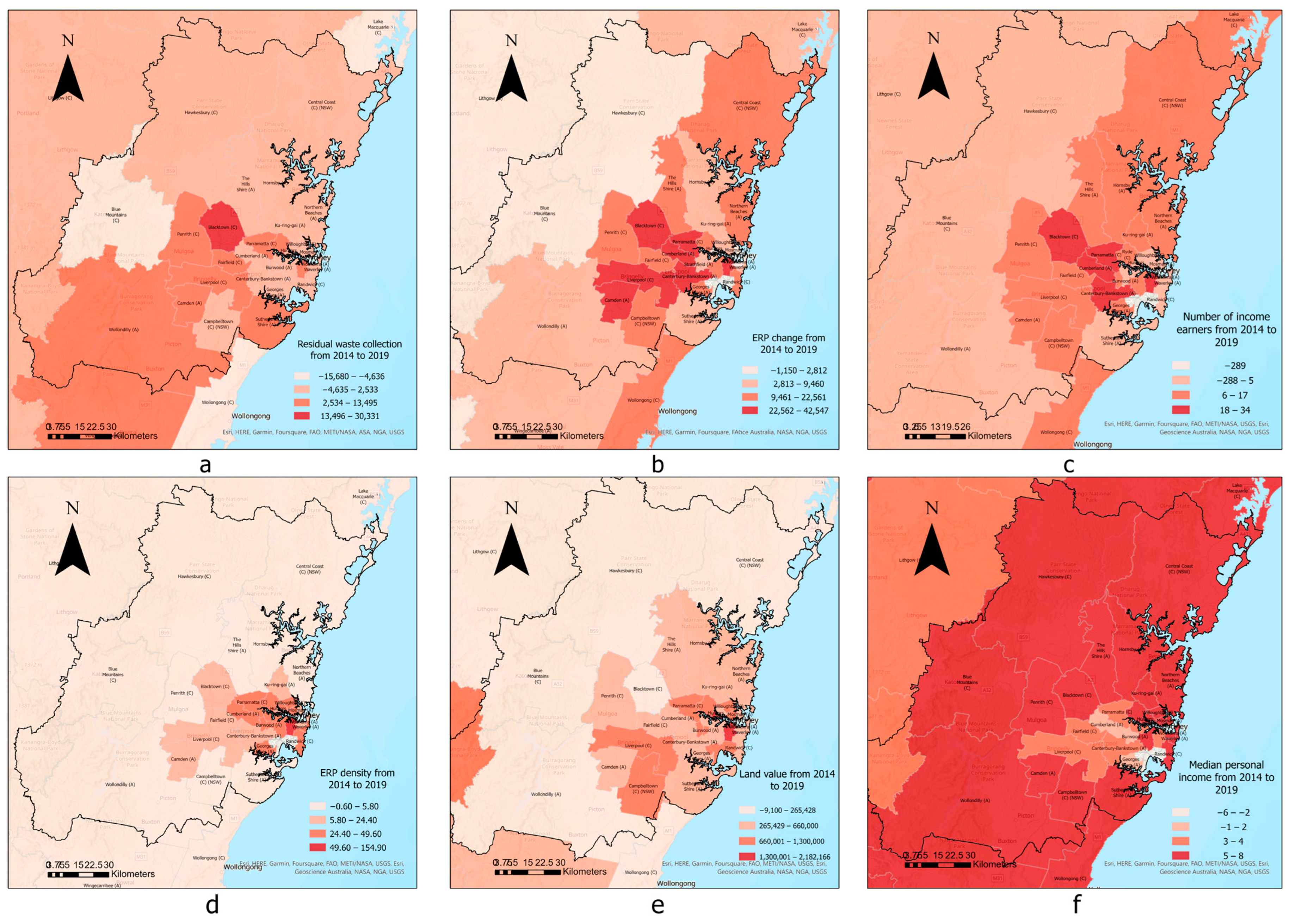
Research objective 1 was to use the RRO stream data after pre-processing to visualize the socio-economic metrics’ datasets for location information, as shown in Figure 5. In Greater Sydney, there are four categories of values identified using the range values of the Jenks Natural Breaks. On the other hand, in the same attribute table, there are RRO waste stream data spanning the years from 2014 to 2019, which can be utilized in mapping the temporal changes between one of the RRO waste categories and social metrics.

Table 4. The thematic mapping of social metrics’ changes in Greater Sydney between 2014 and 2019.

Figure Number/Metrics	Number of Neighbourhoods	The List of LGAs with Special Features
Figure 5a, Residual waste collection	Second shaded: 10	The second top shaded group: Wollondilly, Camden, Liverpool, Penrith, Liverpool, Fairfield, Parramatta, and Ryde, City of Sydney.
Figure 5b ERP changes	Top shaded: 7	Top shaded group: Camden, Liverpool, Canterbury–Bankstown, Cumberland, Blacktown, Parramatta, Sydney.
Figure 5c Number of earners’ change	Top shaded: 4	Top shaded group LGAs: Sydney, Canterbury–Bankstown, Parramatta, and Blacktown.
Figure 5d Population density change (ERP density)	Top shaded: 1 Second shaded: 12	Top shaded: Sydney The second shaded: North Sydney, Burwood, Strathfield, Land Cove, Parramatta, Inner West, Ryde, Canada Bay, Waverley, Cumberland, Willoughby, Randwick.
Figure 5e Land values change	Top shaded: 1	Top shaded group: Sydney
Figure 5f Median personal income change	Top shaded: 22 Second shaded: 2	Top shaded group: Blue Mountains and Hawkesbury, and Wollondilly, Penrith, Blacktown, Camden, Campbelltown, Penrith, Central Coast, and others. The second shaded group: Sydney and Parramatta.

Source: compiled by the author, 2023.

lists various socio-economic metrics and one group of the RRO waste, visualizing the year-to-year unit of income, number of income earners, population, and population density from 2014 to 2019.

The RRO waste tonnage data with respect to residual waste collection were visualized for the Greater Sydney area (see Figure 5a), with Blacktown displaying the most significant positive changes with increasing trends from 2014 to 2019. The representation in the State of NSW reveals that the second shaded centres of residual waste collection are located in LGAs such as Eurobodalla, Shoalhaven, Goulburn, Wingecarribee, Sutherland Shire, and part of the councils of Greater Sydney such as Parramatta, Ryde, the City of Sydney and other LGAs listed in Table 4. The positive changes in the increasing RRO waste tonnage also apply to some of the councils in the north part of the NSW, such as Dungog, Upper Hunter, Coffs Harbour, and Lismore.

Regarding the social metrics, the population changes in the ERP data (see Figure 5b) show that in areas of dotted box such as Camden, Liverpool, Canterbury–Bankstown, Cumberland, Blacktown, Parramatta, and Sydney, the LGAs existed as densely shaded groups with the greatest changes occurring from 2014 to 2019. Once the research focuses on the change in the number of earners (Figure 5c), it becomes clear that there are multiple LGAs in the top shaded LGAs’ list, such as Sydney, Canterbury–Bankstown, Parramatta, and Blacktown.

Referring to the population density changes shown in Figure 5d, there are three categories of values associated with this period. In the top shaded group, only one LGA, the City of Sydney, existed in the group of very high population density changes in Greater Sydney, increasing from 49.6 to 154 ERP/km² between 2014 and 2019. Twelve LGAs are situated in the second shaded group of population density changes around Metropolitan Sydney, displaying increases ranging from 24.4 to 49.6 ERP/km² (see Table 4). The third shaded group is mentioned, with 10 LGAs in underdeveloped areas increasing in density from 5.8 to 24.4 ERP/km².

Meanwhile, the most significant land value changes shown in Figure 5e are in the dotted box including City of Sydney. There are underdeveloped LGAs with the highest increases in median personal income occurring in the dotted box, for instance, the Blue Mountains and Hawkesbury, Wollondilly, Penrith, Blacktown, Camden, Campbelltown, Penrith, Central Coast—Figure 5f. The developed LGAs are in the second-highest category changes (second shaded group) in personal income, such as the City of Sydney and Parramatta.

Through these maps of five years of change in Greater Sydney, Blacktown stands out in the high-frequency list of the top shaded group among social metrics and residual waste tonnage. After mapping one metric, it becomes comparable for researchers to explore the two metrics of land values and ERP in the spatial relationship as shown in Section 4.2 from Figure 6, Figure 7, Figure 8, Figure 9, Figure 10, Figure 11, Figure 12, Figure 13 and Figure 14.

4.2. Spatiotemporal Relationships with Other Metrics

Research objective 2 is to identify the spatial relationships between one socio-economic metric from IELPD, the number of income earners, and the amount of waste generation for the three types of RRO waste. To meet Objective 2, the relationship map and correlation matrices were applied to the RRO data after multiple data pre-processing steps using Python, and the result is demonstrated in Figure 6 and Figure 7a,b with the relationship map across the multiple IELPD metrics. Meanwhile, correlation matrices were able to identify the significance of the correlation between two metrics, especially the waste tonnage, with the other four metrics, as shown in Figure 8a,b for annual data.

Based on the illustrations, the spatial analysis will help to examine the spatiotemporal interaction between household waste tonnage in three channels and other waste disposal datasets in quantile natural breaks. Regression analysis also helps to estimate future waste tonnage in LGAs.

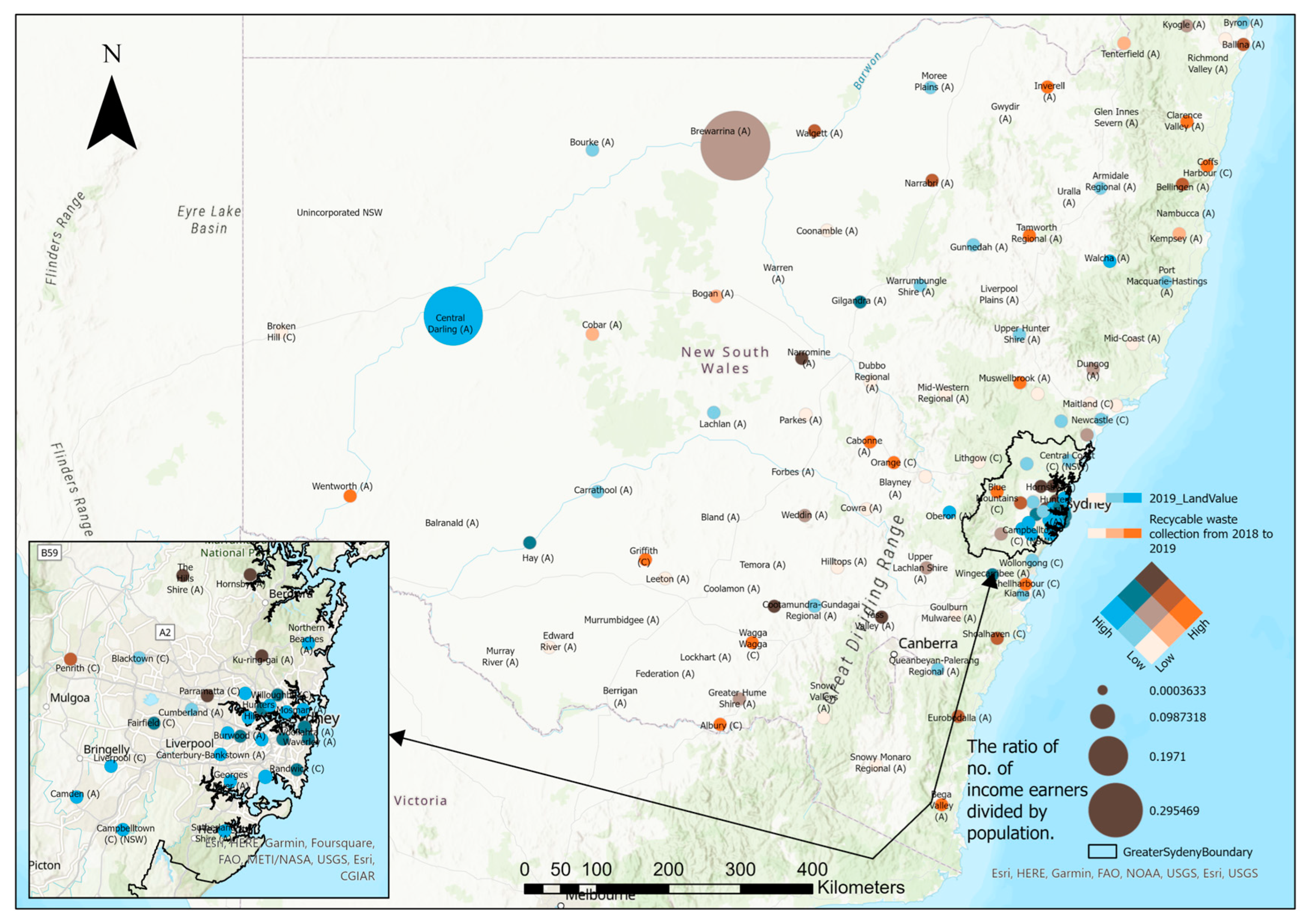
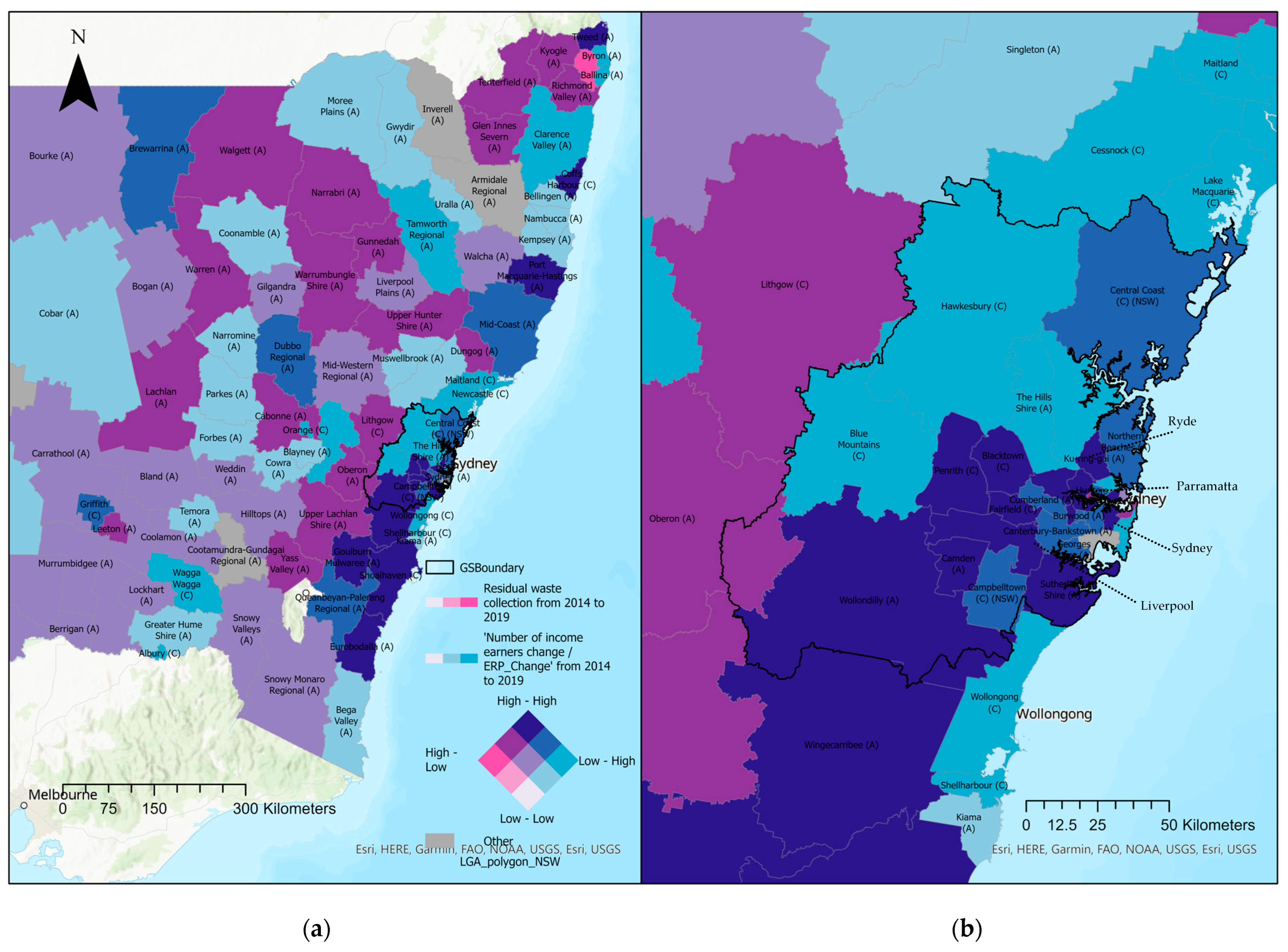
The spatial relationship map in Figure 6 portrays recyclable waste collection and land value. At the same time, the circle size represents the ratio of the number of income earners divided by the population in 2019. Taking the cartographic symbols, a series of LGAs is focused on Greater Sydney, such as the eight LGAs listed in

Table 5. The key LGAs and the special insights in specific figures.

Figure Number	Range/Special Features	Number of Neighbourhoods	LGAs
Figure 6	Greater Sydney/significant ratio of the number of income earners to residents	8 (Greater Sydney) + 2 (Regional NSW)	Greater Sydney: Wingecarribee, Camden, Liverpool, Fairfield, The Hills Shire, Hornsby, Ku-ring-gai, and Ryde Regional NSW: Central Darling and Brewarrina
Figure 7a,b	High-High areas: Significant top-shaded areas, showing a positive correlation with high significance, located in areas among tonnage change in recyclable waste collection and change in number of income earners divided by change in ERP	10 (Greater Sydney) 8 (Regional NSW)	Greater Sydney: Blue Mountains, Blacktown, Parramatta, Strathfield, Sydney, Waverley, Fairfield, Liverpool, Camden, and Sutherland Shire. Regional NSW: Shoalhaven, Bathurst Regional, Lake Macquarie, Newcastle, Port Stephen, Coffs Harbour, Byron, and Tweed.
Figure 8a,b	High-High areas: Significant top shaded areas, positive correlation with high significance located in areas among recyclable waste collection and ERP changes	9 (Greater Sydney) 7 (Regional NSW)	Regional NSW: Shoalhaven, Shellharbour, Port Stephens, Lake Macquarie, Newcastle, Coffs Harbour, and Tweed. Greater Sydney: Sutherland Shire, Liverpool, Camden, Fairfield, Blacktown, Parramatta, Strathfield, Sydney, and Waverley.
Figure 9	A positive correlation between land value, number of income earners and residential waste	6	Parramatta. Ku-ring-gai, Hornsby, Narromine, Junee, Yass Valley
Figure 10a,b	A positive correlation with the ratio among number of income earners and ERP (population) in NSW. Greater Sydney: higher employment rates (number of income earners/population) and high awareness of residual waste behaviour	14 (Greater Sydney) 6 (Regional NSW)	Greater Sydney: Wollondilly, Penrith, Canada Bay, Ryde, North Sydney, Blue Mountains, Blacktown, Parramatta, Strathfield, Sydney, Fairfield, Liverpool, Camden, Sutherland Shire Regional NSW: Eurobodalla, Goulburn Mulwaree, Wingecarribee, Port Macquarie-Hastings, Coffs Harbour, and Tweed;
Figure 11a,b	High-High areas: Significant top shaded areas: positive correlation with high significance located in areas among tonnage change areas among residual waste collection and ERP.	14 (Greater Sydney) 6 (Regional NSW)	Greater Sydney: Wollondilly, Sutherland Shire, Camden, Liverpool, Fairfield, Penrith, Blacktown, Parramatta, Canada Bay, Strathfield, Ryde, Ku-ring-gai, North Sydney, Sydney. Regional NSW: Shoalhaven, Wingecarribee, Port Macquarie, Hastings, Coffs Harbor, and Tweed
Figure 12a,b	Positive correlations with the ratio among the number of income earners and ERP (population)	7 (Greater Sydney) 11 (Regional NSW),	Greater Sydney: Blue Mountains, Penrith, Liverpool, Camden, Sutherland Shire, Parramatta, and Ku-ring-gai. Regional NSW: Albury, Eurobodalla, Wagga Wagga, Griffith, Shellharbour, Bathurst Regional, Cessnock, Lake Macquarie, Maitland, Byron, and Tweed.
Figure 13a,b	High-High areas: Significant top shaded areas, positive correlation with high significance between LGAs with organic waste collection and ERP changes.	6 (Greater Sydney) 3 (Regional NSW)	Greater Sydney areas: Camden, Liverpool, Penrith, Sutherland Shire, Parramatta, and Ku-ring-gai. Regional NSW: Cessnock, Lake Macquarie, and Tweed
Figure 14	The largest recyclable waste tonnage	6	Narromine, Junee, Yass Valley, The Hills Shire, Hornsby, Ku-ring-gai, and Parramatta

Note: High-High areas means positive correlation with high significance among two metrics.

. Moreover, Central Darling and Brewarrina have a particularly significant ratio of earners to residents.

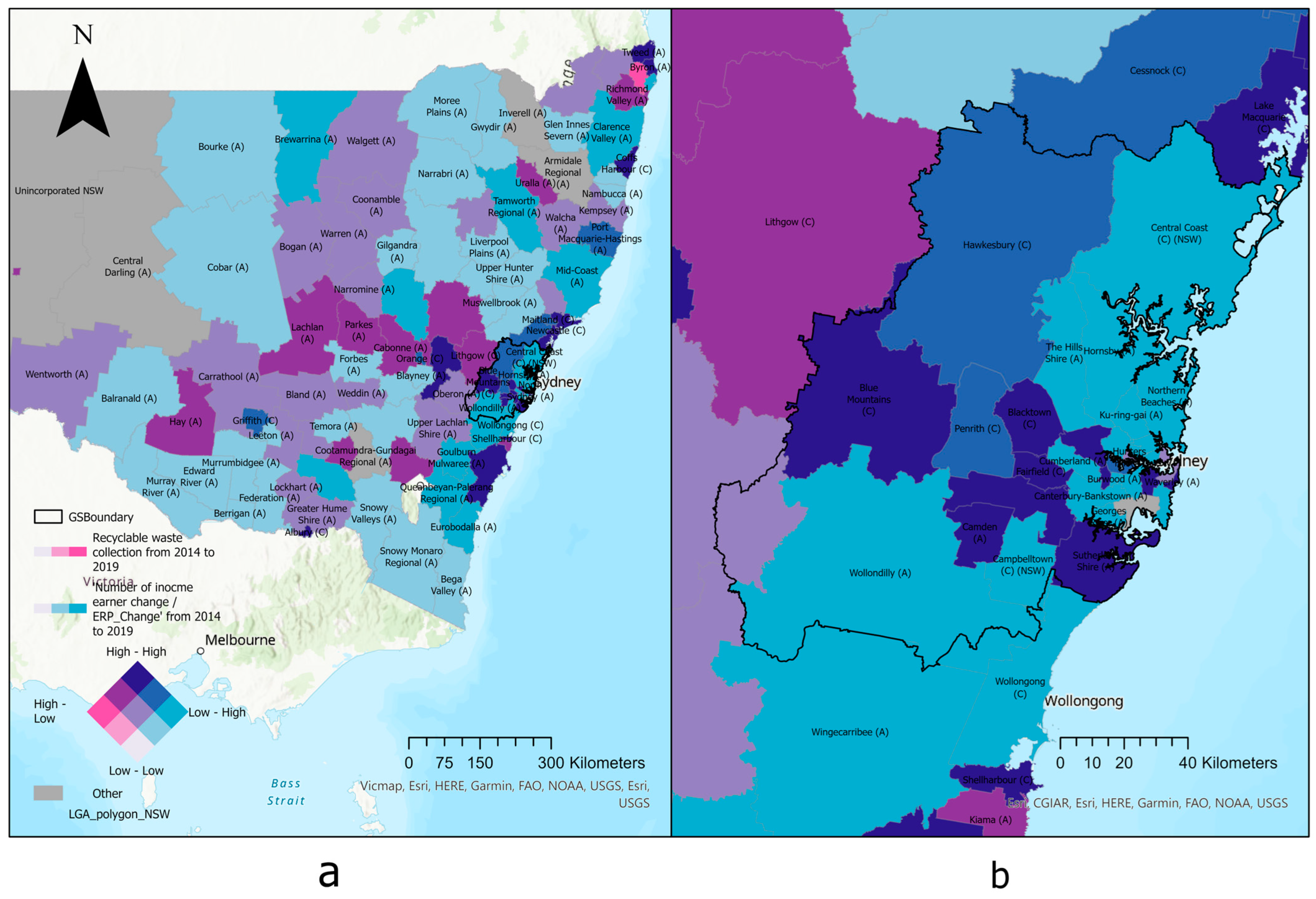
In Figure 7a, there are significant top shaded areas in LGAs which are located in Shoalhaven, Bathurst Regional, and other LGAs in Table 5. These areas display positive correlations between the number of income earners and ERP, which means that there are higher employment rates and increased awareness of recycling behaviours in such LGAs. In Greater Sydney (Figure 7b), there are LGAs such as Parramatta, Strathfield, Sydney, and another eight LGAs listed in Table 5, which also have high employment rates with positive correlations between the change in the number of income earners and ERP changes (Figure 7b). The ratio of the ‘number of income earners’ divided by ERP displayed an increasing trend, which implies an increase in both the employee number and the recyclable waste collection.

Figure 8a illustrates some high-high areas, which are a significant top-shaded group within the Greater Sydney area. The regions are Shoalhaven, Lake Macquarie, Newcastle, Tweed and other LGAs listed in Table 5. In the Greater Sydney area, according to Figure 8b, the relationship map shows high-high areas where there is a positive correlation between recyclable waste collection and population, which includes Strathfield, Sydney, Waverley and other LGAs listed in Table 5. However, there are null values with the new council boundary in the Bayside LGA. Regarding the relationship map displaying ERP density change and recyclable waste collection, the spatial pattern shows the same distribution features as for ERP in Greater Sydney.

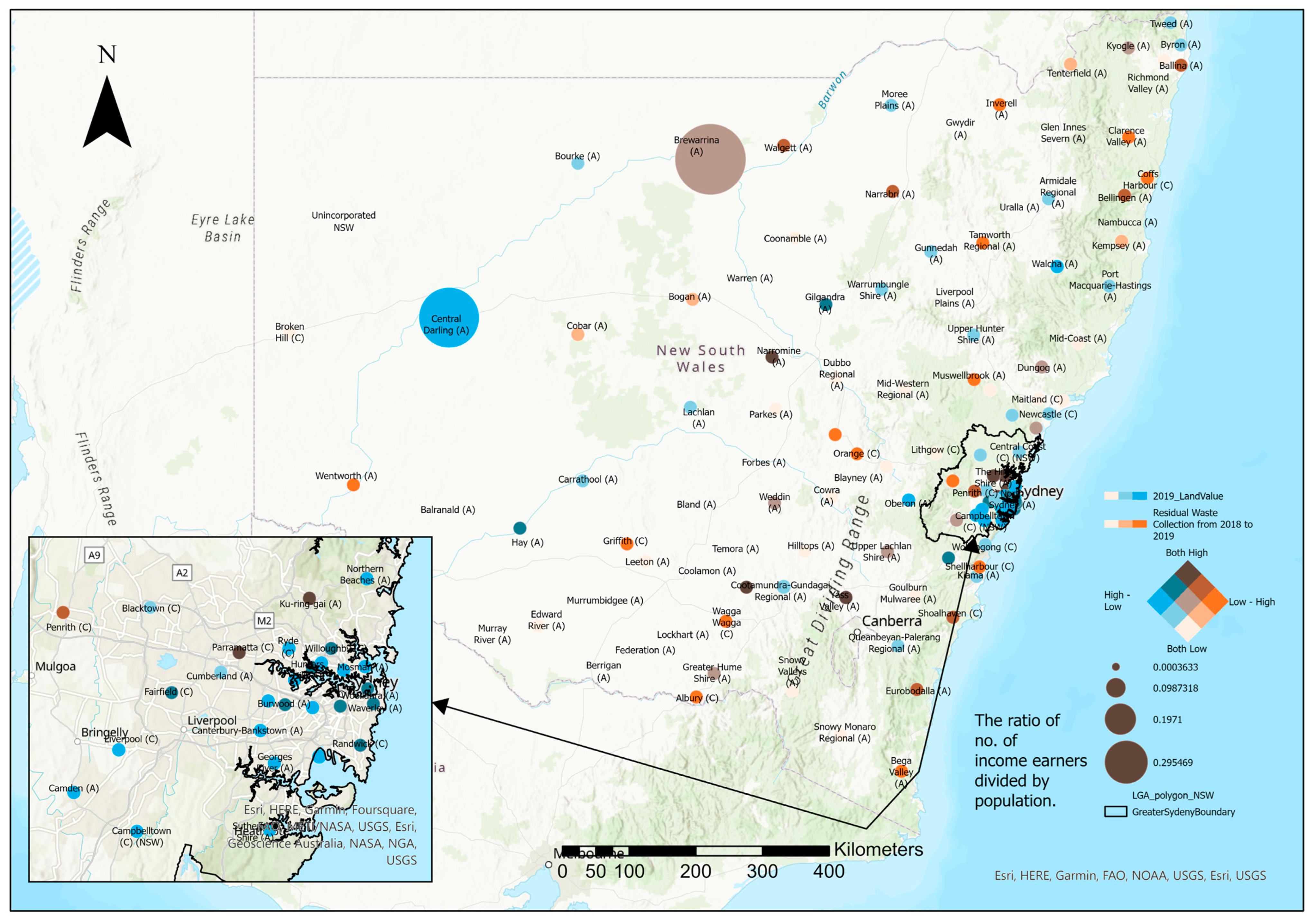
Figure 9 shows the spatial association between residual waste collection and land value, with the ratios between the number of income earners and ERP in 2019. The largest ratio in the chart is in Central Darling and Brewarrina. The diversity in symbology in software needs to be clarified for the districts of LGAs such as Parramatta, Ku-ring-gai, and other LGAs are listed in Table 5. These LGAs have the strongest link between the land value, the number of income earners and residential waste collection.

In Figure 10a at NSW State level, six LGAs, including Eurobodalla, Tweed, and other LGAs listed in Table 5, enjoy positive correlations between the ratio of the number of income earners and ERP. It means there are higher employment rates and high awareness of residual waste behaviour. In the Greater Sydney area, Penrith, Canada Bay, North Sydney, and other LGAs (see Table 5), display the highest ratios between the ‘number of income earners and the change in ERP from 2014 to 2019, with the correlation positive in Figure 10b.

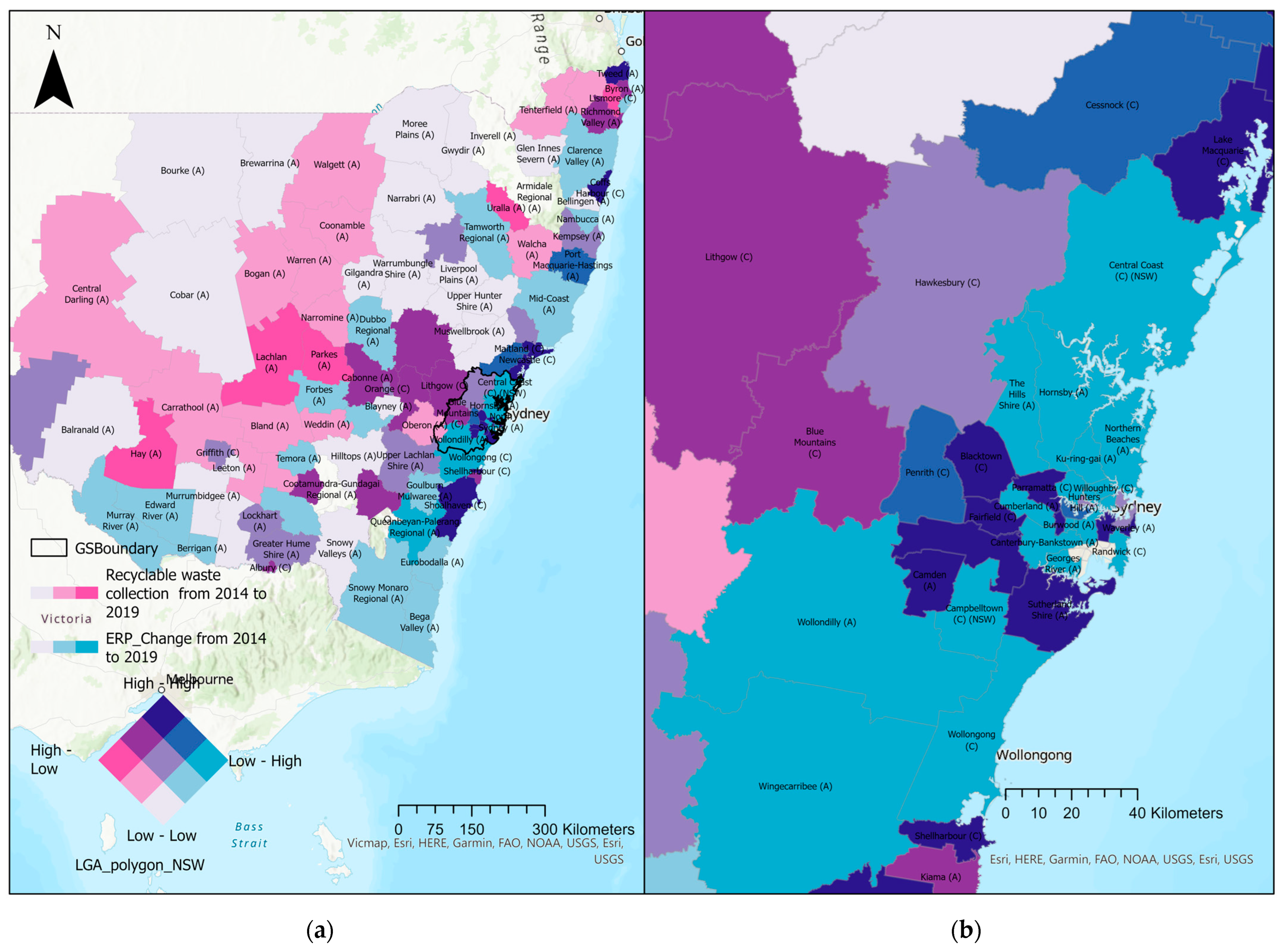
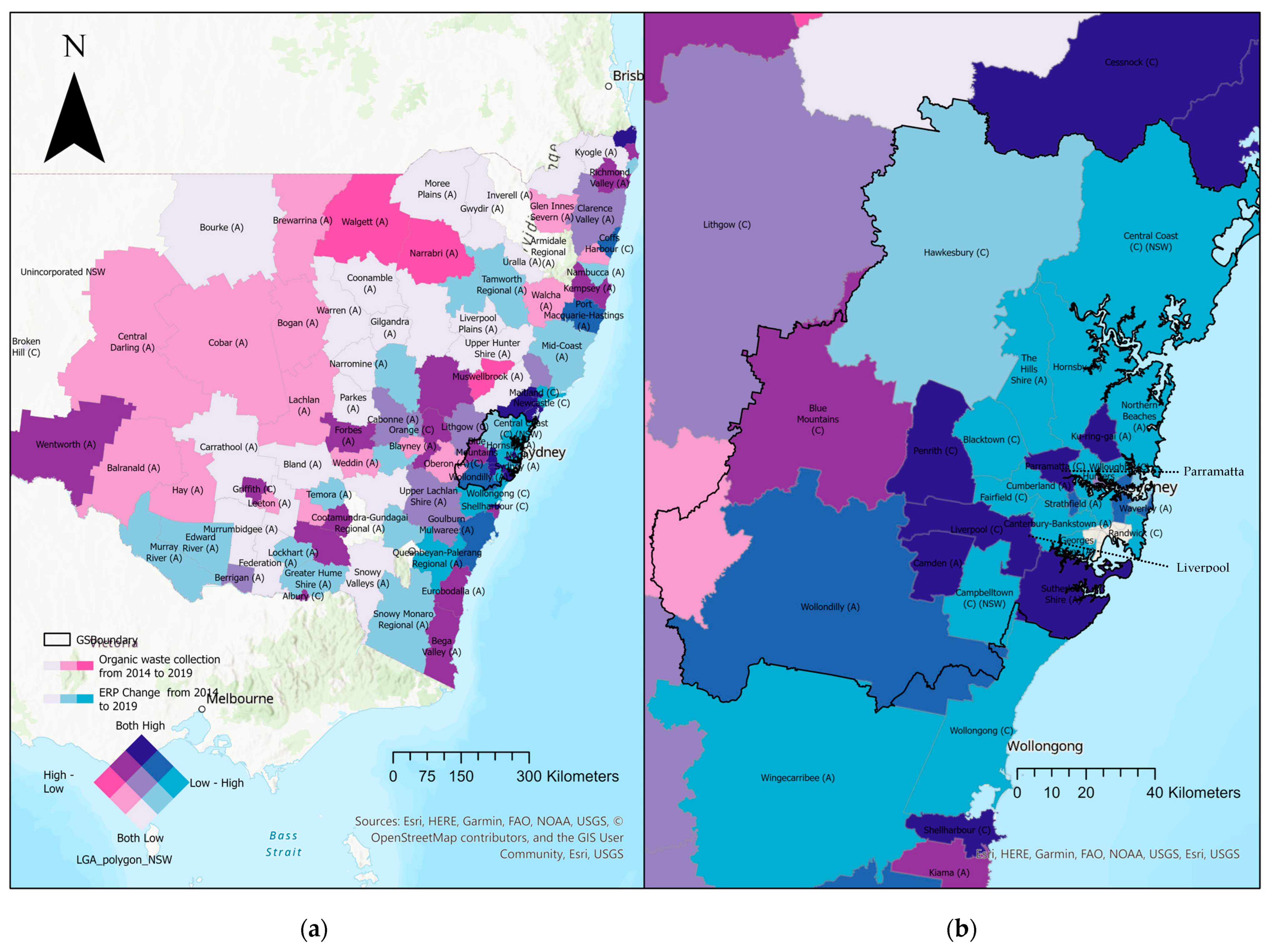
Figure 11a presents significant top-shaded LGAs of residual waste collection (the High-High Areas) and ERP. The LGAs are Ryde, Ku-ring-gai, North Sydney, Sydney and another eight LGAs in Table 5, all located in the Greater Sydney area. In Figure 11b for regional NSW, significant top shaded LGAs (high-high areas) for residual waste collection are Shoalhaven, Port Macquarie, Tweed, and another four LGAs in Table 5. Regarding the relationship map of ERP density change and residual waste collection, the spatial pattern shows the majority of LGAs whose ERP has the high employment rate in Greater Sydney, including Wollondilly, Camden, Liverpool, Penrith, Blacktown, Fairfield and Burwood Ryde, Sydney.

In Figure 12a, there are 11 LGAs, including Lake Macquarie, Maitland, Byron, and another eight LGAs in Table 5. There are positive correlations in these areas between the ratio of the number of income earners and ERP and the waste tonnage of residual waste collection. This suggests that there are higher employment rates and high awareness of organics’ waste disposal behaviour. In Figure 12b, at the NSW state level, there are a number of LGAs, including the Blue Mountains, Penrith, Liverpool, and another seven LGAs in Table 5, which also have the highest employment rates with a positive correlation with the tonnage of residual waste collection.

Figure 13a shows six significant top-shaded LGAs (high-high areas) for organic waste collection and ERP changes, which are Camden, Liverpool, Penrith and another three LGAs listed in Table 5 for the Greater Sydney area. Figure 13b shows additional significant top-shaded LGAs (high-high areas) reflecting the ERP and organic waste collection—Cessnock, Lake Macquarie, and Tweed in regional NSW.

Figure 14 presents the spatial regression between organic waste collection and land value. The circle size reflects the ratios of the number of income earners divided by the 2019 ERP population, including six LGAs listed in Table 5, which generate the largest amount of recyclable waste tonnage. The LGAs in the map’s largest circle differ from those of the others, such as Central Darling and Brewarrina. With respect to the relationship map of the ERP density change and organic waste, the spatial pattern shows the same distribution as that of the ERP in Greater Sydney.

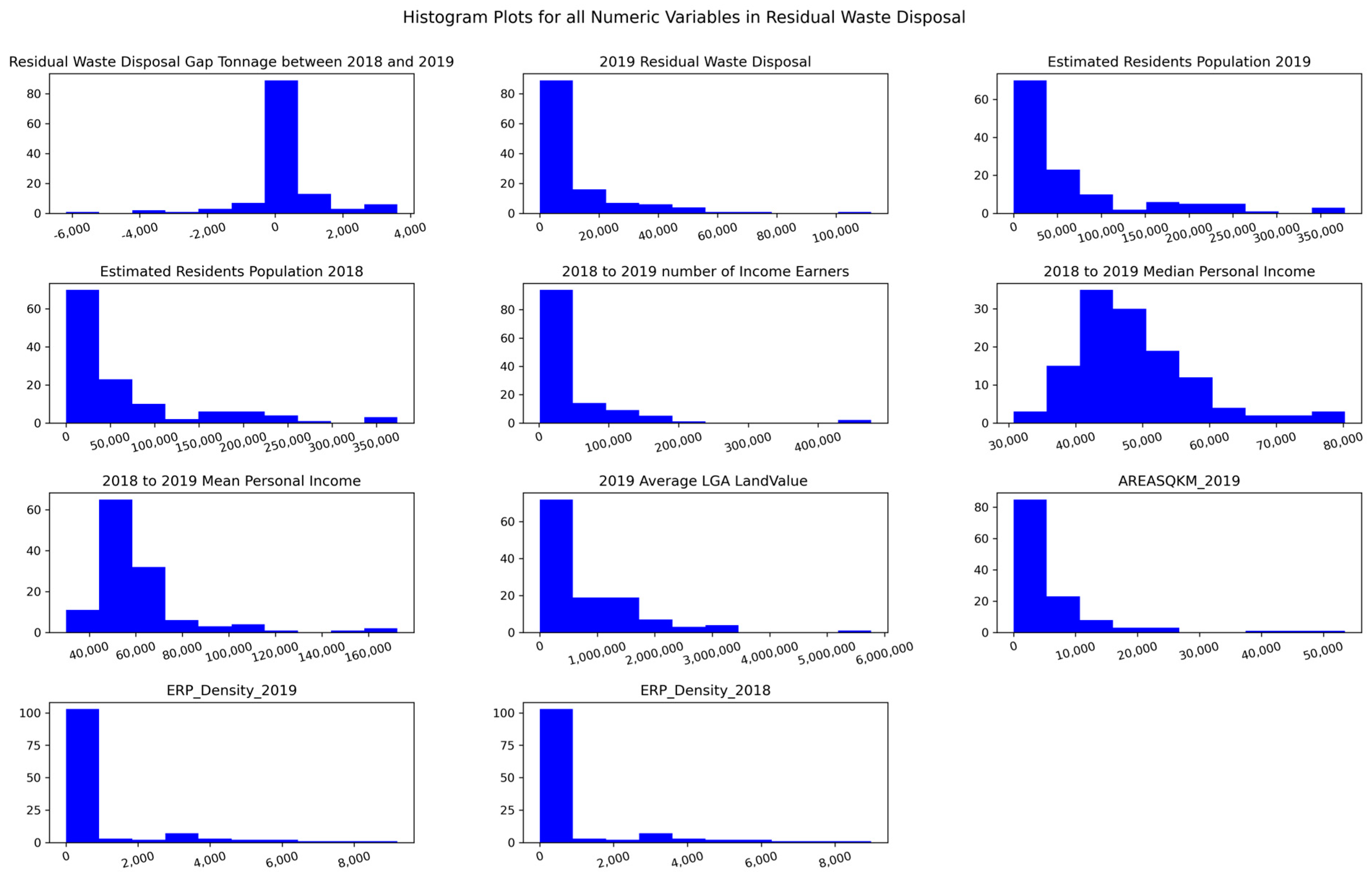
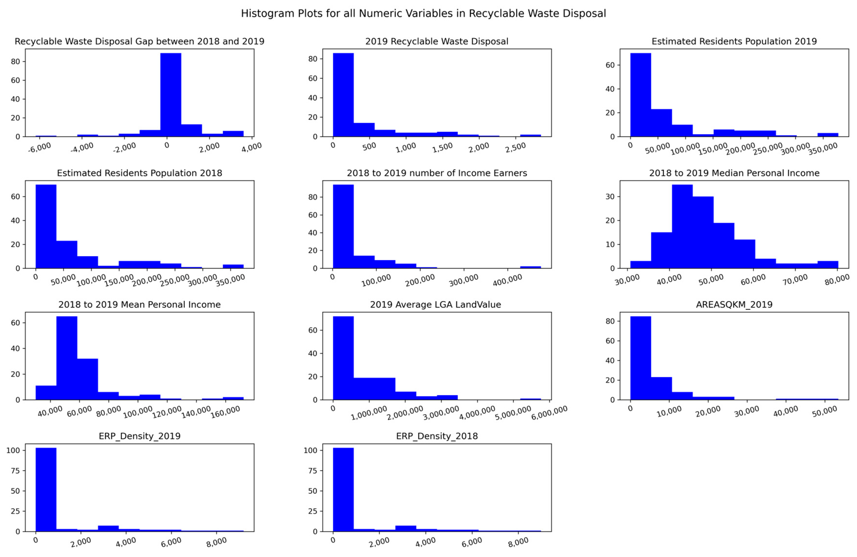
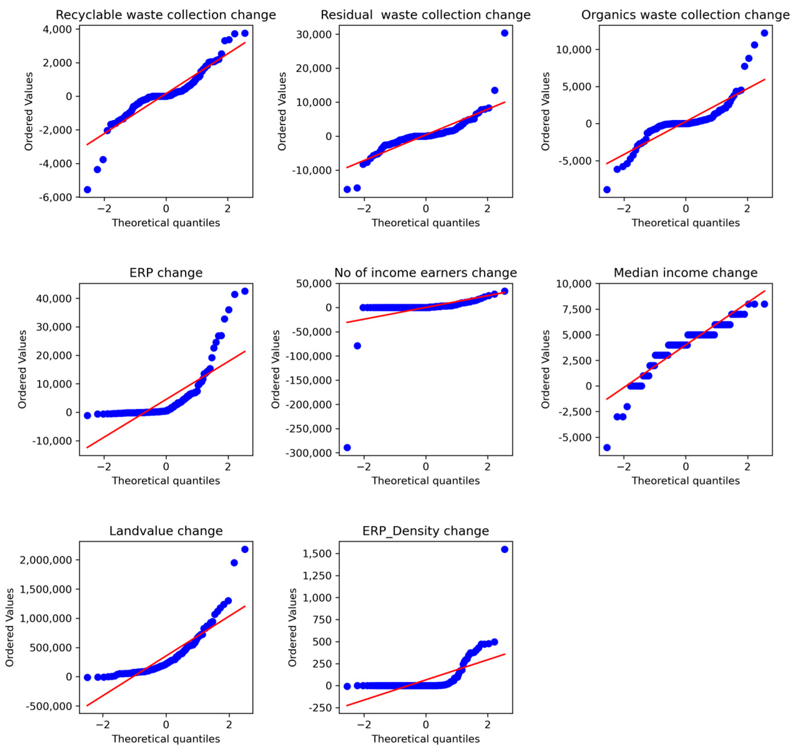
Before the correlation analysis was carried out, the research conducted normality tests on the waste tonnage and socio-economic metrics from Figure 15, Figure 16, Figure 17, Figure 18 and Figure 19. In the Figure 15, this analysis found that land values in Figure 15a and population changes in Figure 15b have lower levels of normalization compared with the consistency of the areas (km²) in the box plot. Moreover, the author investigated that the raw data on the population and land values in NSW from the Australian Bureau of Statistics are not normalized for the multiple LGAs and their different sizes in Figure 18 and Figure 19. Based on the observations of raw data, these inconsistencies in normality are part of the research limitations occurring in these correlations. There are three types of correlation matrix that test the correlation between RRO waste types and the other socio-economic metrics, shown in Figure 20, Figure 21, Figure 22, Figure 23, Figure 24 and Figure 25.

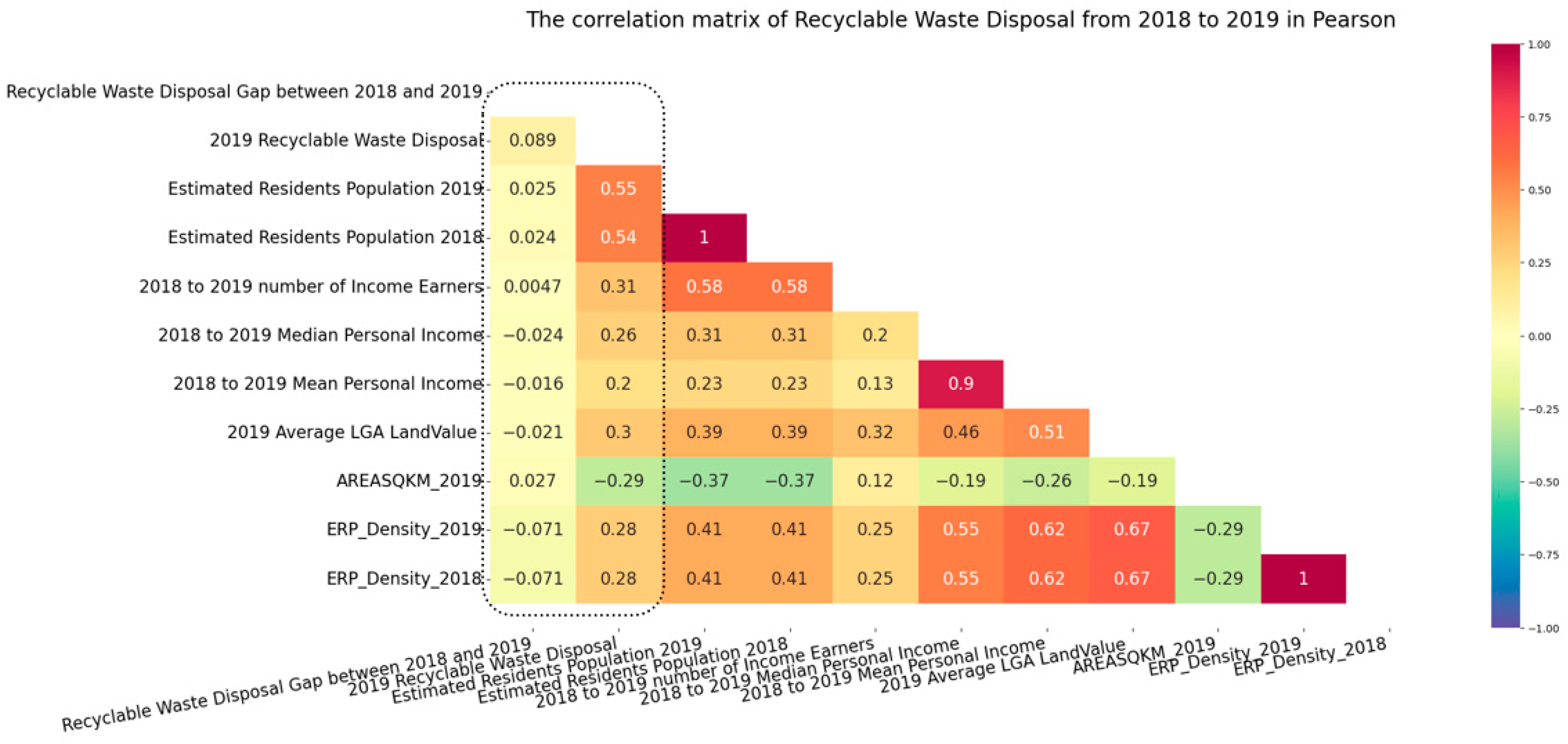
Figure 20 demonstrates the relationships between the 2019’s ERP, the 2018’s ERP, and the 2019’s recyclable waste disposal in Pearson correlation. This figure reveals three correlated factors associated with recyclable waste disposal such as the moderate correlated metric as ERP, and the weak correlated metric land value. In contrast, ERP density and personal income exhibit slight correlated metric s. When considering the supplementary variables, the study finds that the coefficients for the 2019 residual waste disposal and the 2019 average land value in LGAs, are less than 0.5. Furthermore, there is a strong closeness of approximately 0.4 between the 2019 average LGA land value, the 2019 ERP, and the 2018 ERP.

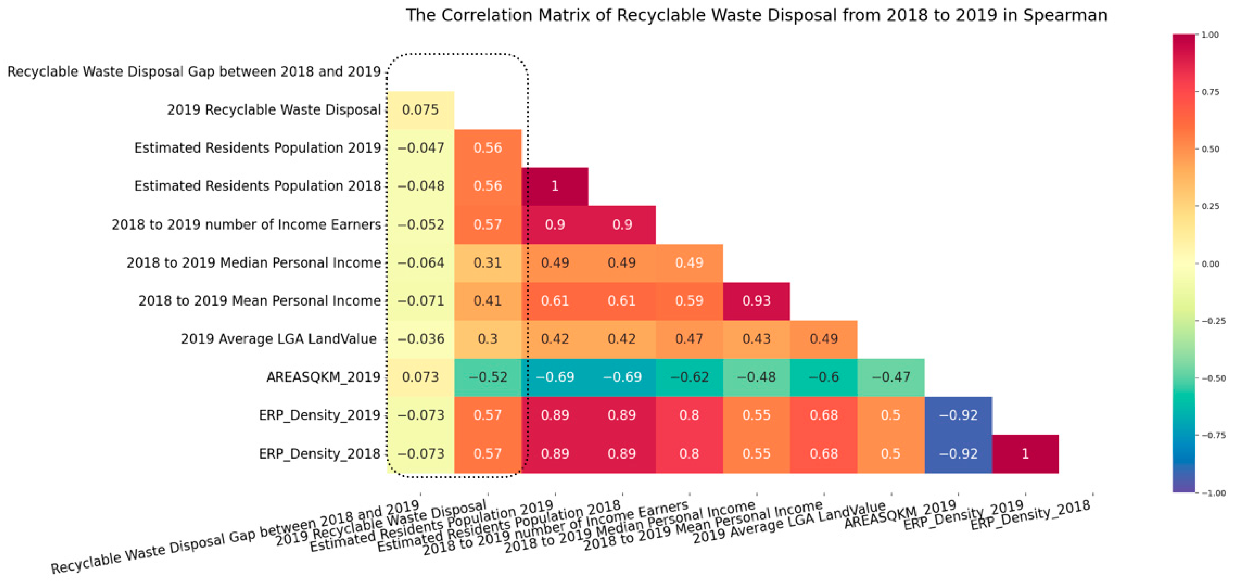
Figure 21 demonstrates the relationships between the 2019’s ERP, the 2018’s ERP, and the 2019’s recyclable waste disposal in Spearman correlation. This figure reveals several moderate coefficient metrics over 0.5 associated with recyclable waste disposal, such as ERP, and mean personal income. Compared to ERP and land values, there are a number of factors with weak correlated metrics, including the number of income earners and ERP density.

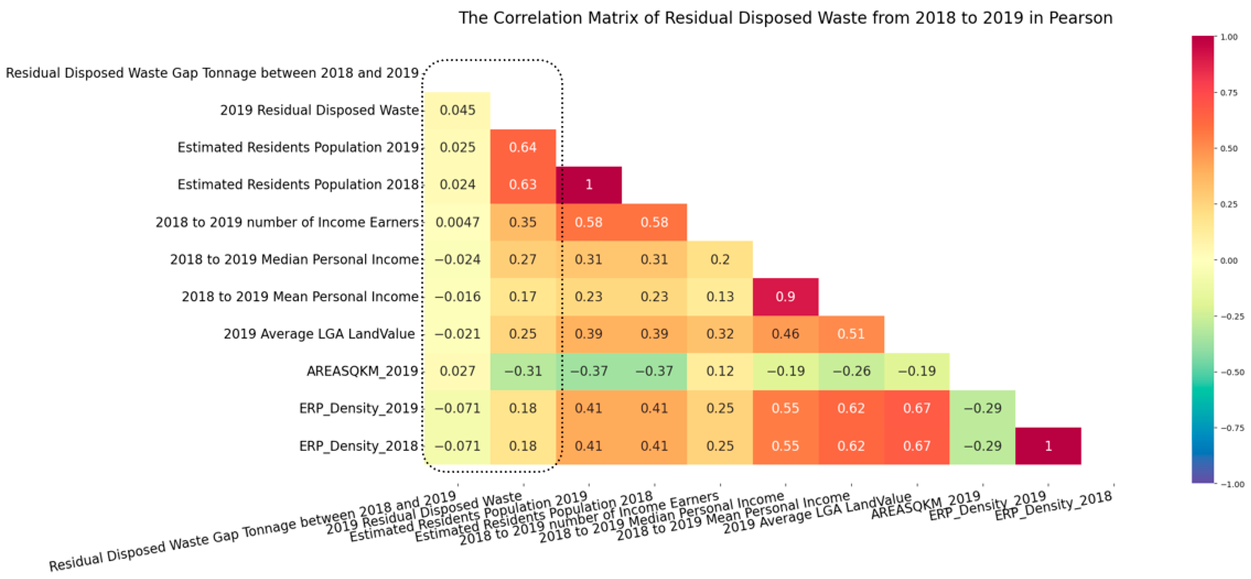
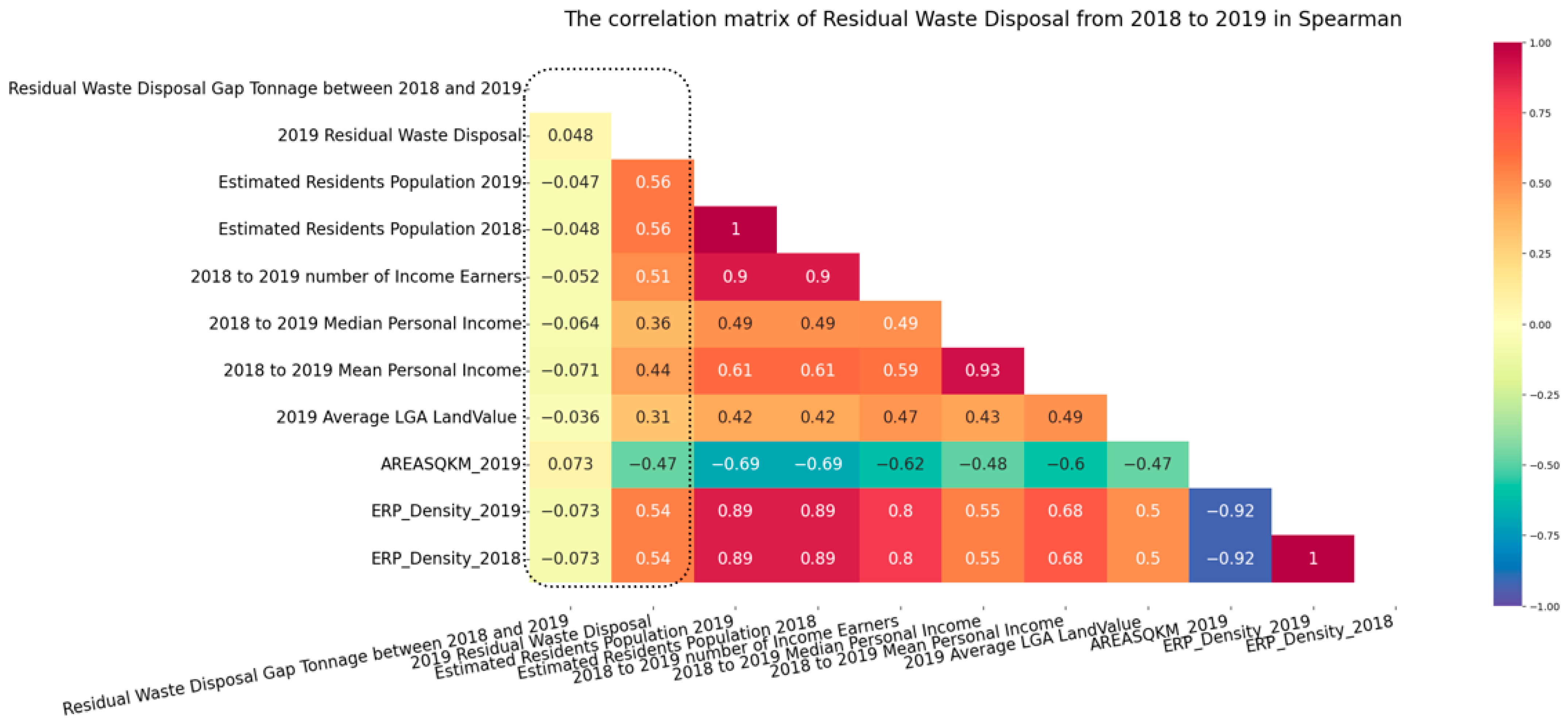
The relationships between the four parameters of interest exhibit stronger correlations in Figure 22 compared to Figure 20 This matrix encompasses residual waste disposal between 2019 and 2018, residual waste disposal 2019, median individual income, and the average land value of each LGA. The correlation between residual waste disposal, and ERP is stronger than that of recyclable waste disposal, indicating that residual waste tonnage increases with population growth. This finding emphasizes the potential for improved recyclable behaviour and reduced residual waste generation in the high land value areas. Importantly, the predicted 2019 resident population demonstrates a moderate positive correlation with 2019 residual waste disposal, offering valuable insight into developing a predictive model for RRO waste.

In Figure 23, the matrix represents the moderate positive correlated metrics over 0.5 between residual waste disposal and ERP, the number of income earners, ERP density, especially the estimated residents’ population in 2019, estimated residents’ population in 2018, the number of income earners from 2018 to 2019, the ERP density in 2019 and the ERP density in 2018. From 0.3 to 0.5, there are multiple weak positive correlated metrics which include ‘2018 to 2019 mean personal income’ and ‘land value’.

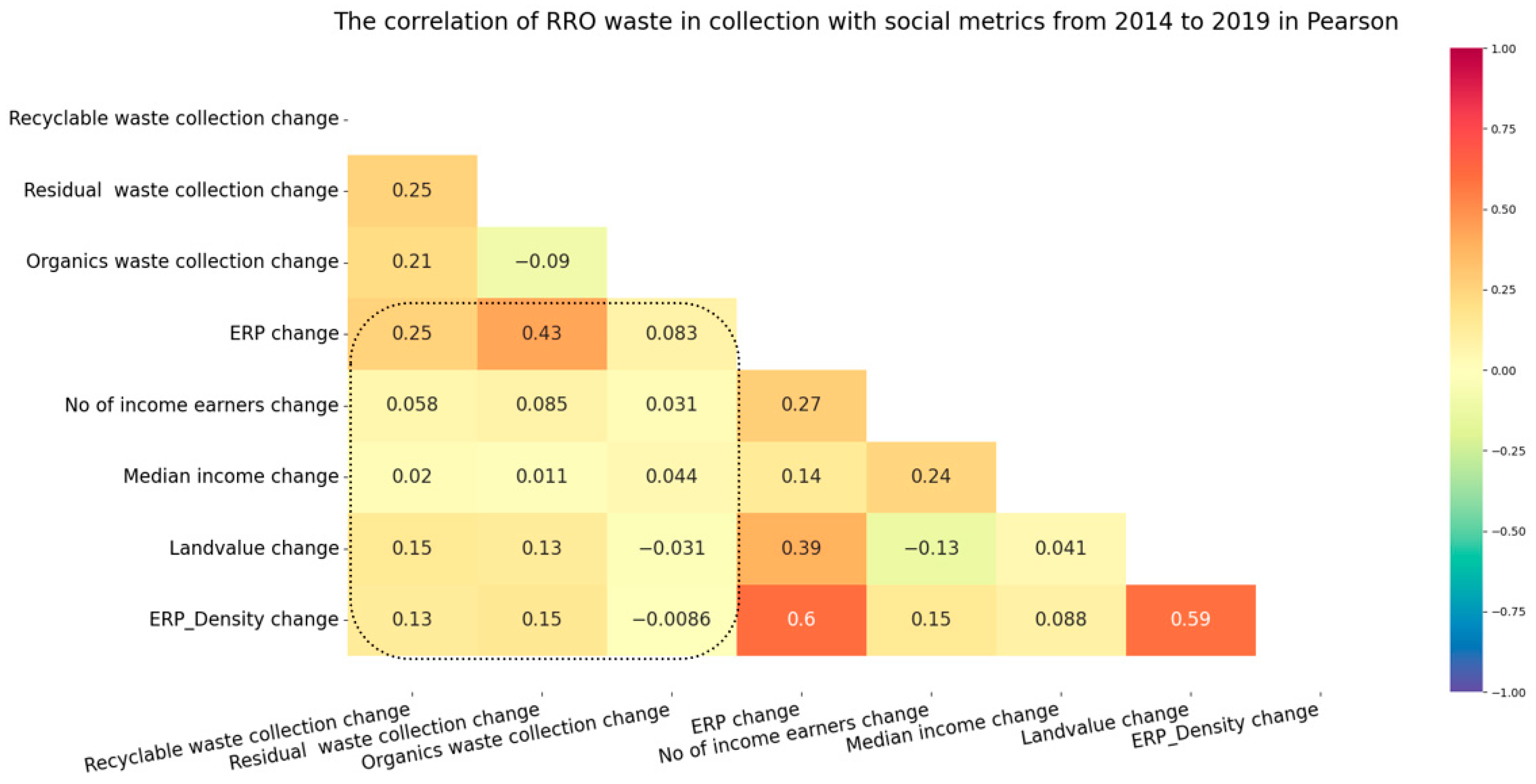
The analysis of recyclable and residual waste disposal from 2018 to 2019 reveals a moderate positive correlation with population and a slightly positive correlation with land values. Concurrently, Figure 24 compares the correlation between the tonnage of RRO waste collection and the change in social metrics. In the correlation analysis of recyclable waste, there are slightly positive correlations for one year, such as 0.25 with ERP change, 0.15 for land value, and 0.13 for ERP density change. However, residual waste displays different weak positive correlations for a single year, including 0.43 for ERP change, 0.13 for land value, and 0.15 for ERP density change. With the similar spatial distribution for land values, ERP, and ERP density changes, waste behaviour varies between recyclable and residual. Recyclable waste behaviour demonstrates a stronger positive correlation with land value than residual waste behaviour.

In contrast, when examining organic waste correlations, the study reveals a slightly positive correlation of 0.083 for ERP, 0.031 for the number of income earners, and 0.044 for personal income. Negative, weak correlations are observed with −0.0086 for ERP density and −0.031 for land values.

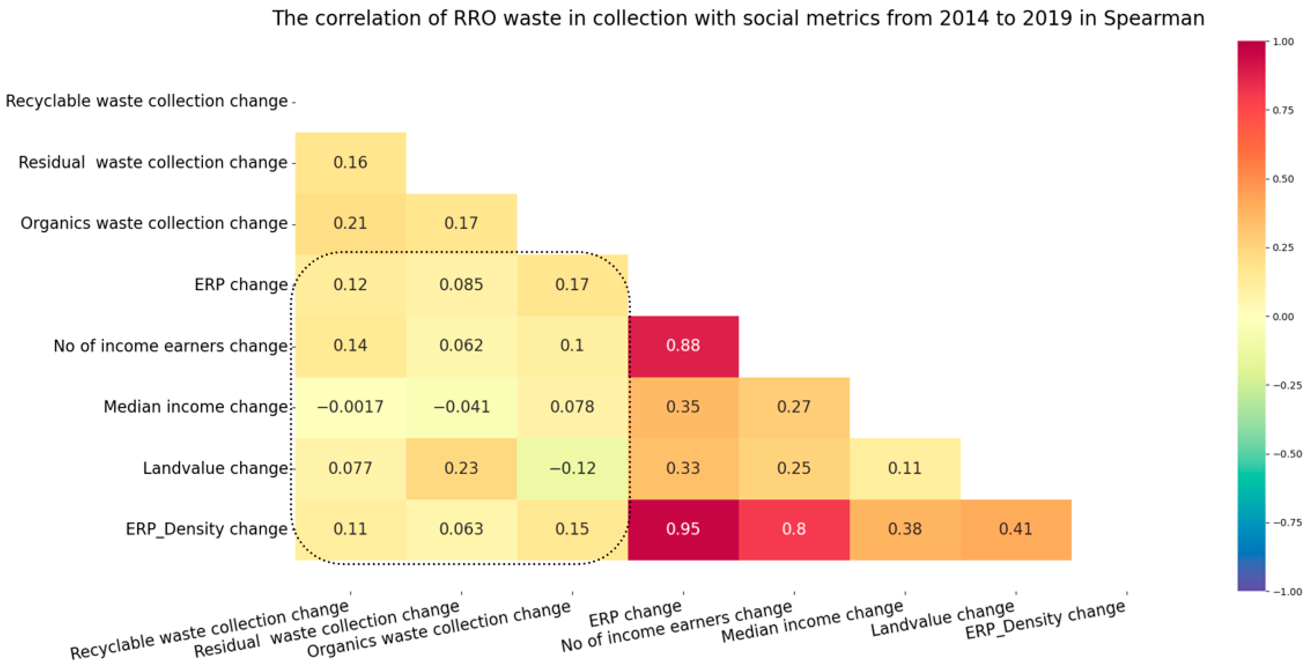
Through the spearman correlation matrix in Figure 25, the correlation coefficient is larger than 0.1, which presents the relationship between recyclable waste collection and no income earners change (0.14), ERP change (0.12). The organic waste collection has similar correlations with the change in the number of income earners (0.1) and ERP change (0.17). However, the correlation coefficient (0.15) between organic waste collection and ERP density is larger than that (0.1) of the number of income earners. In contrast, there are different coefficients between land value and RRO waste collection, especially in residual waste collection; land value has larger correlations with residual waste collection than recyclables collection (0.077) and organics (−0.12).

4.3. Urban Waste Dashboard Development

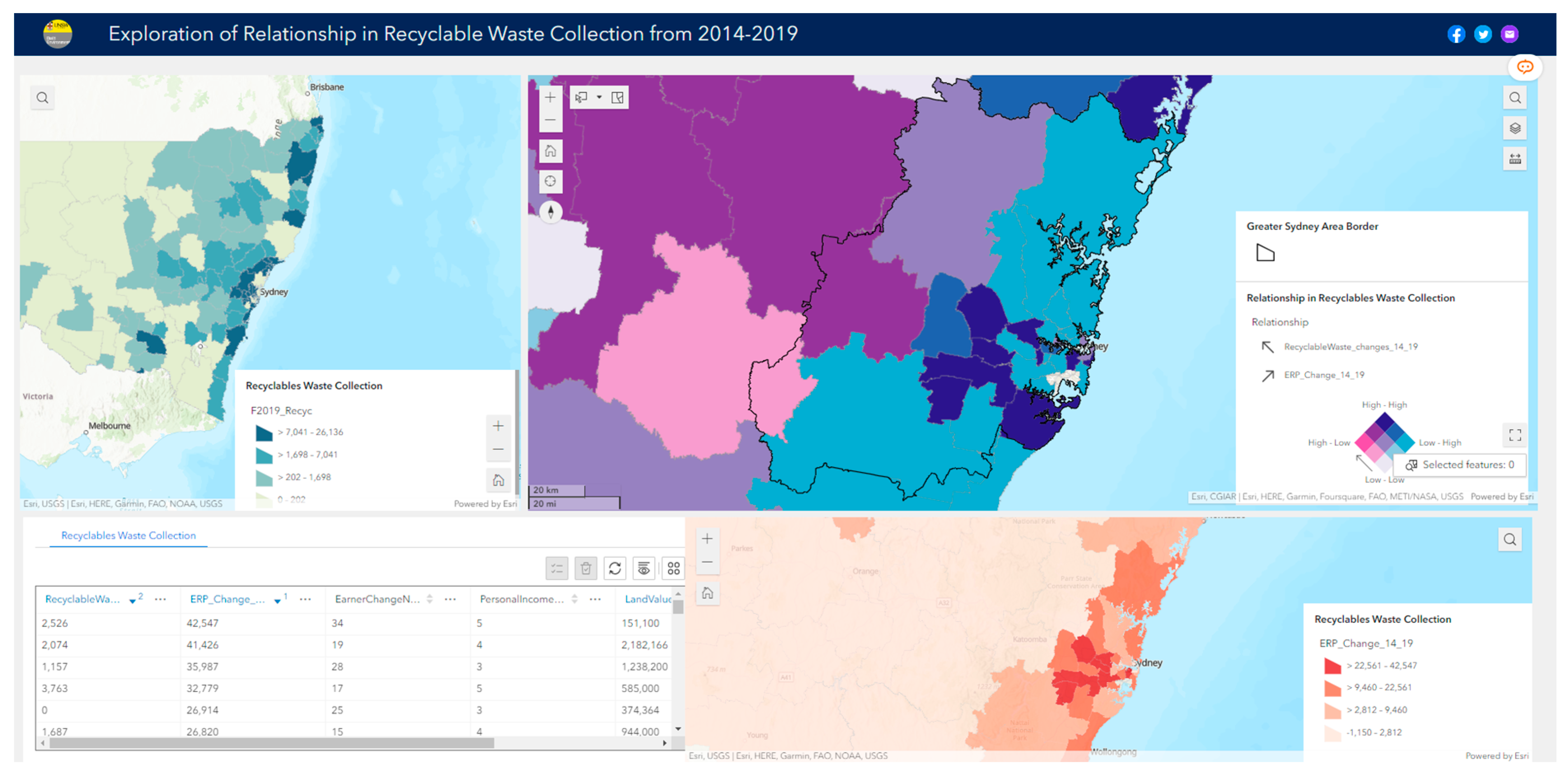
Objective 3 is to develop a SWVD to give insight relevant to the relationship map in waste information. To meet Objective 3, the ArcGIS Experience Builder is applied to geospatial RRO waste data after data storage and visualization steps in ArcGIS Online. The ArcGIS Experience Builder shows the relationship map. The changes between the periods of 2014–2015 and 2018–2019 (see Figure 26) in the spatial pattern of the RRO waste can be easily recognized.

The current phase of the dashboard development entails the implementation of ESRI products to build multiple SWVDs for the three types of waste tonnage data. The RRO waste data visualization at the spatial and temporal level was performed online using the Esri’s ArcGIS Experience Builder platform. It is shown in Figure 26. It reveals the spatial distribution of recyclable waste collection between 2014 and 2019 with the datasets add socio-economic metrics from IELPD. The relationship map only shows the connection between changes in recyclable waste collection and ERP changes between 2014 and 2019. There are other similar tools, such as Experience Builder, which have two other dashboards, such as residual waste and organic waste collection (refer to

Table 6. The related dashboard for the RRO waste collection. Source: compiled by the authors, 2023.

Waste Categories	Material Transferred	Links	Access Date
Residual	Collection	https://arcg.is/0TuWaX	18 April 2023
Recyclable	Collection	https://arcg.is/19vnuf0	30 April 2023
Organics	Collection	https://arcg.is/8b4180	30 April 2023

and

Table 7. The source links are used to produce figures. Source: compiled by the authors.

Figure Number	Source Links
Figure 6	https://arcg.is/1zCPnn
Figure 7	https://arcg.is/1OiqHa
Figure 8	https://arcg.is/0OfDPC
Figure 9	https://arcg.is/1qfHei
Figure 10	https://arcg.is/0P5Drb
Figure 11	https://arcg.is/Srmv4
Figure 12	https://arcg.is/1yWyub
Figure 13	https://arcg.is/1S5eGX
Figure 14	https://arcg.is/00ezO4

) (Figure 26).

5. Discussion

This paper focuses on the explorations of spatial relationships between household waste tonnage and multiple socio-economic metrics. The uniqueness of this study is in the use of the RRO waste data after processing to connect it with the socio-economic metrics in the same dataset. Based on the geographical features, we used the relationship map and correlation matrices to obtain the SWVD, visualize and analyse spatial connections and perform temporal analyses. Rare publications stress the importance of the relationship between waste generation and the IELPD metrics. The development of a SWVD is to provide a visualization platform to display the social-economic connection between RRO waste in urban household waste. Decision-making will be empowered to recognize, monitor, and predict the patterns of RRO waste tonnage with population and land values. Once the waste stream data have open access at a higher resolution than that of the LGA for this study, data analytics tool will be more accurate in portraying spatial relationships to assess the performance indicators for specific waste management [1]. Not only does the RRO waste in high geographical resolution have more geometrics to be considered with respect to local communities, but also, the analytics and visualization of the SWVD play a significant role in predicting waste tonnage and behaviour change [17] for different population sizes and land values.

5.1. Contributions

This paper contributes to the body of the waste management literature by introducing a novel approach to waste data visualization through a methodical analysis and creating a synchronized geographical dashboard. This paper shows how advanced information systems can be utilized for monitoring and screening changes in relationship maps across other metrics. The visualizations can be publicly available to various stakeholders and city decision-makers. With the geographical pattern, household waste in an urban area is divided into the categories of RRO waste into different disposal methods. Thus, a decision maker has access to compare neighbourhood-level variables in IELPD across strategic waste planning.

5.2. Novelty

This study focused on the spatial visualization of the temporal data on the three types of household waste streams to find their geographical relationship for a specific community. This approach is based on a spatial data pre-processing framework to overcome the restrictions of using vector GIS data for spatial visualization. This study focused on the development of a spatial relationship between data exploration and the SWVD, which is a novel practice in the waste management field. As discussed earlier (refer to Section 2), the investigation of spatial area size and spatial distribution is uncommon since there is limited consistency of data collection for locational information for the waste tonnage and socio-economic metrics. However, Python Pandas played a significant role in data pre-processing csv data sources into shapefiles with geographical features, especially the usage of the one-to-many joins. The data sources after pre-processing steps are at various levels in space and time. Regarding space, the multiple social metrics in this study need to use the attribute of LGA to connect each other, and the temporal value needs to calculate the monthly data. Since several data sources from this study have the same two dimensions—space and time—it is feasible for the author to categorize and classify the RRO waste with social metrics into one dataset.

Meanwhile, the RRO waste variations show urban planners how social and economic parameters affect the amount of waste generation across space and time. In recent years, few government reports and limited academic research have considered the relationship between waste generation and socio-economic factors over space and time. They have generally considered the temporal features of the relationship between waste tonnage and other metrics. For instance, from the experimental estimates of waste accounts [56], waste intensity was proposed to estimate the generation of waste per million dollars of value added into the economy and per million dollars of final expenditure of households with time changes.

Consequently, the income of households per capita is a key metric to be considered in waste spatial relationships. The influence of socio-economic factors on household solid waste was noted in Trang, et al. [57], who stressed the statistical significance of monthly household income per capita and educational background. The investigation of data in the study by Trang, et al. [57] was based on a questionnaire of 300 sample households and focused on social and economic factors such as household size, income, education, and environmental concern. In these metrics, the temporal variation of income is the key part, together with the spatial distribution.

Previous studies examining the relationship between waste generation and socio-economic metrics have been limited to small-area predictions, waste estimations, and geospatial dashboard development. In one such study, Kontokosta, et al. [23] used a socio-spatial model to estimate municipal solid waste (MSW) based on demographic and socio-economic factors, including racial percentage, employment, education, elderly population, household type, rent, and income. This study found that demographic variables were highly significant predictors of MSW generation but did not explore the spatial relationship between waste generation and socio-economic factors. In another study, Madden, et al. [58] used GIS to estimate household waste based on dwelling type and waste type (residual fraction, dry recyclables, and garden waste). Additionally, a study by Delaney, et al. [59] developed a geospatial dashboard to monitor wind turbine blade waste at the end-of-life stage, identifying a significant spatial relationship between blade waste weight and turbine power rating. However, this dashboard primarily focused on data tracking rather than analysing waste data variation at the spatiotemporal level.

The present paper also addresses the gap of waste management by providing a unique SWVD for waste authorities to examine spatial relationships in LGAs. GIS and spatial visualization work as mapping tools and deliver a pathway to analyse spatial relationships and interactively display them on a webpage.

5.3. Specific Findings

The first research objective visualized how RRO waste has changed in the specific local community over time at the LGA level. The visualization shows waste disposal in collection, disposal, and recycling pathways from 2014 through 2019 in space and time. Separate spatial distribution maps were developed to depict the spatial relationships among land values, number of income earners, household income, and ERP. The three-path analysis compared 109 LGAs between 2014 and 2019. In these research objectives, the mapping of data after mass data preparation may be identified in the current results. This innovative approach to visualizing RRO waste distinguishes differences over time in multiple jurisdictions. However, the availability and resolutions of time series datasets from waste authorities hampered previous investigations in this case. There are LGA level datasets which were studied. The data visualization of waste-related social metrics can provide waste authorities with significant insights into annual changes, and regional NSW’s economic development can be identified through household income and environmental consciousness.

The second research objective in Table 3 explored the links between neighbourhood social-economic characteristics and the RRO waste tonnage, especially the utilization and distribution over time and location. This objective was achieved by exploring the spatial relationship between the metrics of IEPLD from 2014 to 2019 (refer to Section 4.2). Regression can help to analyse neighbourhood-level correlations for several factors. The spatial and temporal analysis in ArcGIS Pro benefits from neighbourhood relationships. Pearson’s and Spearman regression was utilized to increase the regression’s interpretability for multiple socio-economic components, including the IELPD metrics. These findings indicate that organic waste is collected more in rural areas, which have lower population density and low land values, while urban areas exhibit a reduced likelihood of organic waste collection.

The third research objective evaluates the spatial relationships for, population, and RRO waste tonnage, the year-to-year changes of IELPD in 5 years differently from a connective dashboard.

The third research objective, what type of SWVD should be developed to better depict and include the spatial relationship with other metrics from waste stream data, was addressed by uploading pre-processed datasets onto an online platform that includes an interactive dashboard. After saving pre-processed datasets, users can search for five years of EPA waste data. This study’s SWVD enables users to analyse raw data pre-processing and data transformation for waste data management. For example, the SWVD in ArcGIS Experience Builders in ESRI, involves interactive visualizations about current versions of dashboard, such as recyclable waste collection in 2014, recyclable waste collection in 2019, and LGA population in 2020.

5.4. Value of the Findings

When the complete dashboard is clicked on a spatial map, waste tonnage information appears on an interactive web page, along with local government statistics. The current edition will bring more social and economic datasets to the same polygon and model. It will enable the public and decision-makers to access waste management matters. These dashboards provide historical spatial data visualization of the waste stream for accessible datasets and a digital tool to examine present spatial relationships at the neighbourhood level. The findings of this study enable decision-makers to recognize waste data trends and impact variables over the years in an interactive dashboard that presents the three waste data categories, with a valuable geographical relationship at the neighbourhood level. It would expand the geographical understanding of socio-economic parameters and waste streams. The SWVD utilized a relationship map in ArcGIS Experience Builder in this research. The neighbourhood analytics in the household waste stream play a significant role in performance assessment for urban metabolism [8] and carbon reduction [17], specifically the identification and monitoring of potential human-centric factors connected with waste generation.

5.5. Practical and Theoretical Implications of the Study

The SWVD established in this research are important for waste management. For instance, radio frequency identification (RFID) technology is often utilized in monitoring waste bins, and the dashboard of waste RFID provides a real-time track for household waste in the literature [60]. Meanwhile, the findings of this study in dashboard development empowered historical data insights into, the tonnage of RRO waste collection, and the spatial relationships with the IELPD metrics from 2014 to 2019 in financial years. The digital transformation in waste data visualizations is shown with spatial analysis and a digital tool developed to enable decision-makers to monitor and evaluate data trends using a dashboard. The authorities can easily compare neighbourhood-level variables relevant to strategic waste planning with appropriate criteria or metrics aligned with the SDG goals. In urban waste, the optimization of waste transport networks and the selection of waste facility sites can be adjusted and assessed with historical waste stream trends and real-time monitoring. For instance, realigning the spatial distribution of one of RRO waste through the differentiation of population and land values. Hence, waste management will be empowered with multiple dashboard development and spatiotemporal analysis to support communities to achieve increases in the quantities of recyclable waste and reduction in residual waste, to enable carbon reduction in residuals and advance circular economy principles. As mentioned in a study conducted in Iran, the researchers [61] proposed an assessment framework with factor analysis involving 60 social, economic, and environmental indicators to assess sustainable development. It stresses the importance of factor analysis in waste disposal involving the ‘sustainable development goals’ (SDGs) and government bodies. Similar to SWVD, the spatial analysis visualization of historical trends would contribute to waste transport and facility site selection. In waste generation and management, highly efficient waste management supports SDG 06—‘clean water and sanitation’—with less underground pollution, and the neighbourhood analytics in waste generation stress the importance of SDG 08—‘decent work and economic growth’—especially in land values and population growth. This two highlighted sustainable development goals reflect the importance for waste generation of these spatial relationships around waste streams in communities.

5.6. Future Research Directions

This project transforms accessible datasets into interactive diagrams illustrating historical spatial and temporal data. Digital transformation for waste management is still in progress for long-term analytics, and waste stream data collection is a data governance challenge. With decades of data on the waste stream in developing countries, assessing waste impact from a social, economic, and environmental viewpoint is very significant.

In these research topics, when industrial partitioners can have relationship maps and spatial data visualization multiple waste streams can be seen in and support smart waste management. The key challenges of digital waste management include extracting and transposing datasets from *.csv formats and text-based annual reports for data processing, geocoding, and visualization in GIS. Future studies should empower and model waste stream optimization through trend analysis with spatiotemporal data visualization, even short-term prediction analytics in the waste stream through machine learning at the neighbourhood level.

6. Conclusions

This paper aimed to address the gap in developing an innovative visualization for analysing household waste tonnage related to known social-economic metrics over space and time. The paper demonstrated how methodical data pre-processing could be used for visualizing the relationship among several variables affecting the amount of waste generated over the years. The analytical tool was supported by a large dataset of original data, including the RRO waste tonnages and various variables, such as the metrics from IELPD. The variables were examined to connect the socio-economic metrics in local government areas. The paper contributes to the body of knowledge by developing and utilizing an innovative method in waste management for spatial relationship maps that is critical information for monitoring waste tonnage and potential socio-economic factors in local communities over the years.

The results of the present exploratory investigation, through extensive data pre-processing of urban waste, demonstrate areas with a high correlation between RRO waste and social metrics in the selected LGAs around NSW’s regions.

6.1. Relationship Map and Correlation Analysis

Through the annual and three-year gap data, this study uses ESRI to generate a relationship map with RRO waste tonnage, land value, personal income, the ratio among earner numbers, ERP, and ERP density. The relationship map reveals the four metrics’ locational information through spatial visualization, which makes a great difference by supporting the decision-maker with insights. Meanwhile, with the implementation of Pearson correlation, the outcome of the correlation matrix indicates the potential relationship between two metrics, providing a background of correlation within this study.

The spatial relationships in the map and regression analysis provide a potential solution about disadvantaged areas and whether they have any comparison to high-density CBD areas, especially regarding residual and recyclable waste. These outcomes can be considered for strategic planning to decrease the tonnage of household waste in local government areas, especially improving the percentage of recyclable waste in household waste. According to the outcome of the analysis, the main highly correlated parameter is ERP compared to other metrics, with a weak correlation in recyclable and residual waste. For instance, land value is more significant than personal income for recyclable and residual waste tonnage. On the other hand, population and land values were stressed as important in relation to recyclable and residual waste generation.

6.2. Dashboard Development

Through the ecosystem of ESRI, this study works through data pre-processing in ArcGIS Pro and Python, finalizing the accessible datasets from the raw datasets of waste authorities. Moreover, ArcGIS Online played a significant role in storing spatial datasets as a cloud-based mapping tool. All the analysis in this tool can be imported into ArcGIS Experience Builder for interactive visualization with relationship maps as one SWVD.

In the meantime, a smart waste interactive dashboard was developed with a spatial relationship embracing waste data trends from 2014/2015 to 2019/2020. Furthermore, the selected IELPD metrics are land value, earner number, personal income, and population in regional areas. In the dashboard, there is a data table that includes these metrics variation from 2014 to 2019. In addition, there is a significant metric for ERP relationship map with RRO waste collection.

This research paper provides valuable insight for waste practitioners and urban planners to recognize the GIS-based relationship based on the local community at the social and economic level, especially population development, land value, and housing. Above all, the value of the presented methodology for cross-spatial visualization and SWVD development is that the regional development in household waste plays a significant part in catering to Net Zero plan [62], especially optimizing the ratios of organics waste. It will support decision-makers in achieving this initiative’s target, especially in reducing carbon emissions step by step.

References

1. Ferreira, D.C.; Caldas, P.; Varela, M.; Marques, R.C. A geometric aggregation of performance indicators considering regulatory constraints: An application to the urban solid waste management. Expert Syst. Appl. 2023, 218, 119540. [Google Scholar] [CrossRef]
2. Liao, N.; Lü, F.; Zhang, H.; He, P. Life cycle assessment of waste management in rural areas in the transition period from mixed collection to source-separation. Waste Manag. 2023, 158, 57–65. [Google Scholar] [CrossRef] [PubMed]
3. Kaza, S.; Yao, L.C.; Bhada-Tata, P.; Van Woerden, F. What a Waste 2.0: A Global Snapshot of Solid Waste Management to 2050; World Bank, Urban Development: Washington, DC, USA, 2018. [Google Scholar]
4. WHO. Sanitation. Available online: https://www.who.int/news-room/fact-sheets/detail/sanitation (accessed on 27 April 2023).
5. Rachal, M. Latest UN Climate Change Report Highlights Urban Mitigation Strategies, Circular Materials Management. SMARTCITIESDIVE. 2022. Available online: https://www.wastedive.com/news/ipcc-climate-mitigation-report-circular-materials-management/621649/ (accessed on 8 April 2021).
6. Webster, K. Learning Path. The Circular Economy in Detail; Ellen Macarthur Foundation: Isle of Wight, UK, 2022; Available online: https://archive.ellenmacarthurfoundation.org/explore/the-circular-economy-in-detail#:~:text=A%20circular%20economy%20is%20a,the%20consumption%20of%20finite%20resources (accessed on 30 May 2021).
7. DCCEEW. National Waste Stream Profiles. Available online: https://www.dcceew.gov.au/environment/protection/waste/publications/national-waste-reports/2013/national-waste-stream (accessed on 11 September 2022).
8. Neves, D.; Baptista, P.; Gomes, R.; Cunha, S.; Sandoval-Reyes, M.; Fernandes, D.V.; Rolim, C.; Silva, C.A. MetaExplorer: Collaborative development of urban metabolism platform for decision making support. Energy Strategy Rev. 2023, 45, 101041. [Google Scholar] [CrossRef]
9. The University of Sydney; The University of Newcastle; Regional Growth NSW Development Corp.; CSIRO; Macquarie University; UTS; Clean Core Development. Embedding Circular Economy Principles within Precincts and Infrastructure Business Case Processes in NSW; A Rapid Review Prepared for NSW Circular; NSW Circular: Sydney, Australia, 2022; p. 74. [Google Scholar]
10. Niska, H.; Serkkola, A. Data analytics approach to create waste generation profiles for waste management and collection. Waste Manag. 2018, 77, 477–485. [Google Scholar] [CrossRef] [PubMed]
11. Pickin, J.; Randell, P.; Trinh, J.; Grant, B. National Waste Report 2018; The Department of Climate Change, Energy, the Environment and Water, Ed.; Blue Environment Pty Ltd.: Docklands, Australia, 2018; p. 126.
12. Pickin, J.; Wardle, C.; O’Farrell, K.; Nyunt, P.; Donovan, S. National Waste Report 2020; The Department of Climate Change, Energy, the Environment and Water, Ed.; Blue Environment Pty Ltd.: Docklands, Australia, 2020; p. 156.
13. Pickin, J.; Wardle, C.; O’Farrell, K.; Stovell, L.; Nyunt, P.; Guazzo, S.; Lin, Y.; Caggiati-Shortell, G.; Chakma, P.; Edwards, C.; et al. National Waste Report 2022; The Department of Climate Change, Energy, the Environment and Water, Ed.; Blue Environment Pty Ltd.: Docklands, Australia, 2023; p. 142.
14. DCCEEW. National Waste Policy Action Plan for 2019; The Department of Climate Change, Energy, the Environment and Water, Ed.; Australian Government, Waste Publications and Data: Canberra, Australia, 2019.
15. DCCEEW. National Waste Policy Action Plan. Available online: https://www.dcceew.gov.au/environment/protection/waste/publications/national-waste-policy-action-plan (accessed on 23 April 2023).
16. DCCEEW. Waste and Resource Recovery Data Hub-National Waste Data Viewer. Available online: https://www.dcceew.gov.au/environment/protection/waste/how-we-manage-waste/data-hub/data-viewer (accessed on 11 December 2022).
17. Xiao, W.; Liu, T.; Tong, X. Assessing the carbon reduction potential of municipal solid waste management transition: Effects of incineration, technology, and sorting in Chinese cities. Resour. Conserv. Recycl. 2023, 188, 106713. [Google Scholar] [CrossRef]
18. Xiao, L.; Lin, T.; Chen, S.; Zhang, G.; Ye, Z.; Yu, Z. Characterizing Urban Household Waste Generation and Metabolism Considering Community Stratification in a Rapid Urbanizing Area of China. PLoS ONE 2015, 10, e0145405. [Google Scholar] [CrossRef]
19. Yang, W.; Fan, B.; Desouza, K.C. Spatial-temporal effect of household solid waste on illegal dumping. J. Clean Prod. 2019, 227, 313–324. [Google Scholar] [CrossRef]
20. Burton, W.R.; John, R.P. Visualization and Waste Collection Route Heuristics of Smart Bins Data using Python Big Data Analytics. In Proceedings of the 2021 The 4th International Conference on Software Engineering and Information Management, Yokohama, Japan, 16–18 January 2021. [Google Scholar]
21. Smith, K.I.; Shirowzhan, S. A GIS-Based Spatiotemporal Analysis of the Relationship between the Outbreak of COVID-19, Delta Variant and Construction in Sydney and Melbourne. ISPRS Int. J. Geo-Inf. 2022, 11, 617. [Google Scholar] [CrossRef]
22. He, W.; Shirowzhan, S.; Pettit, C.J. GIS and Machine Learning for Analysing Influencing Factors of Bushfires Using 40-Year Spatio-Temporal Bushfire Data. ISPRS Int. J. Geo-Inf. 2022, 11, 336. [Google Scholar] [CrossRef]
23. Kontokosta, C.E.; Hong, B.; Johnson, N.E.; Starobin, D. Using machine learning and small area estimation to predict building-level municipal solid waste generation in cities. Comput. Environ. Urban Syst. 2018, 70, 151–162. [Google Scholar] [CrossRef]
24. Ghasemi-Mobtaker, H.; Kaab, A.; Rafiee, S.; Nabavi-Pelesaraei, A. A comparative of modeling techniques and life cycle assessment for prediction of output energy, economic profit, and global warming potential for wheat farms. Energy Rep. 2022, 8, 4922–4934. [Google Scholar] [CrossRef]
25. Nabavi-Pelesaraei, A.; Rafiee, S.; Hosseini-Fashami, F.; Chau, K.-W. Artificial neural networks and adaptive neuro-fuzzy inference system in energy modeling of agricultural products. In Predictive Modelling for Energy Management and Power Systems Engineering; Elsevier: Amsterdam, The Netherlands, 2021; pp. 299–334. [Google Scholar] [CrossRef]
26. Khanali, M.; Ghasemi-Mobtaker, H.; Varmazyar, H.; Mohammadkashi, N.; Chau, K.-W.; Nabavi-Pelesaraei, A. Applying novel eco-exergoenvironmental toxicity index to select the best irrigation system of sunflower production. Energy 2022, 250, 123822. [Google Scholar] [CrossRef]
27. Glad, W. Spaces for waste: Everyday recycling and sociospatial relationships. Scott. Geogr. J. 2018, 134, 141–157. [Google Scholar] [CrossRef]
28. Skill, K. (Re)creating Ecological Action Space: Householders’ Activities for Sustainable Development in Sweden. Ph.D. Thesis, Linköping University Electronic Press, Linköping, Sweden, 2008. [Google Scholar]
29. CoS. Order New Rubbish, Recycling and Garden Organics Bins. Available online: https://www.cityofsydney.nsw.gov.au/waste-recycling-services/order-new-rubbish-recycling-garden-organics-bins (accessed on 2 March 2023).
30. Richter, A.; Ng, K.T.W.; Vu, H.L.; Kabir, G. Waste disposal characteristics and data variability in a mid-sized Canadian city during COVID-19. Waste Manag. 2021, 122, 49–54. [Google Scholar] [CrossRef] [PubMed]
31. Yadav, H.; Soni, U.; Kumar, G. Analysing challenges to smart waste management for a sustainable circular economy in developing countries: A fuzzy DEMATEL study. Smart Sustain. Built Environ. 2023, 12, 361–384. [Google Scholar] [CrossRef]
32. Agovino, M.; Musella, G. Separate waste collection in mountain municipalities. A case study in Campania. Land Use Policy 2020, 91, 104408. [Google Scholar] [CrossRef]
33. Richter, A.; Ng, K.T.W.; Karimi, N. Meshing Centroidal Voronoi Tessellation with spatial statistics to optimize waste management regions. J. Clean. Prod. 2021, 295, 126465. [Google Scholar] [CrossRef]
34. Tilley, I.; Pettit, C. A Dashboard for the Unexpected: Open Data for Real-Time Disaster Response. In Open Cities|Open Data: Collaborative Cities in the Information Era; Hawken, S., Han, H., Pettit, C., Eds.; Springer: Singapore, 2020; pp. 265–286. [Google Scholar] [CrossRef]
35. Pettit, C.; Leao, S. Dashboard. In Encyclopedia of Big Data; Schintler, L.A., McNeely, C.L., Eds.; Springer International Publishing: Cham, Switzerland, 2017; pp. 1–6. [Google Scholar] [CrossRef]
36. Pettit, C.; Lieske, S.N.; Jamal, M. CityDash: Visualising a changing city using open data. In Proceedings of the International Conference on Computers in Urban Planning and Urban Management, Adelaide, Australia, 11–14 July 2017; pp. 337–353. [Google Scholar]
37. Dong, E.; Du, H.; Gardner, L. An interactive web-based dashboard to track COVID-19 in real time. Lancet Infect. Dis. 2020, 20, 533–534. [Google Scholar] [CrossRef]
38. Recycling Victoria. Victoria’s Waste Projection Model. Available online: https://www.vic.gov.au/victorias-waste-projection-model-dashboard (accessed on 4 May 2023).
39. Recycling Victoria. Victorian Local Government Waste Data Dashboard. Available online: https://www.vic.gov.au/victorian-local-government-waste-data-dashboard (accessed on 4 May 2023).
40. Western Australia. Domestic Waste and Recycling Dashboard. Available online: https://www.wasteauthority.wa.gov.au/publications/view/domestic-waste-and-recycling-dashboard (accessed on 11 November 2021).
41. Shetty, V. Smart City Waste Management with SAP Analytics Cloud. Available online: https://blogs.sap.com/2020/02/17/smart-city-waste-management-with-sap-analytics-cloud/ (accessed on 11 November 2022).
42. City of Gold Coast. Waste & Recycling Centres Map. Available online: https://www.goldcoast.qld.gov.au/Services/Waste-recycling/Waste-recycling-centres-map (accessed on 11 August 2022).
43. MIT; AMS. Waste Streams. Available online: http://senseable.mit.edu/waste-streams/ (accessed on 11 November 2021).
44. DCCEEW. National Waste Reporting Mapping Tool. Available online: https://www.dcceew.gov.au/environment/protection/waste/publications/national-waste-reports/2013/mapping-tool (accessed on 20 August 2022).
45. GOV.UK. August 2022 Waste Metrics Dashboard. Available online: https://www.gov.uk/government/collections/waste-metric-dashboards (accessed on 9 September 2022).
46. Australian Circular. NSW Jobs & Businesses in Waste Management & Recycling. Available online: https://australiancircularbenchmarks.org/ (accessed on 11 September 2022).
47. City of Boulder. Zero Waste Data Dashboard. Available online: https://bouldercolorado.gov/zero-waste-data-dashboard (accessed on 11 October 2022).
48. Vogt, M. Solid Waste Tonnage Dashboard. Tool for Haulers and Facility Operators. Metro News: The Government of Oregon, 10 May 2022. [Google Scholar]
49. Berry, L. What Is a Relationship Map? Available online: https://www.esri.com/arcgis-blog/products/arcgis-online/mapping/what-is-a-relationship-map/ (accessed on 7 April 2023).
50. Paradis, E. Moran’s Autocorrelation Coefficient in Comparative Methods; R Foundation for Statistical Computing: Vienna, Austria, 2009. [Google Scholar]
51. Shirowzhan, S.; Lim, S.; Trinder, J. Enhanced Autocorrelation-Based Algorithms for Filtering Airborne Lidar Data Over Urban Areas. J. Surv. Eng. 2016, 142, 04015008. [Google Scholar] [CrossRef] [Green Version]
52. Sun, G.; Webster, C.; Ni, M.Y.; Zhang, X. Measuring high-density built environment for public health research: Uncertainty with respect to data, indicator design and spatial scale. Geospat. Health 2018, 13, 35–47. [Google Scholar] [CrossRef]
53. Li, X.; Li, P.; Wang, D.; Wang, Y. Assessment of temporal and spatial variations in water quality using multivariate statistical methods: A case study of the Xin’anjiang River, China. Front. Environ. Sci. Eng. 2014, 8, 895–904. [Google Scholar] [CrossRef]
54. ESRI. What Is ArcGIS Experience Builder? Available online: https://doc.arcgis.com/en/experience-builder/latest/get-started/what-is-arcgis-experience-builder.htm (accessed on 2 June 2023).
55. ESRI. Web Maps. Available online: https://doc.arcgis.com/en/arcgis-online/reference/what-is-web-map.htm (accessed on 1 October 2022).
56. ABS. Waste Account, Australia, Experimental Estimates. Available online: https://www.abs.gov.au/statistics/environment/environmental-management/waste-account-australia-experimental-estimates/latest-release (accessed on 10 May 2022).
57. Trang, P.T.T.; Dong, H.Q.; Toan, D.Q.; Hanh, N.T.X.; Thu, N.T. The Effects of Socio-economic Factors on Household Solid Waste Generation and Composition: A Case Study in Thu Dau Mot, Vietnam. Energy Procedia 2017, 107, 253–258. [Google Scholar] [CrossRef]
58. Madden, B.; Florin, N.; Mohr, S.; Giurco, D. Spatial modelling of municipal waste generation: Deriving property lot estimates with limited data. Resour. Conserv. Recycl. 2021, 168, 105442. [Google Scholar] [CrossRef]
59. Delaney, E.L.; McKinley, J.M.; Megarry, W.; Graham, C.; Leahy, P.G.; Bank, L.C.; Gentry, R. An integrated geospatial approach for repurposing wind turbine blades. Resour. Conserv. Recycl. 2021, 170, 105601. [Google Scholar] [CrossRef]
60. Catarinucci, L.; Colella, R.; Consalvo, S.I.; Patrono, L.; Salvatore, A.; Sergi, I. IoT-oriented Waste Management System based on new RFID-Sensing Devices and Cloud Technologies. In Proceedings of the 2019 4th International Conference on Smart and Sustainable Technologies, SpliTech 2019, Split, Croatia, 18–21 June 2019. [Google Scholar]
61. Hassanzadehkermanshahi, K.; Shirowzhan, S. Measuring Urban Sustainability over Time at National and Regional Scale for Addressing United Nations Sustainable Development Goal (SDG) 11: Iran and Tehran as Case Studies. Sustainability 2022, 14, 7402. [Google Scholar] [CrossRef]
62. DPE. Net Zero Emissions Guidance for NSW Councils. The State of NSW and Department of Planning, Industry and Environment. 2020. Available online: environment.nsw.gov.au (accessed on 5 August 2022).
Figure 1. The word clouds of the national waste report from 2018, 2020, and 2022. (Source: compiled by the author, 2023).
Sustainability 15 12208 g001
Figure 2. The gap in the literature on urban waste data visualization and general key approaches to data analysis using GIS functions or artificial intelligence. Source: compiled by the authors, 2023.
Sustainability 15 12208 g002
Figure 3. The study area in (a) NSW and (b) the Greater Sydney area.
Sustainability 15 12208 g003
Figure 4. The workflow of developing SWVD, including datasets, techniques, and outcomes. Source: compiled by the authors, 2023.
Sustainability 15 12208 g004
Figure 5. The temporal changes in residual waste collection in relation to the social metrics between 2014 and 2019 in Greater Sydney: (a) in residual waste collection (b) ERP (estimated resident population); (c) number of income earners; (d) population (ERP) density; (e) land values; (f) median personal income.
Sustainability 15 12208 g005
Figure 6. The relationship map between recyclable waste collection and land value with the ratio of the number of income earners divided by ERP. Source: compiled by the authors, 2023.
Sustainability 15 12208 g006
Figure 7. The relationship map between recyclable waste collection and change in the number of income earners divided by ERP change in 2014–2019 (a) at the state level (quantile) and (b) in Greater Sydney (quantile). Source: compiled by the authors, 2023.
Sustainability 15 12208 g007
Figure 8. The relationship map between recyclable waste collection and ERP changes in 2014–2019, (a) at the state level (quantile), (b) in Greater Sydney (quantile). Source: compiled by the authors, 2023.
Sustainability 15 12208 g008
Figure 9. The relationship map between residual waste collection and land value with the ratio of the number of income earners divided by ERP. Source: compiled by the authors, 2023.
Sustainability 15 12208 g009
Figure 10. The relationship map between residual waste collection and change in the number of income earners divided by ERP change in 2014–2019, (a) at the state level (quantile) and (b) in Greater Sydney (quantile). Source: compiled by the authors, 2023.
Sustainability 15 12208 g010
Figure 11. The relationship map between residual waste collection and ERP changes in 2014–2019, (a) at the state level (quantile), and (b) in Greater Sydney (quantile). Source: compiled by the authors, 2023.
Sustainability 15 12208 g011
Figure 12. The relationship map between organic waste collection and change in the number of income earners, divided by ERP change in 2014–2019 (a) at the state level (quantile) and (b) in Greater Sydney (quantile). Source: compiled by the authors, 2023.
Sustainability 15 12208 g012
Figure 13. The relationship map between organic waste collection and ERP changes in 2014–2019 (a) at the state level (quantile) and (b) in Greater Sydney (quantile). Source: compiled by the authors, 2023.
Sustainability 15 12208 g013
Figure 14. The relationship map between organic waste collection and land value with the ratio of the number of income earners divided by ERP. Source: compiled by the authors, 2023.
Sustainability 15 12208 g014
Figure 15. The box plots for the tonnage of RRO waste collection from 2014 to 2019 and the IELPD metrics between 2014 and 2019. Source: compiled by the authors, 2023.
Sustainability 15 12208 g015
Figure 16. The normality test in social metrics for residual waste disposal from 2018 to 2019.
Sustainability 15 12208 g016
Figure 17. The normality test in social metrics for recyclable waste disposal from 2018 to 2019.
Sustainability 15 12208 g017
Figure 18. The normality test in social metrics for RRO waste collection from 2014 to 2019.
Sustainability 15 12208 g018
Figure 19. The Q-Q plot in social metrics for RRO waste collection from 2014 to 2019.
Sustainability 15 12208 g019
Figure 20. The Pearson correlation matrix of the tonnage of recyclable waste disposal in 2019, waste tonnage change, and the IELPD metrics from 2018 to 2019.
Sustainability 15 12208 g020
Figure 21. The Spearman correlation matrix for the tonnage of recyclable waste disposal in 2019, waste tonnage change, and the IELPD metrics, 2018 to 2019.
Sustainability 15 12208 g021
Figure 22. The Pearson correlation matrix for the tonnage of the residual waste disposal in 2019, the change in tonnage and the variation of IELPD metrics between 2018 and 2019.
Sustainability 15 12208 g022
Figure 23. The Spearman correlation matrix for the tonnage of residual waste disposal in 2019, waste tonnage change, and the IELPD metrics, 2018 to 2019.
Sustainability 15 12208 g023
Figure 24. The Pearson correlation of RRO waste collection with social metrics from 2014 to 2019.
Sustainability 15 12208 g024
Figure 25. The Spearman correlation of RRO waste collection with social metrics from 2014 to 2019.
Sustainability 15 12208 g025
Figure 26. A sample Experience Builder with the distribution of recyclable waste collection.
Sustainability 15 12208 g026