Does the One-Child Policy Improve Chinese Human Capital? A Propensity Score Matching Analysis

Abstract

This research examined the impact of the One-Child Policy (OCP) on Chinese human capital per capita. To the best of this author’s knowledge, this research is the first to explore the effect of the OCP on Chinese human capital by using propensity score matching (PSM). This research also examined the relationship between the gender difference in human capital per capita with the implementation of the OCP. It was found that the OCP has a positive effect not only on improving Chinese human capital, but also on decreasing gender difference in human capital. These results confirm the existence of the Becker quality–quantity trade-off. Furthermore, the marginal effect of the OCP on pre-tax and post-tax income was also calculated using the PSM method. The results show that the OCP improved the average income of females and thus decreased the gender income difference, although it also has a low effect on the GDP per capita of males and the overall sample.

1. Introduction

The relationship between population and human capital improvement is well documented. A negative relationship between human capital and the number of children was defined by Becker, who noted a quality–quantity trade-off (Q–Q trade-off). According to the classic Q–Q trade-off theory, given the financial bound of a family, which includes both the available incomes and the credit limit, the more children the family has, the lower the children’s average human capital is [1,2]. Other researchers have modified the Q–Q theory in two ways, i.e., by exploring the presence of the Q–Q trade-off empirically in different countries or by connecting it with other social characteristics: for instance, demonstrating the negative relationship between the total fertility rate and the economic development level of China, Mexico, Thailand, and South Korea for the years from 1960 to 1970 [3]. Additionally, others argued that there exists a strong Q–Q trade-off in Britain, showing that the decreasing trend of fertility rates, which began in 1880, has a significant effect on the health of children [4]. Furthermore, Angrist et al. showed that there is no evidence for the existence of the Q–Q trade-off in Israel by designing a quasi-experiment that considered people’s preference for twin birth or mixed-sex births [5].

On the other hand, Galor connected the quantity–quality trade-off with human capital formation, illustrating that labor demand forces parents to improve the education level of their children, and thus human capital increases [6]. This view was proved empirically by Croix and Doepke [7]. Moreover, Strulik et al. showed a negative relationship between population growth and the ability for innovation to follow [8].

Compared with the former research, this paper tries to make three marginal contributions. First, we provided new empirical evidence for the presence of the Q–Q trade-off using China’s One-Child Policy (OCP), as well as provided a new tractable method to solve the endogeneity issue by adopting a propensity score matching (PSM) framework. It is shown that the implementation of the OCP increased human capital per capita by restricting each family to a one-child birth quota. Moreover, the implementation of the OCP has reduced the gap between gender income and human capital. However, the above conclusion also indicates the potential risk of the current Chinese population policy. China abandoned the OCP in 2015 and has since been encouraging couples to have two births. This change may have a positive impact on economic development in the long term by generating a larger labor force for the future. However, it is considered that the improvement in human capital per capita for the whole sample and the individual income for females will be impacted negatively by degrading the fertility restrictions. In addition, gender equality will also be deteriorated by enlarging the gender difference between education and income. Therefore, the research suggests that when encouraging people to have a second birth, the relevant education policy should be matched.

The rest of this research is organized as follows. Firstly, the Chinese population policy and the relative literature are reviewed in Section 2. This section provides justification for the study of this topic and the method used. Secondly, the empirical strategy used in this study is introduced in Section 3. Section 4 provides the basic empirical results and compares them with the results obtained by classical linear regression. To explore the heterogeneity of results across genders, which is helpful in understanding the function of the OCP in terms of the decrease in education difference between the two genders, the subsample analysis that was conducted is shown in Section 5. In Section 6, the output is associated with the above conclusion to show the effect of the OCP on the macro aspects. This research concludes by commenting on the policy implications of these findings.

2. History of China’s Family Planning and Literature Review

2.1. The Evolution of China’s Population Policy

This section reviews the evolution of China’s population policy. The objective of this section is to reveal the importance of measuring the effect of the OCP on human capital and output, as well as to facilitate the understanding of the covariable selection in Section 4. It should be noted that, typically, population is a broad concept that may include but is not limited to, the fertile population, population migration policy, demographic distribution, labor and employment, and ethnic population policy [9]. This research focuses on the narrow definition of the population policy, i.e., the fertility policy, of China.

After the establishment of the People’s Republic of China (PRC), the Chinese fertility policy experienced five stages: (1) the exploration stage from 1949 to 1961; (2) the mild fertility restriction stage from 1962 to 1976; (3) the inception of the OCP stage from 1977 to 1985; (4) the adjustment of the OCP stage from 1986 to 2015; and (5) the universal two-birth stage from 2015 onwards. According to Zhang, the Chinese fertile population varied during the period from 1949 (the establishment of the PRC) to 1961 (at the end of the large famine) [9]. Furthermore, according to Zhang, the fertility policy was highly associated with the senior leader’s understanding of economics [3]. For instance, Mao Zedong, the Chinese supreme leader, emphasized the importance of the population’s absolute quantity, and this was based on his experience of leading wars [10]. In criticizing the opinion of Acheson, a U.S. statesman who argued that each failure of the Chinese revolution was caused by overpopulation, Mao stated that the Chinese revolution’s failure should always be attributed to the suppression of imperial foreign powers instead of the Chinese population itself, and the overpopulation problem can be solved by improving production efficiency [11]. However, it should be clear that parts of the senior leadership team realized the severity of the population problem. In 1954, Vice Premier Deng Xiaoping emphasized the importance of contraceptive use, realizing that housing shortages in the urban areas were caused by overpopulation [3,9]. In 1956, Premier Zhou Enlai stated that the population should be controlled to ensure the health and education quality of the offspring [9]. Even Mao Zedong, who had previously stressed fertility, showed concern for overpopulation in 1957 [12]. It is not hard to find that the Chinese senior leaders began to ponder the problem of overpopulation, although this trend is disturbed by the Large Famine from 1959 to 1961.

After 1962, observing the compensative fertility behavior after the Large Famine, which placed heavy pressure on the economy and society, the central government decided to put family planning on the agenda. Specifically, in command of engaging family planning carefully, the State Council pointed out that “Advocating population restrictions among cities and the intensive-population rural areas and thus controlling the natural growth rate of population is not only beneficial to foster the offspring but also…be salutary to the health and development of Chinese in the long-run” [9].

This trend continued until 1976. During the first half of the Cultural Revolution from 1966 to 1976, the implementation of family planning was temporarily disrupted by the chaotic and anarchic state of China. In1972, the central government re-announced its willingness in terms of advocating population control by propagandizing “Later, Longer, and Less” family planning. The three keywords in this slogan encourage people to give birth at a later age (23 for women and 25 for men), to have a gap of at least three years between the first birth and the second birth, and to have no more than three children [13]. There are two points that need to be noted at this stage: firstly, the fertility restrictions are voluntary behavior without any coercion, although people who are compliant will be rewarded financially; secondly, it is evident that Chinese family planning was announced under the consideration of education and economic development. Therefore, it is essential to check the accomplishments of the original target of implementing the OCP by calculating the marginal effect of the OCP in terms of human capital and output.

The Cultural Revolution ended in 1976 after the death of Mao. After that, Deng Xiaoping came back to the core of power, putting economic development at the highest position among all other issues. Given the emphasis placed on the highly qualified human capital required for economic growth, stricter family planning was implemented after January 1979 [3,9]. In January 1979, the Family Planning Leadership Group of the State Council convened its first meeting in Beijing, establishing the goal of decreasing the Chinese natural fertility rates to below 1% by advocating for one-child family planning [12]. The most important decision passed in this conference was imposing necessary financial punishment on those who have more than two births [12]. This decision labels the watershed in Chinese family planning from the previously modest and voluntary form transitioning to a stricter and coercive form.

However, the strict One-Child Policy was strongly resisted by ethnic minorities and rural people, especially by those whose first baby was female. Finally, the central government decided to relax the intensity of the OCP implementation in ethnic minority and rural areas, and the local governments were authorized to decide the specific items and the extent of relaxation [3,9,12]. Consequently, the specific requirement of the OCP was gradually stabled at the prefectural level after 1985 [14]. A final noteworthy policy change is that the Chinese government abandoned the OCP, which lasted more than thirty years, announcing the universal two-birth policy in 2015 [15]. This research will also provide a policy suggestion about the potential effect of the fertility policy transition on human capital and, thus, output.

2.2. Literature Review

This section overviews the current study on the influence of the OCP. The content of this section is organized as follows: first, in Section 3.1, the author summarizes the three prevailing ideas about the effect of the OCP on human capital; second, a comparison of the methodology will be discussed in Section 3.2.

Earlier studies relating to the OCP normally focus on its effect on fertility rates. This can be dated back to Ahn, who argues that the implementation of the OCP had a larger effect on the decline in Chinese fertility rates in urban areas rather than rural areas [16]. Ahn is the first economist to analyze the effect of the OCP. He used the implementation year as a mark of the OCP, pointing out that this is because the people were confronted with stricter policy enforcement and a higher cost of raising children compared to rural areas [16].

Recent studies pay more attention to the effect of the OCP on human capital. Either education level or health situation were chosen (sometimes both were chosen; see Zhang as the measurement of human capital [3]. Interestingly, these studies show very different conclusions depending on the econometric method used and toutcome variable selection. Specifically, three representative opinions prevail.

The first popular stream argues that the implementation of the OCP indeed caused a large improvement in human capital by creating a new estimator of the OCP based on the policy enforcement differential among some time-unvarying characteristics. For instance, calculating the excess fertility rate (EFR) at a prefectural level to capture the implementation intensity of OCP in different counties, Li and Zhang captured a significant decline in family size and a large increase in children’s human capital per capita in the sample of counties that implemented the OCP more strictly [14]. This was corroborated by Liao, who shows strong evidence that the implementation of the OCP improved not only human capital but also income per capita [17].

The second method compares the outcomes of urban areas and rural areas when population control is implemented loosely. This is derived from the opinion that the implementation of the Chinese OCP had no effect in terms of improving human capital. For example, Li argues that the OCP only affected urban people who were more vulnerable than rural people to the penalty of exceeding the birth quota, and thus, the total effect is far away from the goal of population control announced by the Chinese government, let alone the other targets, including education and economic growth [18].

The third and final popular opinion is a conciliation of the first two, i.e., the implementation of OCP indeed helps to improve human capital but only in a modest way. This conclusion is confirmed by measuring the degree of Q–Q trade-off under the OCP by building a counter-factual simulation using a sample of child twins [5,19]. Rosenzweig and Zhang showed strongly that the implementation of the OCP only contributed mildly to the significant negative relationship between the quality and quantity of children in China [19]. Notably, Rosenzweig and Zhang obtained consistent conclusions using both education level and health situation as the measurement of human capital in their research [19]. However, Liu shows an example of how the selection of human capital measurements matters in terms of the final conclusion [20]. Their conclusion indicates, on the one hand, that the implementation of the OCP improved the average height of children, supporting the presence of a Q–Q trade-off in China, but also, on the other hand, that the effect of the OCP on the education level of children is weak [20]. Therefore, as concluded by Liu, the selection of a child quality measurement is also important for the final result [20].

However, each of the above three methods has its own drawbacks. Specifically, the first method requires a dataset that contains information on the degree of local enforcement in each prefecture. However, such information is hard to obtain in the most publicly released datasets. For the second method, the treatment group (urban people) and the comparison (rural people) should have the same direction in terms of fertility trends before the implementation of OCP. However, this condition may not hold to a large degree. It is because, before the implementation of the OCP, the fertility rate had likely shown a strongly decreasing trend among the urban people but an increasing trend among rural people [3]. In terms of data shortages, the third method is also hard to follow. Therefore, the endogeneity issue has never been conclusively solved. Therefore, based on the above considerations, the propensity score matching (PSM) method is applied in this paper.

3. Empirical Structure and Data

In this section, we simply introduced the PSM strategy and the data source used in this research.

3.1. Estimation Strategy

Propensity score matching (PSM) is a method designed to judge the causal relationship between outcome $Y$ and independent variables $D$. Normally, the independent variable $D$ is a dummy variable that is equal to 1 if the individual is treated and 0 if otherwise.

In the case of PSM, most studies use average treatment effect on the treated (ATT) as the measure of the marginal effect of the treatment variable on the outcome. The ATT can be depicted using the following expression:

$${\tau }_{ATT}=E\left[Y_1|D=1\right]-E\left[Y_0|D=1\right]$$

(1)

where the footnote s of Y points to the hypothetical human capital of individuals (s = 1 if the individual is assumed to be treated and s = 0 if otherwise), while the dummy variable D is the real treatment status of the individual, and $E\left[Y_0|D=1\right]$ is simulated by $E\left[Y_0|D=0\right]$; therefore, the ATET can be redefined in the following equations:

$${\tau }_{ATT}=E\left[Y_1|D=1\right]-E\left[Y_0|D=0\right]$$

(2)

3.2. Data Source

This research is based on the cross-sectional data (2013) of the China Household Finance Survey (CHFS). CHFS is a social field survey conducted to collect Chinese micro-level data. It is conducted by the Survey and Research Centre for China Household Finance (“the Centre”) of Southwestern University of Finance and Economics. The survey covers a majority of micro-level information, including the household’s demography, income, expenditure, assets, debts, insurance, and financial securities. The survey began in 2011 and has been conducted once every two years, so now the survey has been conducted four rounds separately in 2011, 2013, 2015 and 2017. The survey data for 2011 and 2013 are available for this application.

In August 2011, the center conducted its first round of surveys, which contains data from 25 subregions (including the provincial-level cities and self-reign areas), 80 counties, including 320 communities throughout the country. In 2013, the sampling size was expanded to 262 counties (including the provincial-level cities and self-reign areas), including 1048 village communities from 29 subregions (including the provincial-level cities and self-reign areas) except Xinjiang, Tibet, Hong Kong, Macao and Taiwan. The sample size is 28,141 households with 97,906 individual samples.

3.3. Data Modification

To simplify the analysis, the data set was modified across four aspects. Firstly, only the permanent residents of the PRC were included. Secondly, because of the difference in the schooling system in foreign countries, the people who have study-abroad experiences were also excluded from the sampling. Thirdly, as suggested by Qin et al., the samples which may contain untraceable migration history (i.e., the history of when and where a person migrated across subregions) and samples whose education or employment were ever terminated because of health problems were excluded [21]. Lastly, the birth years of the interviewers were restricted to the range from 1975 to 1985 to (1) exclude the impact of the land reform, which was launched after the death of Mao (1893–1976) [22]; (2) avoid the disturbance of Chinese compulsory education policy commencing in 1985 [22]; (3) and exclude the effect of ethnic minorities and rural people who received relaxed OCP implementation after 1985 [3,9]. The above changes lead to a total of 11,525 individual subsamples.

3.4. Descriptive Statistics

Before introducing the results of the Logit model, the characteristics of the outcome variables and control variables will be checked. Firstly, following the steps of Ahn, this research used a dummy variable, OCP, to measure the implementation of the One-Child Policy [16]. The OCP was defined by the birth year of an individual, i.e., the OCP equals one if the individual was born after 1979, when the One-Child Policy was initially implemented, and zero otherwise [16]. Clearly, a heterogeneity problem, including the urban–rural differential and Han Minorities differential, will be caused if the implementation of the OCP was just merely defined by the birth year of the individuals [3]. However, the relaxation of the OCP in rural areas and for ethnic minorities only happened after 1985 [3,16]. Therefore, the influence of the policy intensity change in rural areas and in terms of ethnic minorities has been excluded from this research by removing the samples that were born after 1985 (see Section 4.2).

Furthermore, choosing pre-treatment variables is a time-exhausting assignment. In the framework of propensity score matching (PSM), the pre-treatment variables mean the time-invariant variables that will affect both the outcome variable and treatment variables. Additionally, to avoid the endogeneity problem, pre-treatment variables should be independent of the treatment variables [23,24]. This research’s pre-treatment variables were chosen mostly based on the current literature, including gender, location (rural or urban), and parents’ education [16,21,25,26]. In addition, following Ahn, to distinguish the geographic difference, the whole sample was divided into three parts: east, west, and middle [16].

Table 1. Descriptive statistics.

	Definition	Treatment Group (OCP)	Control Group (Pre-OCP)
Educational attainment	Time of schooling (years)	6.212 (3.038)	5.822 (3.053)
Pre-tax income	GDP per capita (CNY)	28,687.64 (53,983.22)	27,290.59 (66,826.96)
After-tax income	GDP per capita (CNY	28,377.7 (52,770.18)	26,871.29 (64,075.55)
Male	Male = 1, Female = 0	0.518 (0.500)	0.513 (0.500)
Rural	Rural = 1, Urban = 0	0.414 (0.493)	0.384 (0.486)
Father’s educational attainment	Father’s education level: time of schooling (years)	2.572 (3.209)	3.010 (3.266)
Mother’s educational attainment	Mother’s education level: time of schooling (years)	1.596 (2.767)	1.830 (2.807)
East	East = 1, others = 0	0.464 (0.499)	0.428 (0.495)
West	West = 1, others = 0	0.227 (0.419)	0.252 (0.434)
Observations	Sample size	6190	5335

Notes: (1) Table 1 shows the mean of outcome variables and pre-treatment variables, while the standard deviation was shown in parenthesis; (2) data source: China’s Household Finance Survey 2013.

shows the mean and standard deviation, while the first two rows demonstrate the characteristics of the outcome variables (educational attainment and output variables), and the rest demonstrate the characteristics of the pre-treatment variables. The sample was divided into two parts according to the treatment status. It is clear that both educational attainment and GDP per capita increased after the implementation of OCP. Specifically, the average educational attainment increased by 0.39 years after the implementation of the OCP. Similarly, the average pre-tax income increased about CNY 1387 (the unit of Chinese currency), and the average after-tax income increased about CNY 1506 after the implementation of the OCP. It is also observable that the parent’s educational attainment in the treatment group was lower than that of the control group.

This phenomenon can be explained by the involvement of the Cultural Revolution. Specifically, during the decade of the Cultural Revolution, young people who had achieved the age of middle school education or even tertiary education were asked to join the labor force in rural areas. Because the sampling of this research is restricted to people born between 1975 and 1985, it can be deduced that their parents would have experienced the Cultural Revolution during their education; therefore, their educational attainment would have been negatively impacted by the Cultural Revolution. However, this finding indicates the motion of the Chinese government to launch the OCP from one side: the government would like to improve the education level by controlling the birth ratio.

3.5. Logit Model and the Test of the Assumptions

According to Aakvik, Conditional Independence Assumption (CIA) is supported by three sub-assumptions [27]. Firstly, the pre-treatment variables entirely determine the selection process and the outcome variables. Secondly, the pre-treatment variables were balanced after matching. Finally, there are no unobserved confounders that may cause bias selection. In this part, a binary Logit model is constructed in which educational attainment was established and unrelated variables were excluded. In Section 3.6, the post-matching balance of pre-treatment variables will be tested. The test of the last sub-assumption, i.e., sensitive analysis, will be left to Section 6.

In this research, the dependent variable was a binary dummy variable that is equal to 1 if the OCP is implemented (the individual was born between 1975 and 1985) and 0 for others. The independent variables are the pre-treatment variables that have been mentioned in prior parts (see Section 5.3). The results of the Logit model are demonstrated in

Table 2. Predictors of the number of births and education attainment.

Characteristics	Marginal Effect
Rural	0.297 *** (0.079)
Male	0.056 (0.076)
Father’s educational attainment	−0.037 *** (0.006)
Mother’s educational attainment	−0.011 (0.007)
East	0.246 *** (0.072)
West	0.052 (0.086)
Male * East	−0.027 (0.088)
Male * West	−0.054 (0.101)
Rural * East	−0.229 ** (0.091)
Rural * West	−0.248 (0.102)
Male * Rural	−0.063 (0.078)
Observations	11,525
Log likelihood	−7910.108
LR chi2(11)	93.34

Notes: *** p < 0.01, ** p < 0.05, * p < 0.1.

. Table 2 lists the marginal effect of the pre-treatment variables on the probability of being treated. The chi-square test showed that the selection model is significant as the null hypothesis that no pre-treatment variables have an effect on the treatment status was refused. The propensity score varies from 0.409 to 0.593; this interval satisfies the Common Support Assumption (CSA). However, according to Table 2, some variables, including male, mother’s educational attainment, west and nearly all the interaction items (except the interaction item of male and rural), are not significant to the selection results. Meanwhile, as noted in Table 2, the other variables, including rural, father’s education, east and the interaction item of male and rural, are significant to the selection model.

Specifically, people who live in rural areas are much more likely to be observed in the treatment group than those who live in urban areas at an average level. This conclusion differs from a different gender. For the residents in eastern subregions, the one who lives in rural has a 6.8% higher likelihood of being observed in the treatment group than those who live in urban areas. For females, those who live in rural areas have a 29.7% higher likelihood of being observed in the treatment group than those who live in urban areas. Similarly, one unit increase in father’s education will lead to a 3.7% lower probability of being treated. Finally, those who live in the east area have a higher probability of being treated than those who live in the middle or west areas. For those who live in rural areas, the eastern subregions’ residents are 1.7% more likely to be observed in the treatment group. For those who live in urban areas, the eastern subregions’ residents are 24.6% more likely to be observed in the treatment group.

3.6. Test of Post-Matching Balance and Common Support Assumption (CSA)

Based on the results in Table 2, the unrelated variables were removed and left with only rural, father’s educational attainment, east, and the interaction item of rural areas and east. The result of the post-matching assumption is shown in

Table 3. Post-matching balance test.

	Pre-Matching			Post-Matching
Covariable	Mean		p-Value	Mean		p-Value
	Treated	Control		Treated	Control
Rural	0.414	0.384	0.001	0.414	0.414	1.000
Father’s educational attainment	2.571	3.011	0.000	2.571	2.571	1.000
East	0.464	0.428	0.000	0.464	0.464	1.000
Rural * East	0.149	0.130	0.003	0.149	0.149	1.000
Observations	6190	5335	11,525	6190	5335	11,525

.

Table 3 compares the mean of the pre-treatment variables. It is not hard to find that in the control group, the mean of all the above pre-treatment variables covers the same value after being matched. Table 3 also compares the p-value of the t-test for the marginal effect calculated in the Logit model. It is observed that all of the pre-treatment coefficients are significant in terms of the selection model before the matching process and are not significant to the selection model after the matching process, which means that the pre-treatment variables are balanced after matching.

4. Empirical Results

After testing the CSA and post-matching the balance of the treatment, a one-to-one nearest-neighbor matching (NNM) analysis was conducted. The rest of this section is organized as follows: in Section 4.1, the overall results of the NNM and Kernel Matching (KM) will be introduced; in Section 4.2, a sensitivity analysis was engaged to test the existence of unobservable confounders that probably lead to the generation of selection bias.

4.1. Overall Results

Table 4. The marginal effect of OCP on educational attainment.

Educational Attainment
	Pre-Matching	Post Matching
NNM	0.390 *** (0.057)	0.407 *** (0.058)
KM	0.390 *** (0.057)	0.398 *** (0.057)
Matching	No	Yes
Observations	11,525	11,525

Notes: (a) Using the educational attainment as the dependent variable, Table 4 shows the effect of OCP on human capital. (b) The standard errors are shown in the parenthesis. (c) *** p < 0.01, ** p < 0.05, * p < 0.1.

reports the marginal effect (the marginal effect here means the effect of the implementation of the OCP on human capital per capita. Because the implementation of the OCP is a binary dummy variable that is equal to one when the individual is treated; therefore, the effect can be seen as the marginal effect caused by the unit change of the policy. However, it is also worth noting that the effect of the OCP is a kind of “cumulative effect” essentially because the above policy effect is obtained by comparing the single child with the non-single ones, which may include individuals who have one, two, three or even more siblings [21].) of OCP on human capital, which is measured in terms of educational attainment. In this research, the Average Treatment Effect on Treated (ATT) is the only indicator of that marginal effect. The results state that the implementation of the One-Child Policy (OCP) brought 0.407 years of improvement in educational attainment compared to the situation when the OCP is not implemented. This result indicates that the implementation of OCP improved human capital per capita in a modest way, supporting the statement of Rosenzweig and Zhang [19]. It should be noted that this conclusion is only suitable to the individual of the treatment group in this case and cannot be extended to the whole sample. In reality, the Average Treatment Effect (ATE) is not significant, which indicates that the OCP did not contribute obviously to the improvement in educational attainment for the whole sample. To clarify how the application of the PSM changes the conclusion, the ATT was compared with the marginal effects obtained without using the matching process. It is observable that the marginal effect of OCP on educational attainment without matching is 0.39, which is a bit lower than the ATT. This means that the conclusion that OCP indeed has a modest positive effect on human capital per capita can be strengthened by using PSM.

However, according to Abadie and Imbens, the coverage speed of the conditional bias, which is possibly caused by the simple nearest-neighbor matching, may be lower than $N^{\frac{1}{2}}$ [28]. As a result, the matching estimators may not be consistent with a $N^{\frac{1}{2}}$ coverage speed in general and unsuitable for large simple matching cases. To solve this question, following Abadie and Imbens, an alternative result from a non-parametric matching algorithm needs to be provided to add robustness to the former conclusion [28,29]. Kernel Matching (KM) with replacement was conducted as an alternative matching method to nearest-neighbor matching (NNM). The results of KM are demonstrated in the second row of Table 4 and strongly support the conclusion that was obtained under the use of NNM. Specifically, after the matching process, the Average Treatment Effect on the Treated is 0.398, which means that the average educational attainment of the treatment group increased by more than four months compared with the situation if it was not treated and is still higher than the marginal effect of OCP on educational attainment before matching. These observations support the conclusion that the OCP increased human capital per capita modestly, and the matching method indeed improved the accuracy of causal inference [19].

4.2. Sensitivity Analysis

The role of potential selection bias has been excluded by checking the Common Support Assumption (CSA) and the post-matching balance of the pre-treatment variables panel. However, selection bias, which can also be attributed to unobservable factors, may still exist [30]. That is because, in the framework of PSM, the choice of pre-treatment variables relied heavily on the experience and understanding of the author. Therefore, it is possible to omit some important independent variables [23]. This problem is often solved by conducting a sensitivity analysis to check if the conclusion is sensitive to the unobservable impact [23,27,31]. In this part, a sensitivity analysis based on the method suggested by Rosenbaum and Rubin was conducted to measure the sensitivity of the ATT to unobservable impacts [30].

The current conclusion is that the OCP engaged a modest or mild function in terms of improving human capital accumulation (see Section 6.1). Therefore, two aspects of this conclusion have to be checked: (1) whether the OCP actually caused a positive ATT; (2) and if positive ATT exists, whether it is underestimated. In other words, both the positive and negative effects of the potential hidden bias should be considered in this research. Therefore, both the upper bound, which refers to the test statistics with an over-estimation ATT null hypothesis and the lower bound, which refers to the test statistics with an under-estimation ATT null hypothesis, is demonstrated in

Table 5. The sensitivity analysis for the educational attainment of the hidden bias.

Hidden Bias	Upper and Lower Bounds		p-Value
$\mathbf{e}\mathbf{x}\mathbf{p} \left(\mathbf{\gamma }\right)$	t-hat+	t-hat−	Sig+	Sig−
1	5.812 ***	5.812 ***	0	0
1.25	5.757 ***	5.840 ***	0	0
1.5	5.757 ***	5.849 ***	0	0
1.75	5.738 ***	5.849 ***	0	0
2	5.738 ***	5.849 ***	0	0
2.25	5.738 ***	5.859 ***	0	0
2.5	5.701 ***	5.867 ***	0	0
2.75	5.701 ***	5.867 ***	0	0
3	5.701 ***	5.899 ***	0	0

Notes: (a) exp (γ) provides the odds of differential assignment due to unobserved factors, t-hat+ is the test statistic with the null hypothesis: overestimation of treatment effect, t-hat− is the test-statistic with the null hypothesis: underestimation of treatment effect, sig+ gives the significance level assuming overestimation of treatment effect sig− gives the significance level assuming underestimation of treatment effect. (b) *** p < 0.01, ** p < 0.05, * p < 0.1.

. The results of the sensitivity analysis increasing the exp (γ) from 1 (which indicates a zero hidden bias situation) to 3 (which indicates the situation where the hidden bias is relatively severe) with a 25% interval are shown in Table 5. From Table 5, it is clear that all the null hypothesis was refused even under the 1% significance level, the strictest one among 1%, 5%, and 10%. Therefore, it is credible that the ATT of the implementation of the OCP on human capital is not sensitive to unobserved bias, even if there is one. The finding in this part strengthened the basic conclusion.

So far, a nearest-neighbor matching analysis has been conducted to test the OCP’s impact on t educational attainment, the measurement of human capital accumulation. The average treatment effect on the treated (ATT) was used to measure the marginal effect on the treatment group and shows strong evidence that the OCP actually improved educational attainment but in a mild way. This conclusion is confirmed by conducting one-to-one kernel matching with replacement and analyzing the sensitivity of the ATT to potentially existing unobservable bias. In Section 5, the same framework will be extended to the gender subsamples to check whether the conclusion still holds up in the male subsample and female subsample and also, the comparison of the effect difference of the OCP in these two subsamples will be shown.

5. Subsample Analysis

Following Qin et al., this research also connected the implementation of OCP with the gender differential of the effect of OCP on human capital accumulation [21]. Specifically, it shows strong evidence that the OCP is beneficial in alleviating the gender difference in educational attainment. The rest of this section was organized as follows: descriptive analysis was conducted in Section 5.1, following which a Logit model will be built in Section 5.2 to measure the marginal effect of the pre-treatment variables on the treatment variable (OCP = 1 if implemented, 0 otherwise). Following the result of Section 5.2, some unrelated variables will be excluded from the model and the pertinent test, i.e., CSA and post-matching balance test, which will be included in Section 5.4. The ATT of both the male subsample and the female subsample will be shown in Section 5.5, demonstrating the role of the OCP in education differences in terms of gender.

5.1. Descriptive Statistics Divided by Gender

The descriptive statistics are shown in

Table 6. Predictors of One-Child Policy (OCP).

	Definition	Treatment Group			Control Group
		Overall	Male	Female	Overall	Male	Female
Educational attainment	Time of schooling (years)	6.212 (3.038)	6.253 (3.028)	6.168 (3.047)	5.822 (3.053)	5.995 (3.008)	5.639 (3.091)
Male	Male = 1, Female = 0	0.518 (0.500)	1.000 (0.000)	0.000 (0.000)	0.513 (0.500)	1.000 (0.000)	0.000 (0.000)
Rural	Rural = 1, Urban = 0	0.414 (0.493)	0.433 (0.496)	0.394 (0.489)	0.384 (0.486)	0.410 (0.492)	0.357 (0.479)
Father’s educational attainment	Father’s education level: time of schooling (years)	2.572 (3.209)	2.461 (3.153)	2.691 (3.266)	3.010 (3.266)	2.886 (3.262)	3.141 (3.266)
Mother’s educational attainment	Mother’s education level: time of schooling (years)	1.596 (2.767)	1.522 (2.717)	1.677 (2.817)	1.830 (2.807)	1.724 (2.765)	1.942 (2.847)
East	East = 1, others = 0	0.464 (0.499)	0.467 (0.499)	0.462 (0.499)	0.428 (0.495)	0.429 (0.495)	0.426 (0.495)
West	West = 1, others = 0	0.227 (0.419)	0.222 (0.416)	0.231 (0.421)	0.252 (0.434)	0.252 (0.434)	0.252 (0.434)
Observations	Sample size	6190	3.209	2981	5335	2736	2599

Notes: Table 6 shows the mean of educational attainment and pre-treatment variables. The standard deviation of each variable is contained in the parenthesis.

. The whole sample was divided into two groups according to the treatment status: the treatment group and the control group, and each group contained the overall sample, male subsample, and female subsample. The summary information of the overall sample was the same as that shown in Table 6; they were put here as a baseline for the convenience of the comparison between the male and female subsamples. The first row shows the specific information about the outcome variable, i.e., in this case, educational attainment. It can be observed that the males’ average educational attainment is higher than the overall level, while the female’s average educational attainment is lower than the overall level, no matter which group (treatment or control) they are in. Further useful information from the first row is that in the control group, the gender difference of educational attainment (gender differences in terms of educational attainment was defined as the value of a male’s average educational attainment minus a female’s average educational attainment) is 0.356, higher than the gender difference of educational attainment in the treatment group, which equals to 0.085. The mean of pre-treatment variables is shown from the second to the seventh row of Table 6.

The following section determines whether the decreased gender differences in terms of educational attainment were attributed to the implementation of the OCP. The mechanism is straightforward. Two one-to-one nearest-neighbor matchings with replacement were conducted, respectively, for both genders. The average treatment effect on the treatment (ATT) of both subsamples was calculated. Theoretically, there exist three kinds of potential results, including:

(1) The ATT for both male subsample and female subsample were not significant;

(2) Only the male’s ATT is significant, or both are significant, but the ATT in the male subsample is larger than that in the female or;

(3) Only the female’s ATT is significant, or both are significant, but the ATT in the female subsample is larger than that in the male subsample.

Clearly, no conclusion can be obtained from the occurrence of situation one. If situation two happens, it can be concluded that the OCP enlarged the differences in education difference in terms of gender rather than curtailing it. If situation three happens, this result will provide strong evidence to the OCP’s positive effect on decreasing the gender difference in education.

5.2. Logit Model

After introducing the summary statistics of the outcome variable (i.e., educational attainment) and pre-treatment variables and comparing the potential education differences between the male and female subsamples, a binary Logit model was established for both subsamples. This process is quite similar to the one in Section 3. The marginal effect of the regressors is shown in

Table 7. The predictors of the number of births and personal income.

Characteristics	Marginal Effect
	Overall	Male	Female
Rural	0.297 *** (0.079)	0.214 ** (0.094)	0.319 *** (0.098)
Male	0.056 (0.076)	-	-
Father’s educational attainment	−0.037 *** (0.006)	−0.038 *** (0.009)	−0.036 *** (0.009)
Mother’s educational attainment	−0.011 (0.007)	−0.008 (0.011)	−0.013 (0.106)
East	0.246 *** (0.072)	0.081 *** (0.081)	0.241 *** (0.080)
West	0.052 (0.086)	−0.066 (0.100)	0.112 (0.098)
Male *East	−0.027 (0.088)	-	-
Male * West	−0.054 (0.101)	-	-
Rural * East	−0.229 ** (0.091)	−0.255 ** (0.125)-	−0.198 (0.132)
Rural * West	−0.248 (0.102)	−0.118 (0.142)	−0.385 *** (0.147)
Male * Rural	−0.063 (0.078)	-	-
Observations	11,525	5945	5580
Log likelihood	−7910.108	−4079.347	−3833.781
LR chi2(11)	93.34	45.15	41.79

Notes: *** p < 0.01, ** p < 0.05, * p < 0.1.

.

From Table 7, it is observable that although the whole sample was divided into two subsamples according to gender, the significance of the predictors for the implementation of OCP remains quite consistent with the situation of the overall results. This section just shows the analysis of the male subsample as an example, and the female subsample can be analyzed following the same style. Specifically, for the males who live in the middle or western subregions of China, the males who live in rural areas have 21.4% greater odds of being observed in the treatment group compared with the one who lives in urban areas.

Similarly, for the male subsample, each unit increase in father’s education level will bring a 3.8% marginal decrease in the probability of being observed in the treatment group. Moreover, the people who live in the eastern urban area are 8.1% more likely to be observed in the treatment group compared with those who live in the western urban area. Another interesting finding is that the cross items between rural (equals to one if the individual lives in rural areas; zero if otherwise) and different geographic regions (east, west, and middle) produce different impacts for the male subsample and the female subsample. Specifically, living in rural areas decreased the opportunity of being observed in the treatment group by about 25.5% for a male who lives in the eastern subregions but does not have a significant effect on males who lives in the middle or western subregions. Meanwhile, living in rural areas decreased the opportunity of being observed in the treatment group by about 38.5% for a female who lives in the western subregions, but it does not have a significant effect on females who live in the middle or eastern subregions. To simplify the analysis, only three variables were kept in the pre-treatment panel, including rural area, father’s educational attainment, and the east. The deletion of rural*east and rural*west will not affect the analysis due to two reasons:

The focal point of this research is the effect of the OCP on Chinese educational attainment, and the pre-treatment variables are only used to check the validity of the treatment variable; therefore, the selected pre-treatment variables are acceptable in our case because the Logit model passes the chi-square test for both males and females (the chi-square value of Logit model without cross items is 37.5 for the male subsample and 41.79 for the female subsample).

The model for both the male subsample and the female subsample passes the sensitivity test after excluding the cross items from the pre-treatment variables panel. This means that the final ATT results will not be affected by the unobservable bias caused by the omitted pre-treatment factors.

5.3. Checking the CSA and Post-Matching Balance Test

After establishing the Logit model and matching an individual of the control group for each sample of the treatment group based on the calculated Propensity Score, the research checked the Common Support Assumption for both of the subsamples. Specifically, the propensity score varies from 0.385 to 0.593 for the male subsample and from 0.410 to 0.610, which means that both subsamples passed the CSA test and, therefore, each sample of the treatment group has the opportunity to be matched with a member of the control group.

To check the results of the matching, a balance analysis was conducted for the pre-treatment variables panel of both the male and female subsamples. Specifically, the checking result, which consists of the mean of the pre-treatment variables and the p-value of each covariable’s marginal effect on the OCP implementation situation for the male subsample and female subsample, is shown separately in panel A and panel B of

Table 8. Post-matching balance test.

Panel A. Male Subsample
Characteristics	Pre-Matching			Post-Matching
	Mean		p-Value	Mean		p-Value
	Treated	Control		Treated	Control
Rural	0.433	0.410	0.065	0.433	0.433	1.000
Father’s educational attainment	2.461	2.886	0.000	2.461	2.461	1.000
East	0.467	0.429	0.004	0.467	0.467	1.000
Observations	3209	2736	5945	3209	2736	5945
Panel B. Female subsample
Characteristics	Pre-matching			Post-matching
	Mean		p-value	Mean		p-value
	Treated	Control		Treated	Control
Rural	0.394	0.357	0.005	0.394	0.394	1.000
Father’s educational attainment	2.691	3.141	0.000	2.691	2.691	0.000
East	0.462	0.426	0.006	0.462	0.462	1.000
Observations	2981	2599	5580	2981	2599	5580

. Both panels compared the results after matching with those obtained before matching.

From Table 8, it can be concluded that, for both gender subsamples, the pre-treatment variables panel was unbalanced before matching and balanced after matching. Two observations supported this conclusion. In the male subsample, firstly, it can be observed that the mean of each pre-treatment variable in the different group (treatment or control) was obviously different before matching but the same after matching. Secondly, the p-value also shows a different balancing situation before and after matching. Before matching, the father’s educational attainment has a significant effect on OCP implementation status at the 1% significance level. Furthermore, the effect of the east region on the odds of being treated is significant at the 5% significance level, although it is not at the 1% level. Finally, the effect of rural areas on the opportunity of being treated is significant at the 10% level. After the matching process, however, all of the above three pre-treatment variables are shown to not be significant for being observed in the treatment group. This means that the pre-treatment variables panel distribution is balanced among the treatment group and the control group after the matching process, which indicates that the difference in educational attainment between the treated and the controlled groups can be attributed to the implementation of the OCP totally. In the female subsample, the same conclusion can be obtained following the same analysis, and finally, the pre-treatment variables panel distribution is also balanced after the matching process.

In summary, the testing of CSA confirms that every treated group has the opportunity to be matched with a controlled individual, which has the nearest propensity score, and the testing of post-matching balance shows the validity of the PSM in this case.

5.4. Subsample Results

The formal subsample results of the marginal effect of the OCP on educational attainment are shown in

Table 9. The marginal effect of OCP on educational attainment.

Educational Attainment
	Overall		Male		Female
	Pre-Matching	Post Matching	Pre-Matching	Post Matching	Pre-Matching	Post Matching
NNM	0.390 *** (0.057)	0.407 *** (0.058)	0.257 *** (0.079)	0.265 *** (0.079)	0.529 *** (0.082)	0.559 *** (0.083)
KM	0.390 *** (0.057)	0.398 *** (0.057)	0.257 *** (0.079)	0.265 *** (0.079)	0.529 *** (0.082)	0.539 *** (0.083)
Matching	No	Yes	No	Yes	No	Yes
Observations	11,525	11,525	5945	5945	5580	5580

Notes: *** p < 0.01, ** p < 0.05, * p < 0.1.

, from which three conclusions can be obtained. Firstly, the ATT, which was used to measure the marginal effect of the OCP on educational attainment under the PSM framework of this research, was modestly positive and significant at the 1% significance level; secondly, and most importantly, the OCP was confirmed as having a larger effect on educational attainment for females than the males. Finally, the marginal effect of the OCP measured by the matching methods is relatively larger than that measured by the traditional linear regression. The details are shown as follows.

Firstly, Table 9 summarizes two methods of matching that were used to calculate the propensity score. The first row shows the results of nearest-neighbor matching with replacement as the basic results. Furthermore, the results of kernel matching, which was generated as an auxiliary for comparison with the basic results, are shown in the second row. It is evident that no matter the matching method used (NNM or KM), the OCP makes a positive but modest impact on the improvement in terms of educational attainment for both subsamples. Specifically, it can be concluded that, at the average level, the implementation of the OCP increased educational attainment by 0.265 years (or 0.265 years generated calculated using KM) in the male treatment group and 0.559 years (or 0.539 years generated calculated by KM) in the female treatment group, and all of the above estimators were significant at the 1% significance level.

Secondly, keeping the ATT of the overall sample as the baseline, it can be concluded that the OCP makes a larger effect in the female subsample than in the male subsample in terms of educational attainment. It is not difficult to find that, compared with the baseline, the ATT of the overall sample is relatively higher than that of the male subsample and relatively lower than that of the female subsample. Therefore, the OCP’s average effect on educational attainment is much higher in the treatment group of female subsamples than that of the male subsample. This finding is important because it shows strong evidence of the existence of situation (2), as mentioned in Section 5.1, which consequently indicates the positive effect that the OCP made on decreasing the gender differences in educational attainment. This conclusion is consistent with that drawn by Qin et al. [21].

Finally, the ATTs were also compared with the marginal effects of OCP on educational attainment generated via linear regressions. Clearly, the ATT shows a mildly higher marginal effect of the OCP on educational attainment in the treatment group with almost the same standard error.

In the rest of Section 7, two methods will be applied to check the robustness of the current conclusion, including (1) the sensitivity analysis of ATT in Section 5.5 and (2) a non-parametric method based on the kernel local polynomial regression in Section 5.6.

5.5. Sensitivity Analysis of the ATT

To verify if the ATT of OCP on educational attainment is affected by the potential unobservable variables that may lead to a hidden selection bias, sensitivity analyses based on the method suggested by Rosenbaum and Rubin and Diprete and Gangl were conducted in this part [30,32]. The sensitivity analysis results of the male subsample are demonstrated in panel A, and the sensitivity analysis results of the female subsample are shown in panel B of

Table 10. The sensitivity analysis.

Panel A. Male Subsample
Hidden Bias	Upper and Lower Bounds		p-Value
$\mathbf{e}\mathbf{x}\mathbf{p} \left(\mathbf{\gamma }\right)$	t-hat+	t-hat−	sig+	sig−
1	5.949 ***	5.949 ***	0	0
1.25	5.939 ***	5.978 ***	0	0
1.5	5.898 ***	6.029 ***	0	0
1.75	5.870 ***	6.057 ***	0	0
2	5.864 ***	6.060 ***	0	0
2.25	5.864 ***	6.065 ***	0	0
2.5	5.864 ***	6.075 ***	0	0
2.75	5.855 ***	6.080 ***	0	0
3	5.835 ***	6.094 ***	0	0
Panel B. Female subsample
Hidden bias	Upper and Lower Bounds		p-value
$\mathrm{e}\mathrm{x}\mathrm{p} \left(\gamma \right)$	t-hat+	t-hat−	sig+	sig−
1	5.664 ***	5.664 ***	0	0
1.25	5.617 ***	5.680 ***	0	0
1.5	5.561 ***	5.696 ***	0	0
1.75	5.548 ***	5.711 ***	0	0
2	5.501 ***	5.746 ***	0	0
2.25	5.479 ***	5.760 ***	0	0
2.5	5.442 ***	5.780 ***	0	0
2.75	5.442 ***	5.807 ***	0	0
3	5.430	5.822	0	0

Notes: (a) exp (γ) provides the odds of differential assignment due to unobserved factors, t-hat+ is the test- statistic with the null hypothesis: over-estimation of treatment effect, t-hat− is the test-statistic with the null hypothesis: underestimation of treatment effect, sig+ gives the significance level assuming overestimation of treatment effect, sig− gives the significance level assuming under-estimation of treatment effect. (b) ***, **, * means individually that the ATT is not sensitivity to the hidden bias at the significance of 1%, 5%, and 10%.

.

From Table 10, it is clear that all of the test statistics refuse the null hypothesis with the potentially hidden bias $\exp \left(\gamma \right)$ increases from 1 (which indicates that there was almost no hidden selection bias) to 3 (which indicates that the hidden selection bias has been fairly serious). This finding shows strong evidence that the ATT remains stable even if there are some unobservable factors that may lead to a hidden selection bias.

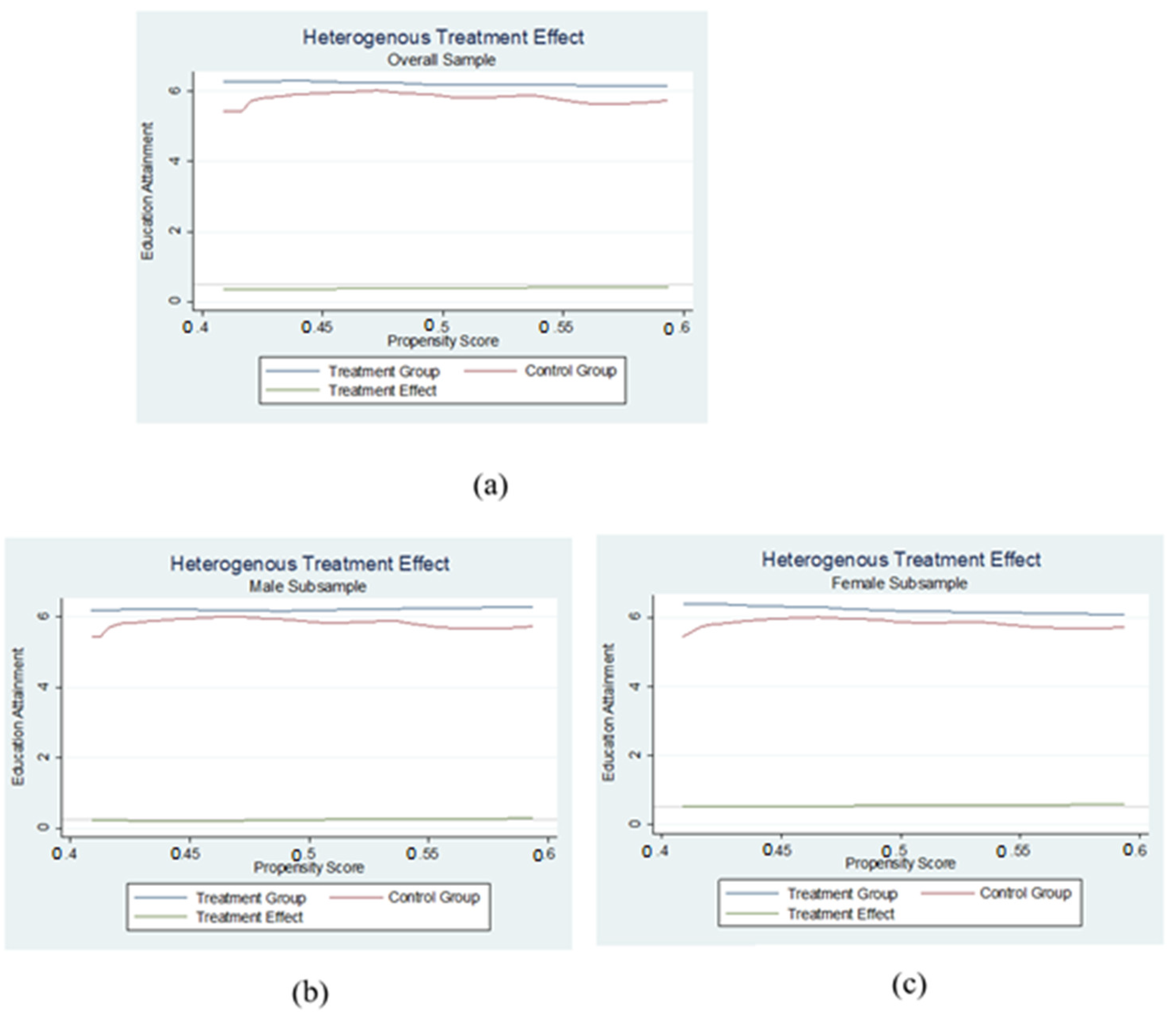
5.6. Non-Parametric Treatment Effect

Following the method of Paudel and Araujo, to consolidate the results obtained in Section 5.4, a kernel local polynomial regression of the average educational attainment on the probability of being treated via the implementation of the OCP was plotted, respectively, for both the treatment group and control group [33]. The results are shown in Figure 1. At each sub-figure, educational attainment for both the treatment group and the control group at each propensity score value was plotted together in the common support area. The difference between the treatment group and the control group defines the non-parametric treatment effect. The figurative results provide strong visible evidence for the conclusions obtained in Table 9. Specifically, it can be concluded from the result of the non-parametric treatment effect that the implementation of the OCP has a positive effect on the overall sample, male subsample, and female subsample and that the OCP has a larger effect on the educational attainment of the female subsample than in the male subsample and thus it is helpful in terms of decreasing the gender differences in education [21].

From Figure 1a, it can be observed that, at each value of the propensity score, the educational attainment of the treatment group is always higher than that of the control group in the common support area. The non-parametric treatment effect was defined as the difference in educational attainment between the treatment group and the control group. For the overall sample, the non-parametric treatment effect based on the kernel local polynomial regression keeps close but always lower than 0.5 years (see Figure 1a). The results in Table 9 are supported by Figure 1a. Firstly, it can be observed that the educational attainment of the treatment group is always larger than that of the control group at each value of the propensity score in the common support area. Furthermore, while the non-parametric treatment effect of the male subsample waves around 0.25 years (see Figure 1b), the non-parametric treatment effect of the female subsample waves around 0.5 (see Figure 1c). This means that the OCP’s marginal effect on educational attainment is higher in the female subsample than in the male subsample. Therefore, the results in Figure 1 show strong support for the former conclusion that the implementation of the OCP alleviates the gender education difference.

So far, it can be concluded that the ATT of the implementation of the OCP on educational attainment for the overall sample and two gender subsamples was positive and higher in the female subsample than in the male subsample. The conclusions are reinforced by checking the sensitivity to the potential unobservable factors and plotting the non-parametric treatment effect based on kernel local polynomial regression.

However, all of the above analyses were restricted to the micro field, and no macroeconomic factors have been involved until now. To extend the conclusion with the macro aspect, the OCP will be associated with the Chinese GDP per capita in Section 6.

6. The Effect of the OCP on Income Level

One may argue that educational attainment cannot proxy human capital completely since the latter represents ability in terms of work; even those who have no education experience could possess some human capital. To solve this issue, we replace education attainment with personal income to proxy human capital. On the other hand, income per capita is normally used as an economic growth index from the view of development economics. The relationship between the OCP and Chinese economic growth is not a new topic. The OCP’s effect on improving Chinese GDP per capita is arguable. The current studies considered this question from two aspects. On the one hand, Wang and Yao show that the Chinese economy has passed the Lewis turning point after which a shortage in the labor force will lead to low-speed economic growth [34]. Therefore, the implementation of the OCP possibly deteriorated the growth of the Chinese economy. On the other hand, improvements in terms of human capital accumulation played a large role in the increase in Chinese GDP per capita. Therefore, it is also possible that the OCP helped to promote the growth of GDP per capita through the Q–Q mechanism proposed by Becker and colleagues [1,2,3]. The Quality–Quantity trade-off refers to the mechanism introduced to describe the relationship between the number of children of a household and their quality in terms of education level and health situation. The theory points to the fact that there may exist a trade-off between the quality and quantity of children, i.e., under the restriction of some economic conditions (finance and time, for example); the fewer children that a household has, the healthier or more educated each child will be.). Although the existence of a Q–Q trade-off is being scrutinized in some developed countries (Angrist, Lavy & Schlosser, 2010), the former analysis of this research supports the validity of a Q–Q trade-off in China (see Section 6) [5]. Specifically, based on the conclusions obtained in Section 6 and Section 7 that the OCP has a positive effect on improved human capital per capita for both of the overall and the gender, in this part, the OCP will be connected with the OCP per capita to test its effect on the macro aspects. There is nothing new about this econometric framework. To remain consistent with the former analysis, the propensity score matching method was continued while changing the outcome variable to personal income. In this case, based on the data of CHFS 2013, pre-tax income and after-tax income were chosen to be the outcome variables.

The descriptive statistics are shown in Section 3, from which the increase in income after the implementation can be observed. Similar to the process of analyzing the OCP’s effect on educational attainment, a one-to-one nearest-neighbor matching with replacement was conducted. Firstly, a Logit model, in which the dummy variable of the OCP was a dependent variable, was built. For the marginal effect of the pre-treatment variables on implementation status, the results of CSA testing and post-matching balance were the same as those in the case of the educational attainment case (to avoid repeating the content, in this part, the specific results of the Logit model, CSA test, and the post-matching test were omitted. The propensity score of the overall sample varies from 0.409 to 0. and varies from 0.385 to 0.593 for the male subsample and from 0.410 to 0.610 for the female subsample). In this part, what matters is the formal result of the PSM process. The rest of this part is organized as follows: first,

Table 11. The marginal effect of OCP on income per capita.

Panel A. Pre-Tax Income
	Overall		Male		Female
	Pre-Matching	Post Matching	Pre-Matching	Post Matching	Pre-Matching	Post Matching
NNM	1397.050 (1125.516)	1723.058 (1157.910)	377.266 (1826.556)	488.707 (1903.058)	2314.761 * (1241,418)	2914.655 ** (1245.638)
KM	1397.050 (1125.516)	1714.194 (1152.403)	377.266 (1826.556)	714.263 (1893.209)	2314.761 * (1241,418)	2631.699 ** (1238.963)
Matching	No	Yes	No	Yes	No	Yes
Observations	11,525	11,525	5945	5945	5580	5580
Panel B. After-tax income
	Overall		Male		Female
	Pre-matching	Post matching	Pre-matching	Pre-matching	Post matching	Pre-matching
NNM	1540, 335 (1088.092)	1862.929 * (1117.627)	634.751 (1751.079)	757.462 (1821.040)	2338.767 * (1223.141)	2931.299 ** (1227.647)
KM	1540, 335 (1088.092)	1848.584 * (1112.387)	634.751 (1751.079)	959.199 (1811.747)	2338.767 * (1223.141)	2643.662 ** (1221.045)
Matching	No	Yes	No	Yes	No	Yes
Observations	11,525	11,525	5945	5945	5580	5580

Notes: (a) Table 11 shows the effect of OCP on personal income. (b) The standard errors in parentheses are shown in parenthesis. (c) *** p < 0.01, ** p < 0.05, * p < 0.1.

show the results of the PSM process separately for the overall sample, male subsample, and female subsample; second, to further consolidate the results obtained in Section 6.1, a sensitivity analysis and a non-parametric treatment effect calculation will be conducted separately in Section 6.2 and Section 6.3. All of the results will be shown for the overall sample and gender subsamples.

6.1. Marginal Effect of OCP on Individual Income

The results shown in Table 11 are interesting. The first two columns provide the ATT of the OCP on pre-tax income per capita and post-tax income per capita of the overall sample. It is evident that the marginal effect (ATT) of the OCP on after-tax income is significant only under 10% significance when using both the NNM and KM matching method. In addition to that, all of the other marginal effects did not pass the significance test even under 10% significance for the overall sample. This means that the OCP did not lead to improvements in terms of income per capita, or the impact was very small at least. However, based on the former conclusion of this research that the OCP had a significant effect in terms of increasing human capital per capita, this finding may indicate that the increase in human capital per capita only affected Chinese economic growth in a minor way. This conclusion is consistent with the argument of some earlier papers [34,35].

One may doubt this conclusion due to two concerns: firstly, transfer income and social programs are not counted into the income index, and secondly, the possibility of selection bias may impact the result. For the first problem, considering the core of this part, which can be restated as the causal relationship between the OCP and the ability to earn, the transfer income is thus not suitable in this case, although it is an important constituent for GDP computation. For the second concern, a sensitivity analysis for income per capita is conducted to judge whether the ATT is underestimated, based on the method of Diprete and Gangl [32]. The sensitivity analyses of pre-tax income and after-tax income were conducted, respectively, and the results are demonstrated in

Table 12. The sensitivity analysis for the income per capita of the hidden bias.

	Overall Sample				Male Subsample				Female Subsample
	Upper and Lower Bounds		p-Value		Upper and Lower Bounds		p-Value		Upper and Lower Bounds		p-Value
$\mathbf{e}\mathbf{x}\mathbf{p} \left(\mathbf{\gamma }\right)$	t-hat+	t-hat−	sig+	sig−	t-hat+	t-hat−	sig+	sig−	t-hat+	t-hat−	sig+	sig−
Panel A. The sensitivity analysis for pre-tax income
1	26848.3 ***	26,848.3 ***	0	0	33,772.5 ***	33,772.5 ***	0	0	18,793.4 ***	18,793.4 ***	0	0
1.25	26742.5 ***	27,010.3 ***	0	0	32,929 ***	34,152.8 ***	0	0	16,706.9 ***	19,333.7 ***	0	0
1.5	26715.2 ***	27,138.8 ***	0	0	31,022.1 ***	35,863.7 ***	0	0	16,706.9 ***	16,555.7 ***	0	0
1.75	26622.1 ***	27,205.1 ***	0	0	28,169 ***	36,944 ***	0	0	15,910.1 ***	21,285 ***	0	0
2	26609.4 ***	27,743.3 ***	0	0	27,219.3 ***	37,753.9 ***	0	0	15,308.8 ***	21,741.4 ***	0	0
2.25	26609.4 ***	27,244.6 ***	0	0	26,197.2 ***	38,709.9 ***	0	0	14,833.2 ***	21,974.3 ***	0	0
2.5	26543.1 ***	27,310.9 ***	0	0	26,190.3 ***	38,716.8 ***	0	0	14,541.1 ***	21,974.3 ***	0	0
2.75	26543.1 ***	27,376.4 ***	0	0	26,077.8 ***	38,716.8 ***	0	0	13,928.9 ***	22,217 ***	0	0
3	26516.3 ***	27,376.4 ***	0	0	26,077.8 ***	38,716.8 ***	0	0	13,744.3 ***	23,221.2 ***	0	0
Panel B. The sensitivity analysis for after-tax income
1	26,530.6 ***	26,530.6 ***	0	0	33,727.7 ***	33,272.7 ***	0	0	18,608.4 ***	18,608.4 ***	0	0
1.25	26,428.8 ***	26,687.1 ***	0	0	32,743.2 ***	33,758.2 ***	0	0	16,671.4 ***	19,219.5 ***	0	0
1.5	26,402 ***	26,810.8 ***	0	0	30,954.1 ***	35,371.8 ***	0	0	16,588.8 ***	19,716.1 ***	0	0
1.75	26,311.9 ***	26,874.7 ***	0	0	28,128.3 ***	36,519.5 ***	0	0	15,796 ***	21,552 ***	0	0
2	26,300.2 ***	26,910.9 ***	0	0	27,177.6 ***	37,534.8 ***	0	0	15,237.1 ***	21,556.4 ***	0	0
2.25	26,300.2 ***	26,912.7 ***	0	0	26,162.6 ***	38,147 ***	0	0	14,761.6 ***	21,788.6 ***	0	0
2.5	26,236.3 ***	26,976.5 ***	0	0	26,111.8 ***	38,197.7 ***	0	0	14,516.2 ***	21,788.6 ***	0	0
2.75	26,236.3 ***	27,039.5 ***	0	0	26,019.1 ***	38,197.7 ***	0	0	13,723.5 ***	22,031.9 ***	0	0
3	26,210.1 ***	27,039.5 ***	0	0	26,029.1 ***	38,197.7 ***	0	0	13,655.5 ***	22,837.8 ***	0	0

Notes: (a) exp (γ) provides the odds of differential assignment due to unobserved factors; t-hat+/t-hat− is the test- statistic with the null hypothesis: overestimation/ underestimation of treatment effect; sig+/sig− provides the p-value, assuming overestimation/underestimation of treatment effect; (b) ***, **, * means individually that the ATT is not sensitivity to the hidden bias at significance levels of 1%, 5% and 10%.

. Similar to the procedure in Section 4.2, the odds ratio of being treated increased gradually with a 25% step interval. From Table 12, it is clear that no matter the income index (pre-tax income or after-tax-income) used as the outcome variable, both t-hat+ and t-hat− were significant even when $\exp \left(\gamma \right)=3$, which means that the marginal effect (i.e., ATT) of the OCP on the income per capita was not underestimated and the conclusion is stubborn with increasing $\mathrm{e}\mathrm{x}\mathrm{p} \left(\gamma \right)$. Therefore, it can be concluded that the implementation of the OCP did not result in a significant effect in terms of improving income per capita based on the observations from CHFS2013.

When the same econometric methods were used on the male subsample to measure the effect of the OCP on male income per capita, the conclusion was consistent with that of the overall sample, i.e., the implementation of the OCP did not have a substantial effect on improving male income. This result is evidenced in the third and fourth columns of Table 11, in which all the estimators for the ATT on the male subsample are not significant. However, a different situation appeared in the female subsample, and it can be observed in the last two columns of Table 11. Specifically, the marginal effects of the OCP on individual income measured using traditional linear regression and PSM methods were demonstrated, respectively, in the last two columns of Table 11. Before matching, the OCP was believed to have increased female pre-tax income per capita by CNY 2314.761 and after-tax income per capita by CNY 2338.767 at the 10% significance level. Moreover, the marginal effect in the female subsample was larger after the matching process. Based on the NNM, the OCP was shown to improve female average pre-tax income by CNY 2914.655 and improve female average after-tax income by CNY 2931.299 at the 5% significance level. The ATT calculated using KM is quite similar to that calculated using NNM. Combined with the finding that OCP does not have a significant effect on personal income in the male subsample, this conclusion suggests that the implementation of OCP is probably helpful in decreasing gender differences in terms of income. It can be partly explained by the research results of Yang and Qiu [36], which suggest that the education differential occupies a high position among the contributors to income inequality [36].

6.2. Sensitivity Analysis

To further consolidate the conclusions in Section 6.1, a sensitivity analysis was conducted for the overall sample, male subsample, and female subsample to measure the sensitivity of the ATT calculated in Table 11 to the potential hidden bias. The results of the sensitivity analyses are shown in Table 12. It can be observed that all of the t-hat+ and t-hat− are significant at the significance level of 1%, which means that the ATTs calculated in Table 11 are not sensitive to the hidden bias. Precisely, the results in Table 12 show strong evidence that the implementation of the OCP had almost no effect on Chinese economic growth in the overall sample and male subsample but had a positive effect on increasing both the pre-tax income and after-tax income in the female subsample. Therefore, the implementation of the OCP was helpful in decreasing the gender differences in terms of individual income, although it was not effective in terms of economic growth at the overall level.

6.3. Non-Parametric Treatment Effect

Like de Araujo, the non-parametric treatment effect of the OCP on the income per capita was tested by running a kernel local polynomial regression [33]. The result of the non-parametric treatment effect shows that the implementation of the OCP has almost no effect on the increase in income per capita for the male subsample but has a significant positive effect on the increase in income per capita for the female subsample and is thus beneficial in terms of decreasing gender income differences. Due to space limitations, the figures are not displayed here.

7. Conclusions

This research shed light on the effect of the OCP on improving human capital per capita based on a propensity score matching (PSM) method based on the data of CHFS2013. The analysis was conducted separately for the overall sample, male subsample, and the female subsample. The result shows that the implementation of the OCP indeed improved the average human capital for the overall sample and two gender subsamples. Furthermore, the effect of OCP on improving human capital per capita is larger in the female subsample than that in the male subsample, which means that the average education difference is decreased between the male and female samples. To further understand what this conclusion means in the macroeconomics aspects, the PSM was extended to analyze the marginal effect of the OCP on the GDP per capita, which is measured by considering pre and post-tax income. The result shows substantial evidence that the OCP is also helpful in reducing gender income differences by improving the average individual income of females significantly while almost not affecting the individual income for the male subsample.

In this research, both the nearest-neighbor matching method and kernel matching method were used to calculate the ATTs of the OCP, and they produced similar conclusions. To further consolidate the conclusions obtained via the matching methods, the non-parametric treatment effect of OCP on both human capital and GDP per capita was also conducted for the overall sample, male subsample, and the female subsample, based on kernel local polynomial regression. Compared with the results of the matching methods, the non-parametric calculation result has the same conclusion when measuring the marginal effect of the OCP on human capital. In other words, the non-parametric regression shows substantial evidence of the significant effect of the OCP on human capital for the overall sample, male subsample and female subsample and the gender difference in human capital. When measuring the marginal effect on GDP per capita, the results of kernel local polynomial regression were reasonably close to those of the matching method, although a small marginal effect was observed on the overall sample and male subsample. In summary, a reliable conclusion is that the OCP is beneficial in terms of improving human capital for the overall sample and gender subsamples, improving GDP per capita for the female subsample, and decreasing human capital and income gender differences.

However, the above conclusion also indicates the potential risk of the current Chinese population policy. Since 2015, China has abandoned the OCP and is encouraging couples to have two births. The change may have a positive impact on economic development in the long term by preparing a larger labor force for the future. However, it is considered that the improvement in terms of human capital per capita for the whole sample and the individual income for females will be impacted negatively by degrading the fertility restrictions. In addition, gender equality will also be deteriorated by enlarging the gender differences between education and income. Therefore, the research suggested that when encouraging people to have a second birth, the relevant education policy should be matched. For example, the government could establish more schools, including kindergartens, primary schools, and middle schools, to adapt to the increasing population. In addition to that, the financial incentive is also considerable for families who have more than one child, especially when one of them is female, to esnure the education of children will not be negatively affected and that the gender differences will not be enlarged.

Despite the above innovations, this author recognizes the failure to apply the adjustment ATT estimator put forward by Abadie to correct the potential conditional bias of the simple nearest-neighbor matching [29]. Secondly, the difference in OCP policy intensity from county to county suggested by McElroy and Yang also failed to be included in the model [37]. These two flaws are left for future study.

References

1. Becker, G.S. An economic analysis of fertility. In Demographic and Economic Change in Developed Countries; Becker, G.S., Ed.; Princeton University Press: Princeton, NJ, USA, 1960; pp. 209–240. [Google Scholar]
2. Becker, G.S.; Tomes, N. An equilibrium theory of the distribution of income and intergenerational mobility. J. Polit. Econ. 1979, 87, 1153–1189. [Google Scholar] [CrossRef]
3. Zhang, J.S. The evolution of China’s one-child policy and its effects on family outcomes. J. Econ. Perspect. 2017, 31, 141–161. [Google Scholar] [CrossRef] [Green Version]
4. Hatton, T.J.; Martin, R.M. Fertility decline and the heights of children in Britain, 1886-1938. Explor. Econ. Hist. 2010, 47, 505–520. [Google Scholar] [CrossRef] [Green Version]
5. Angrist, J.; Lavy, V.; Scholosser, A. Multiple experiments for the causal link between the quantity and quality of children. J. Labor Econ. 2010, 28, 773–824. [Google Scholar] [CrossRef]
6. Galor, O. From physical to human capital accumulation: Inequality and the process of development. Rev. Econ. Stud. 2004, 71, 1001–1027. [Google Scholar] [CrossRef]
7. De La Croix, D.; Doepke, M. Inequality and growth: Why differential fertility matters. Am. Econ. Rev. 2003, 93, 1091–1113. [Google Scholar] [CrossRef] [Green Version]
8. Strulik, H.; Prettner, K.; Prskawetz, A. The past and future of knowledge-based growth. J. Econ. Growth 2013, 18, 411–438. [Google Scholar] [CrossRef]
9. Zhang, C. The evolution of Chinese family planning. Mark. Demogr. Anal. 2000, 6, 47–54. [Google Scholar]
10. Qian, Y.M.; Chen, J.M. The revolution of Mao’s thought about population and the reasons: An empirical analysis based on Mao’s statement of Chinese population. Mao Zedong Thought Study 2017, 34, 6–15. [Google Scholar]
11. Mao, Z.D. The Selected Works of MaoZedong; People’s Publishing House: Beijing, China, 1991. [Google Scholar]
12. Yang, K. The Overview of the Chinese Population and Family Planning; People’s Publishing House: Beijing, China, 2001. [Google Scholar]
13. Chen, W. The discussion about the evolution of the Chinese population during the “Cultural Revolution”. J. Cent. South Univ. 2011, 17. [Google Scholar]
14. Li, B.J.; Zhang, H.L. Does population control lead to better child quality? Evidence from China’s one-child policy enforcement. J. Comp. Econ. 2017, 45, 246–260. [Google Scholar] [CrossRef]
15. Ma, L.; Fang, X.M.; Lei, Z.; Cai, X.C. Does only child’s gender affect the fertility desire of only-child parents to bear a second child? Study Chinese Gen. Soc. Sur. 2016, 6, 17–26. [Google Scholar]
16. Ahn, N. Effects of the one-child family policy on second and third births in Hebei, Shaanxi and Shanghai. J. Popul. Econ. 1994, 7, 63–78. [Google Scholar] [CrossRef]
17. Liao, P.J. The one-child policy: A macroeconomic analysis. J. Dev. Econ. 2013, 101, 49–63. [Google Scholar] [CrossRef]
18. Li, J.L. China’s one-child policy: How and how well has it worked? A case study of Hebei Province, 1979-88. Popul. Dev. Rev. 1995, 21, 563–585. [Google Scholar] [CrossRef]
19. Rosenzweig, M.R.; Zhang, J.S. Do population control policies induce more human capital investment? Twins, birthweight, and China’s ‘one child’ policy. Rev. Econ. Stud. 2009, 76, 1149–1174. [Google Scholar] [CrossRef] [Green Version]
20. Liu, H. The quality-quantity trade-off: Evidence from the relaxation of China’s one-child policy. J. Popul. Econ. 2014, 27, 565–603. [Google Scholar] [CrossRef]
21. Qin, X.Z.; Zhuang, C.C.; Yang, R.D. Does the one-child policy improve children’s human capital in urban China? A regression discontinuity design. J. Comp. Econ. 2017, 45, 287–303. [Google Scholar] [CrossRef]
22. Almond, D.; Li, H.; Zhang, S. Land Reform and Sex Selection in China; Working Paper 19153; NBER: Cambridge, MA, USA, 2017. [Google Scholar]
23. Austin, P.C. An introduction to propensity score methods for reducing the effects of confounding in observational studies. Multivar. Behav. Res. 2011, 46, 399–425. [Google Scholar] [CrossRef] [Green Version]
24. Caliendo, M.; Kopeinig, S. Some practical guidance for the implementation of propensity score matching. J. Econ. Surv. 2008, 22, 31–73. [Google Scholar] [CrossRef] [Green Version]
25. Li, H.B.; Zhang, J.S.; Zhu, Y. The quantity-Quality Trade-off of children In a developing country: Identification using Chinese twins. Demography 2008, 45, 223–243. [Google Scholar] [CrossRef] [PubMed] [Green Version]
26. Erola, J.; Jalonen, S.; Lehti, H. Parental education, class and income over early life course and children’s achievement. Res. Soc. Strat. Mobil. 2016, 44, 33–43. [Google Scholar] [CrossRef] [Green Version]
27. Aakvik, A. Bounding a matching estimator: The case of a Norwegian training program. Oxford B. Econ. Stat. 2001, 63, 115–144. [Google Scholar] [CrossRef]
28. Abadie, A.; Imbens, G.W. Large sample properties of matching estimators for average treatment effects. Econometrica 2006, 74, 235–267. [Google Scholar] [CrossRef]
29. Abadie, A. Bias-corrected matching estimators for average treatment effects. J. Bus. Econ. Stat. 2011, 29, 1–12. [Google Scholar] [CrossRef]
30. Rosenbaum, P.R.; Rubin, D.B. The central role of the propensity score in observational studies for causal effects. Biometrika 1983, 70, 41–55. [Google Scholar] [CrossRef]
31. Essama-Nssah, B. Propensity Score Matching and Policy Impact Analysis: A Demonstration in Eviews; World Bank: Washington, DC, USA, 2006. [Google Scholar]
32. Diprete, T.A.; Gangl, M. Assessing bias in the estimation of causal effects: Rosenbaum bounds on matching estimators and instrumental variables estimation with imperfect instruments. Sociol. Methodol. 2004, 34, 271–310. [Google Scholar] [CrossRef] [Green Version]
33. Paudel, J.; de Araujo, P. Demographic responses to a political transformation: Evidence of women’s empowerment from Nepal. J. Comp. Econ. 2017, 45, 325–344. [Google Scholar] [CrossRef]
34. Wang, Y.; Yao, Y.D. Sources of China’s economic growth 1952–1999: Incorporating human capital accumulation. China Econ. Rev. 2003, 14, 32–53. [Google Scholar] [CrossRef] [Green Version]
35. Bosworth, B. Accounting for growth: Comparing China and India. J. Econ. Perspect. 2008, 22, 45–67. [Google Scholar] [CrossRef] [Green Version]
36. Yang, J.; Qiu, M.Y. The impact of education on income inequality and intergenerational mobility. China Econ. Rev. 2016, 37, 110–125. [Google Scholar] [CrossRef]
37. McElroy, M.; Yang, D.T. Carrots and sticks: Fertility effects of China’s population policies. Am. Econ. Rev. 2000, 90, 389–392. [Google Scholar] [CrossRef] [PubMed] [Green Version]
Figure 1. Non-parametric treatment effect on educational attainment. The overall sample, male subsample and female subsample are shown in figure (ac), respectively.
Sustainability 15 12373 g001