Numerical and Experimental Study on Flow Field around Slab-Type High-Rise Residential Buildings

Abstract

High-rise residential buildings often adopt rectangular cross-sections with large depth-to-width ratios. Moreover, the cross-sections have many grooves and chamfers for better ventilation and lighting. However, related research is lacking. This study performed wind tunnel tests and large eddy simulations (LES) on two typical buildings to analyze the surface wind pressures and flow fields around the buildings. The base moment spectra, along with the wind pressure coefficients, demonstrate that numerical simulation is capable of accurately representing the magnitudes and variations in wind loads along the height of the building. Furthermore, numerical simulation effectively captures the dominant energy distribution characteristics of fluctuating wind loads in the frequency domain. The shear layer separations, vortex shedding and reattachment phenomenon were observed. It was found that in the middle and lower parts of the buildings, the shear layer separation changed dramatically. Buildings with depth-to-width ratios close to 2 are minimally affected by changes in wind direction. However, for buildings with larger depth-to-width ratios, especially when the short side faces the wind, the reattachment of the shear layer and the shedding of wake vortices become crucial factors in generating fluctuating cross-wind loads. This emphasizes the significant impact of wind direction and plan dimensions on flow characteristics and aerodynamic behavior. When the building contained corners and grooves, the low-wind-speed area induced by the shear layer separation shrank and the reattachment point shifted closer to the windward facade.

1. Introduction

Nowadays, high-rise residential buildings are extensively utilized in China due to their numerous advantages. To optimize ventilation and lighting effects, elongated slab forms are commonly adopted in the design of high-rise residential buildings. As the building height increases, especially when steel structures are employed as the load-bearing system, issues concerning cross-wind and wind-induced responses become more prominent. These issues require meticulous consideration and thorough analysis to guarantee both the structural integrity and occupant comfort of high-rise residential buildings. As a result, researchers and engineers are dedicating their efforts to devising innovative strategies and solutions aimed at mitigating the negative impacts of wind on tall buildings while simultaneously enhancing their overall sustainability.

Many scholars have studied the aerodynamic characteristics of high-rise buildings with various cross-section shapes. Davenport pioneeringly studied the wind-induced response of high-rise buildings with different aerodynamic shapes [1]. Kwok investigated the wind-induced response of a tall building and found that horizontal slots, slotted corners and chamfered corners can cause significant reductions in both the along-wind and cross-wind responses [2]. Dutton studied the aerodynamic characteristics of three models of high-rise buildings with openings and found that building openings can notably reduce the dynamic effects and cross-wind bending moments caused by vortex shedding [3]. Dong et al. studied the wind pressure of high-rise buildings and found that vortex shedding is the primary cause of fluctuating wind pressure on building sidewalls [4]. Zhuang et al. investigated the wind load characteristics of rectangular high-rise buildings with different corner radii. They found that the windward corners with rounded edges experienced higher mean wind pressures and peak wind pressures compared to those with square corners [5]. Lin et al. studied the overall wind load on the surface of buildings with rectangular cross-sections. They found that when the depth-to-width ratio of the rectangular cross-section reaches a critical value, the drag coefficients reach the peaks [6]. Shen et al. conducted wind tunnel tests for high-rise buildings and analyzed how the shape coefficients vary with wind direction angles and aspect ratios [7]. Ke et al. investigated the effects of vertical ribs on the façade of high-rise buildings on wind loads and wind-induced response. They found that vertical ribs with a relative width of 4% can reduce mean force coefficients in the along-wind direction and attenuate cross-wind vibration by disrupting vortex shedding. Moreover, the ribs in the corner regions of the façade play a dominant role in disrupting vortex shedding [8].

In civil engineering, numerical simulation plays a crucial role in predicting loads on structures and optimizing design solutions [9,10]. With the development of computer technology and computational wind engineering theory, computational fluid dynamics (CFD) has developed into a supplementary tool for traditional wind engineering research methods (wind tunnel experiments and field measurements) [11]. Due to the complex flow field of the atmospheric boundary layer, the Reynolds-averaged Navier-Stokes (RANS) method was more commonly used for the numerical simulation of high-rise buildings [12,13]. Nie et al. and Yang et al. adopted the standard Reynolds stress turbulence model based on RANS to perform a numerical simulation of the steady flow field around a standard high-rise building model suggested by CAARC (Commonwealth Advisory Aeronautical Research Council) [14]. With the rapid increase in computer performance, large eddy simulation (LES) has attracted more and more attention and has been used to solve various wind engineering problems. It is found that the large eddies of the flow are dependent on the geometry while the smaller eddies are more universal. Due to the complexity and difficulty in accurately predicting small-scale turbulence, LES directly simulates the large-scale structures and uses a subgrid-scale model to parameterize the small-scale structures. By employing the LES method, we can better capture the dynamic behavior of turbulent structures and the transfer of turbulent energy, thereby improving the accuracy of flow simulations [15]. Shirzadi et al. investigated the accuracy of CFD simulations using the RANS model and LES in predicting mean and turbulent wind characteristics around a high-rise building. They compared the CFD results against measurements from a wind tunnel experiment. The study found that RANS and LES achieved similar accuracy in predicting mean wind velocity. However, LES was able to predict gust wind velocity with significantly higher accuracy compared to RANS [16]. Nozu et al. analyzed the aerodynamic load of high-rise buildings based on LES and found LES can better reproduce the non-isotropic and non-stationary characteristics of actual wind flow fields [17]. Aly used the LES method to analyze wind flow around buildings and validated it through full-scale experiments. By studying the effects of inflow boundary proximity, more accurate peak pressures were obtained [18]. Zheng et al. used the LES method to simulate the aeroelastic response of a square high-rise building. The results show that the aeroelastic response is mainly caused by along-wind buffeting and cross-wind vortex-excited vibration [19]. Ke et al. and Yang et al. also simulated the surface wind pressure of super-high-rise square buildings and analyzed the surface wind pressure drag [20,21]. Lubcke et al. [22] demonstrated that the application of the LES method not only accurately predicts the location of boundary layer separation and reproduces complex flow fields but also provides superior simulation of vortex structures around buildings, thus enhancing our understanding of flow fields.

The above studies involve various cross-section forms, but most of them are adopted by commercial buildings. High-rise residential buildings often adopt rectangular cross-sections with large depth-to-width ratios. Moreover, the cross-section has many grooves and chamfers used for better ventilation and lighting effects. Wind loads can have significant implications for the structural integrity and safety of tall buildings [23,24,25]. To mitigate these hazards, engineers and architects must carefully consider the wind loads during the design and construction phases of slab-type high-rise residential buildings [26,27]. However, related research is still lacking. This paper conducts wind tunnel tests and numerical simulations on the wind load on slab-type high-rise residential buildings. Firstly, wind tunnel pressure tests for rigid models and high-frequency force balance base (HFFB) tests were carried out on two typical slab-type buildings to obtain the basic characteristics of wind pressure on the building surfaces. Then, LES considering the gust wind effects was performed on these two buildings. The simulation results were compared with the wind tunnel test. Flow field analyses were carried out to explore the mechanisms that generate complex cross-wind fluctuating wind loads.

2. Wind Tunnel Test

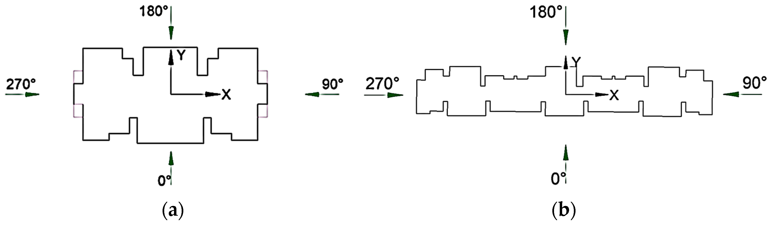
2.1. Building Configurations and Testing Model Configurations

The building group consists of 15 high-rise residential buildings, which are shown in Figure 1. Buildings no. 6 and no. 12 were selected as the main test objects with depth-to-width ratios (D/B) of 2 and 6, respectively. Building no. 6 has 34 floors above ground with a total height of 103 m, while Building no. 12 has a total height of 104 m. As shown in Figure 2a, Building no. 6 has a rectangular shape, with a longitudinal length of about 32.4 m and a transverse width of about 17.5 m. As shown in Figure 2b, Building no. 12 has a rectangular cross-section with a relatively large length and width, with a longitudinal length of about 86.8 m and a transverse width of about 15.7 m. Both the high-frequency force balance (HFFB) method and the synchronous multi-pressure sensing system (SMPSS) technique were adopted in wind tunnel tests to estimate the wind loads on these two buildings.

The experiments were carried out at the ZD-1 boundary layer wind tunnel at Zhejiang University, as shown in Figure 3. The wind tunnel has a testing section 4.0 m wide and 3.0 m high, and the maximum testing wind velocity is 50 m/s. The spire at the inlet of the wind tunnel and the rough elements at the bottom of the wind tunnel were used to simulate the wind speed profile. The model scale was 1:250, and no simplifications were made in the scale model. Thus, the dimensions of Building no. 6 are 116 × 61 × 389 mm, and the dimensions of Building no. 12 are 340 × 48 × 404 mm. The blockage ratio for the tested configurations was less than 6%, which meets the requirements for wind tunnel testing. No corrections for the blockage ratio were made.

Building no. 6 had 442 measuring points, and Building no. 12 had 494 measuring points. The pressure taps were connected to pressure scanners, which have 8 ports each. The pressure data were sampled at a frequency of 312.5 Hz, with a total sampling duration of 30 s, which could represent 10 min in full scale using a velocity scale of 1/5, leading to a time scale of 1/93.34. In total, time series of 10,000 pressure coefficients per tap were obtained for each wind direction and configuration. The tests included 24 different wind direction angles with a step size of 15 degrees, as defined in Figure 2.

The mean and fluctuating wind pressure on the measuring points can be directly measured using SMPSS. Then, by integrating the pressure over the control area, the wind pressure on the measuring point layer can be determined. On the other hand, the mean and fluctuating base forces can be measured directly through the HFFB tests. Subsequently, by taking into account the dynamic properties of the building, the corresponding dynamic responses such as base bending moments can be determined.

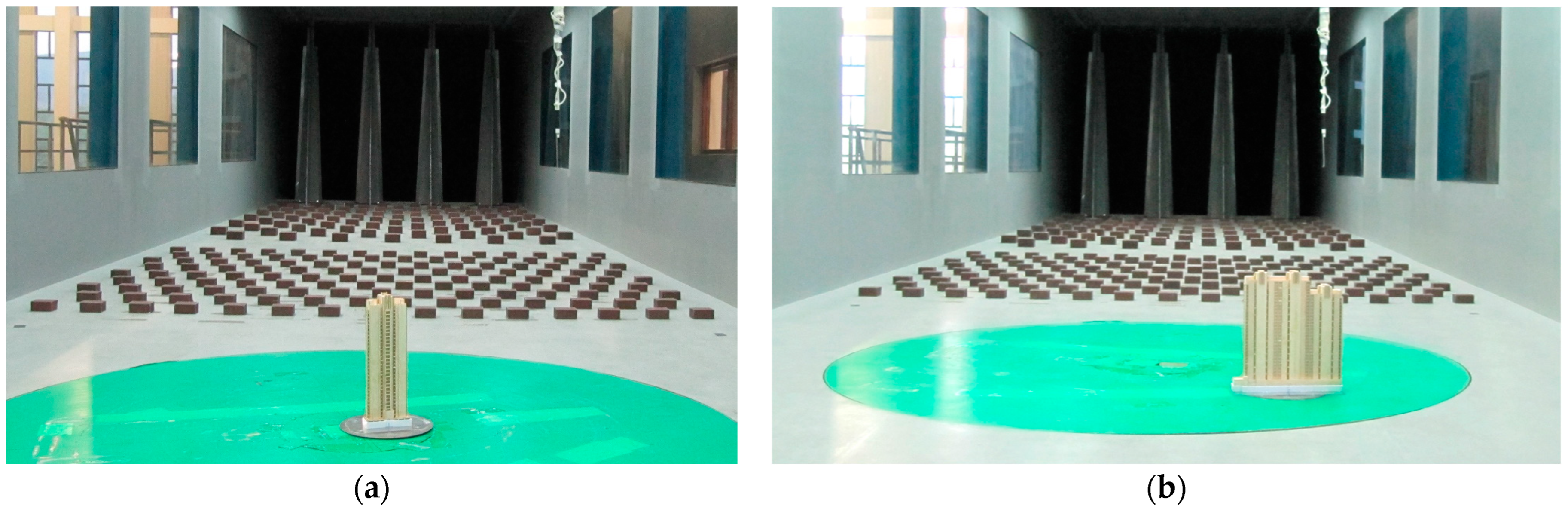
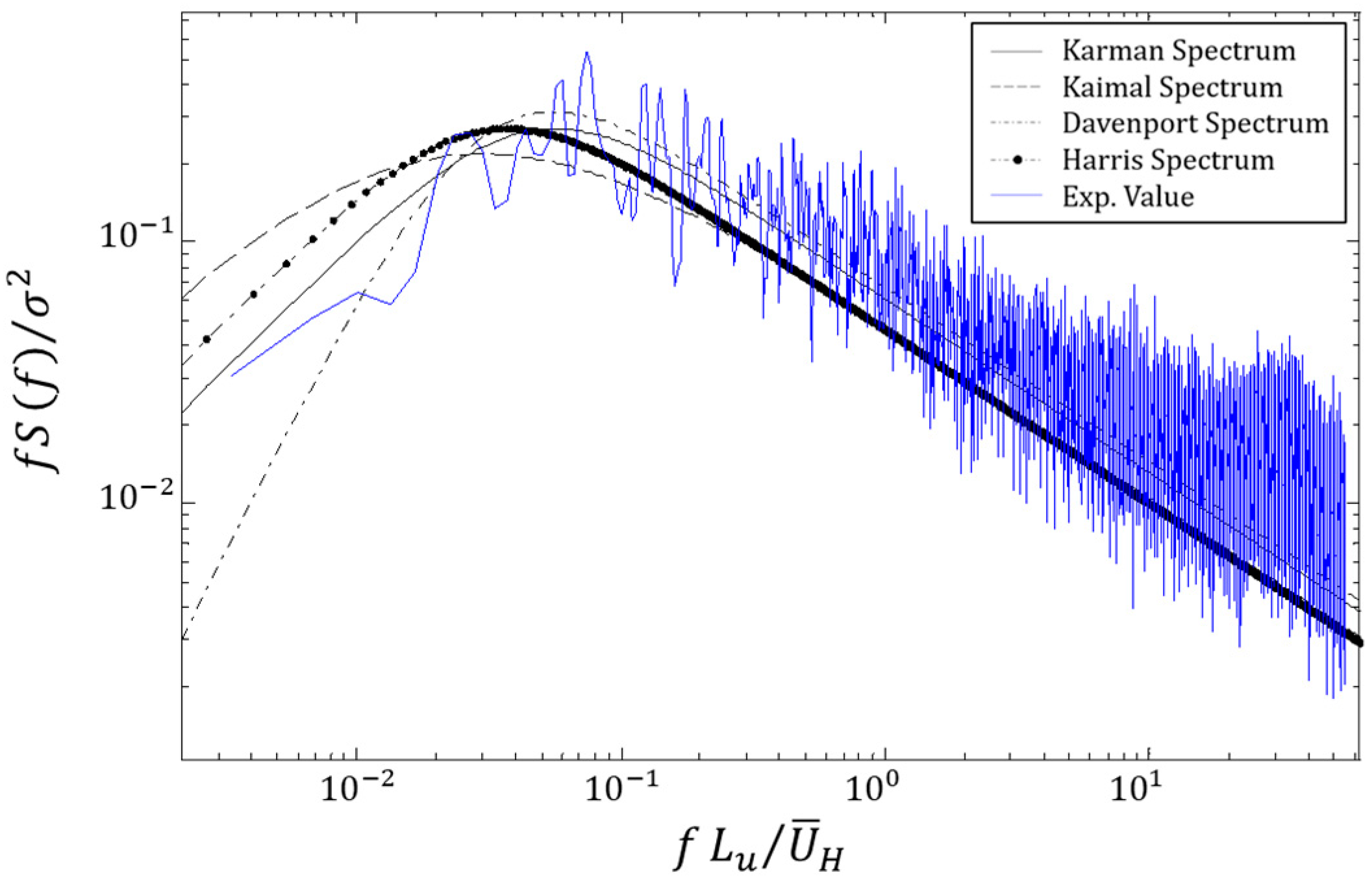
2.2. Wind Tunnel and Wind Field Simulation

The measurements were made with a reference wind speed of 10.7 m/s at a height of 0.6 m above the wind tunnel floor, in a region where the wind speed is uniform. This corresponds to a height of 150 m on the actual building. At this height, the design wind speed for a 100-year return period is 28.3 m/s for the actual building. Tests and calibrations were performed before the wind tunnel tests. The terrain in which the building group is located was classified as category B, with the ground roughness exponent of 0.16. It is worth noting that this study is based on real engineering projects with terrain categories predetermined according to the Chinese load code [28]. We acknowledge the importance of surface roughness length in atmospheric studies and its influence on airflow patterns. Many researchers have focused on this topic and obtained valuable results. In this paper, we specifically analyze the impact of the D/B ratio. The basic wind pressure is 0.45 kN/m² for a 50-year return period. The mean wind speed varies exponentially with height and can be expressed as Equation (1) [28].

$$\frac{{\bar{U}}_z}{{\bar{U}}_{10}}=(\frac{z}{10}{)}^{\alpha }$$

(1)

where ${\bar{U}}_z$ is the mean wind speed at height $z$, ${\bar{U}}_{10}$ is the mean wind speed at a height of 10 m, and $\alpha$ is the ground roughness exponent.

The turbulence intensity along the height can be expressed as Equation (2) according to the Japanese specification [29]. In this test, the turbulence intensity I = 16.75% is required at a height of 30 m.

$$I\left(z\right)=0.1(\frac{z}{H_T}{)}^{-\alpha -0.5}$$

(2)

where $I\left(z\right)$ is the turbulence intensity at height z and $H_T$ is the gradient wind height.

The measured wind profiles and target wind profiles are compared in Figure 4, where ${\bar{U}}_H$ represents the mean wind velocity at the building roof height, H. In Figure 4, “Exp. Value 1”, “Exp. Value 2” and “Exp. Value 3” refer to the three sets of experimental values obtained during the wind field measurements. An excellent match is achieved, indicating that the simulated wind field meets the requirements of the target values.

Figure 5 displays the comparison between the measured streamwise velocity spectrum and various empirical spectra at an equivalent full-scale height of z = 125 m. The parameters used in the graph include $f$ for frequency, $S\left(f\right)$ for power spectral density, $L_u$ for integral length scale, and ${\sigma }^2$ for the variance in turbulent wind. The simulated wind speed spectrum shows good agreement with the Von Karman spectrum.

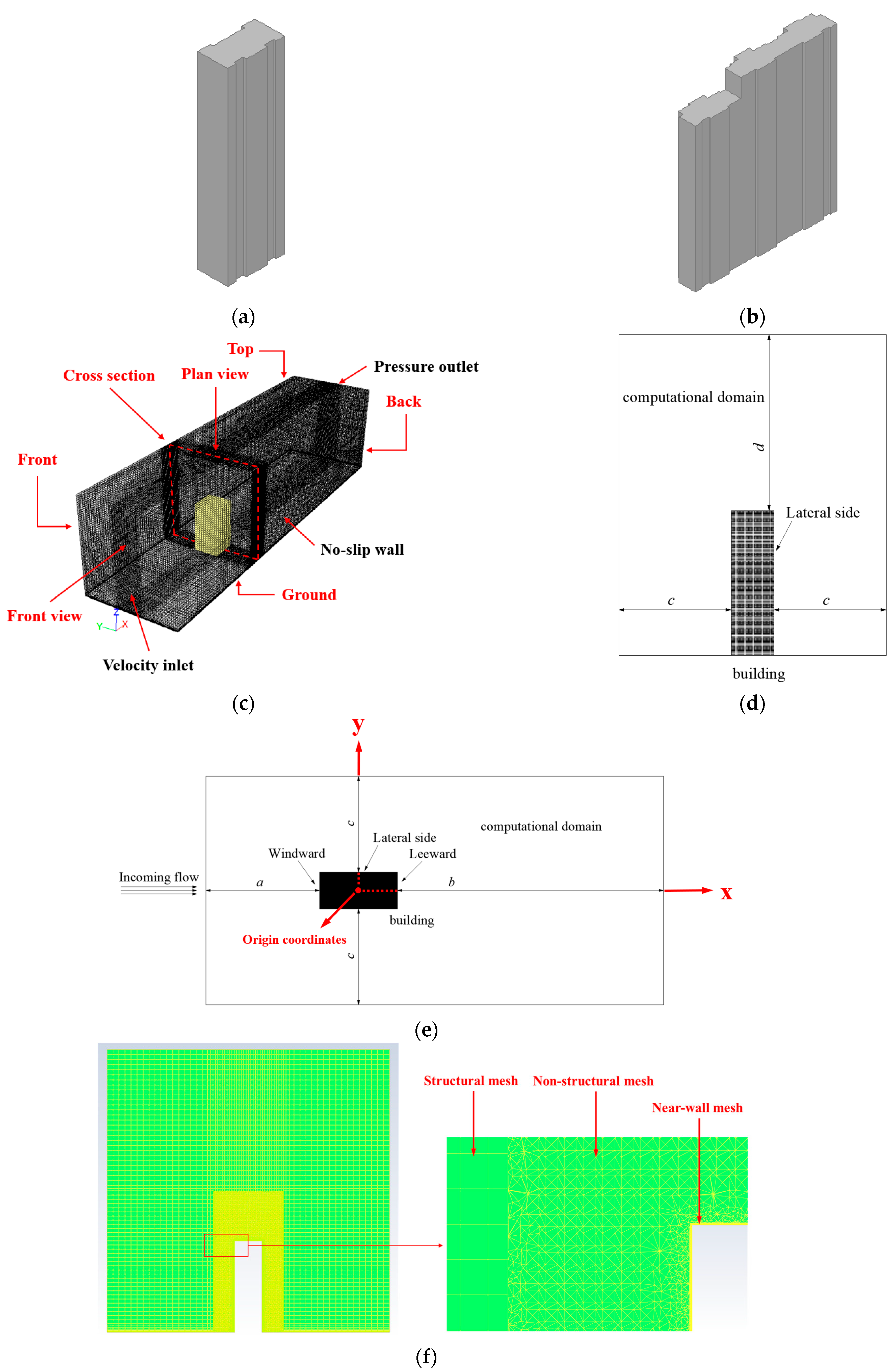
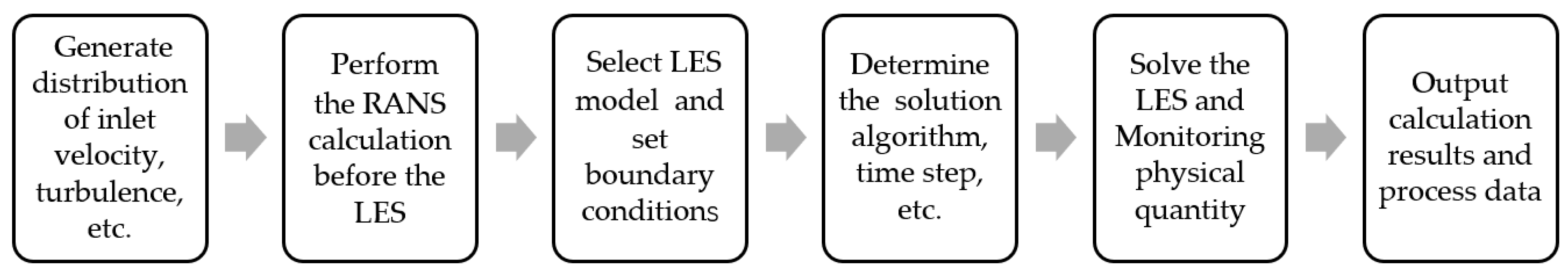
3. Numerical Simulation

Due to the high requirements of mesh size in LES, the same scale ratio of 1:250 was adopted in numerical simulation in order to control the total number of meshes and compare it with wind tunnel tests. The dimensions of Building no. 6 are 116 × 61 × 389 mm, and the dimensions of Building no. 12 are 340 × 48 × 404 mm. This dimension represents the main cross-sectional structure of the solid profile, with the largest dimension aligned along the principal axis. It also serves as the size of the comparative models. According to the length scale ratio, wind speed scale ratio and similarity criterion, the scale ratios of the variables involved in numerical simulation can be determined, which are shown in

Table 1. Scale factor in CFD.

Variable Name	Scale Factor
Length	1:250
Wind speed	1:1
Time	1:250
Wind pressure	1:1

.

Unsteady flow calculations were carried out for Building no. 6 and Building no. 12. For Building no. 6 and no. 12, wind direction angles of 0° and 90° were selected to analyze the influence of incoming wind direction. In order to analyze the influence of the building facade on the flow field, two smooth rectangular cross-sectional buildings were set up as a comparison. The numerical simulation conditions involved in this paper are shown in

Table 2. Numerical simulation conditions.

Case	Description	Corresponding Wind Tunnel Test	Selected Wind Direction
Case A	Real building facade	Building no. 6 (single building)	0°, 90°
Case B	Smooth rectangular facade
Case C	Real building facade	Building no. 12 (single building)
Case D	Smooth rectangular facade

.

The mesh division of the calculation domain was carried out using the software ICEM (17.0), since the groove size is too small and it is easy to generate over-deformed meshes during mesh division if the building facade is accurately modeled. Therefore, the building facade is appropriately simplified. The simplified model is shown in Figure 6a,b. Meanwhile, considering the requirements of convergence, the growth rate of adjacent mesh sizes cannot be too large. In order to control the total number of meshes and improve computational efficiency, the calculation domain is divided into a core area and a peripheral part. The core area adopts the non-structural mesh division method, and the peripheral part adopts the structural mesh division method. The computational domain configuration for the numerical simulations is illustrated in Figure 6. The yellow-highlighted area in Figure 6c represents the core area, which adopts the non-structural mesh division method, while the remaining parts correspond to the peripheral area, which adopts the structural mesh division method.

The dimensions of the computational domain are listed in

Table 3. Computational domain size (mm).

Case	Region	Length
Case A, Case B	a	2000
	b	4000
	c	1000
	d	800
Case C, Case D	a	2000
	b	4000
	c	1500
	d	800

. The lengths chosen in Table 2 for Case A and Case B (4000 mm, 2000 mm, 1000 mm and 800 mm) and for Case C and Case D (4000 mm, 2000 mm, 1500 mm and 800 mm) are based on the sizes of the objects being considered. Larger objects require larger lengths to accommodate their size, while smaller objects can be adequately represented with smaller lengths. The requirements aim to obtain a computational domain that meets the requirement of blockage effects and adequate inflow length and outflow distance for accurate simulation of the flow features around the building using LES.

To accurately simulate the flow behavior, certain boundary conditions are imposed. As shown in Figure 6c, the velocity inlet was set up on the front surface. To compare with wind tunnel experiments, the average wind speed and turbulence intensity along the height are modeled to vary exponentially, following Equations (1) and (2). Considering that the FLUENT software (17.0) only provides built-in boundary definitions with constant wind speed along the height, a user-defined function (UDF) is employed to achieve the desired exponential wind profile. This approach ensured accurate simulation of the wind conditions. The boundary conditions of the top, bottom, and side surfaces were specified as the no-slip wall. The pressure outlet was applied on the back surface. These carefully selected boundary conditions enable the simulation to capture realistic airflow dynamics within the wind tunnel testing section.

According to the boundary layer theory, the turbulent zone near the wall can be divided into three layers: laminar sublayer, buffer region and turbulent region. The laminar sublayer is dominated by viscous forces, the turbulent region is dominated by turbulent effects, and the buffer region is influenced by both. This is mainly affected by the roughness near the wall surface. Therefore, the exponential wind speed profile is actually valid in the area above a certain height from the wall surface [30]. In order to accurately calculate velocity gradients within the boundary layer, the inflation grid technique is utilized specifically for the lowest layer adjacent to both the ground and building surfaces.

In FLUENT, the influence of roughness near the wall surface is mainly described by non-dimensional wall distances y+. The near-wall mesh is usually encrypted since the thickness is usually required to be much smaller than the size of the computational domain meshes. In this study, 10 layers of boundary layer mesh were set near the wall surface, with a minimum mesh size of 0.05 mm, as shown in Figure 6f. As a result, the total number of mesh is 4,807,920 for Building no. 6 and 4,312,295 for Building no. 12.

In this study, to ensure steady-state convergence, the y+ values on the majority of ground and building surfaces are maintained below 10. However, in specific regions on the windward surface of the building, the y+ values are relatively large, approximately 30. Nonetheless, these values still comply with the computational requirements needed for accurate simulations.

Figure 7 gives a flow chart of the numerical simulation process. Prior to the LES calculation, the RANS method was used for steady-state calculation to generate the initial flow field and accelerate the convergence of the unsteady calculation. For the steady-state calculation, the SST-k-ω model was selected as the turbulence model, which can better simulate the separated flow near the building facade. An enhanced wall function was used as the wall function. The SIMPLE algorithm was adopted to decouple pressure and velocity, and a second-order upwind scheme was utilized to spatially discretize the equations in the simulations. For the LES calculation, the Smagorinsky-Lilly subgrid-scale (SGS) model was used. The bounded central-differencing scheme was used to discretize the convection term in the filtered momentum equation. Time discretization was second-order implicit, and the time step was set to 0.001 s. Using a small time step can effectively capture essential information from numerical simulation and facilitate the attainment of a converged solution. The calculations were performed on a workstation with eight thread. On average, it took approximately 20 h to process one simulation case. A total of 2500 time steps were calculated, which is equivalent to an actual time of 10.42 min (assuming the time scale between numerical simulation and real wind field is 1:250), satisfying the calculation requirements.

4. Results and Discussion

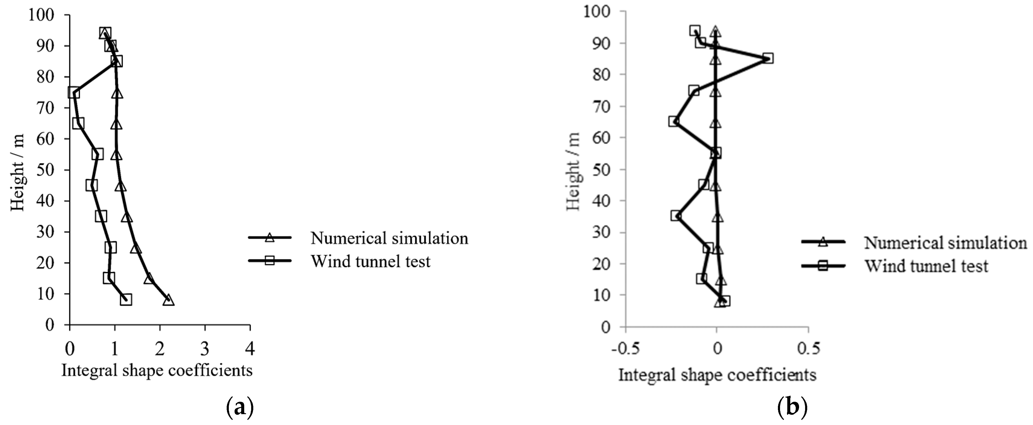
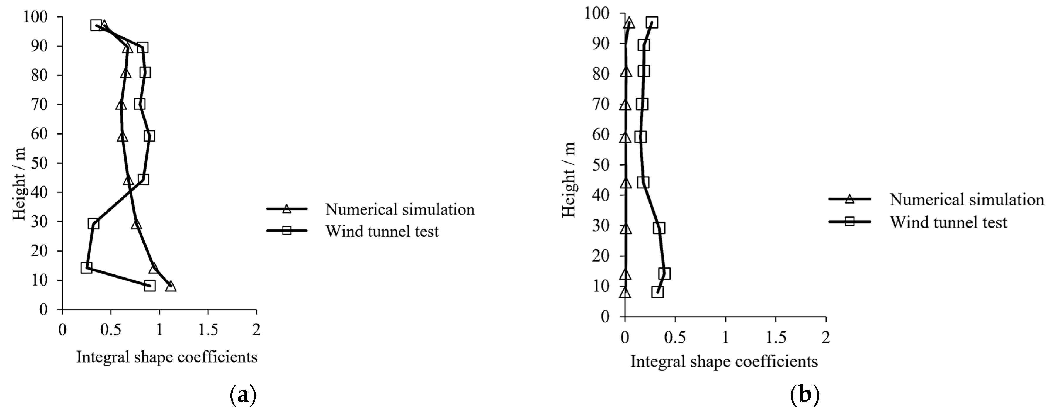
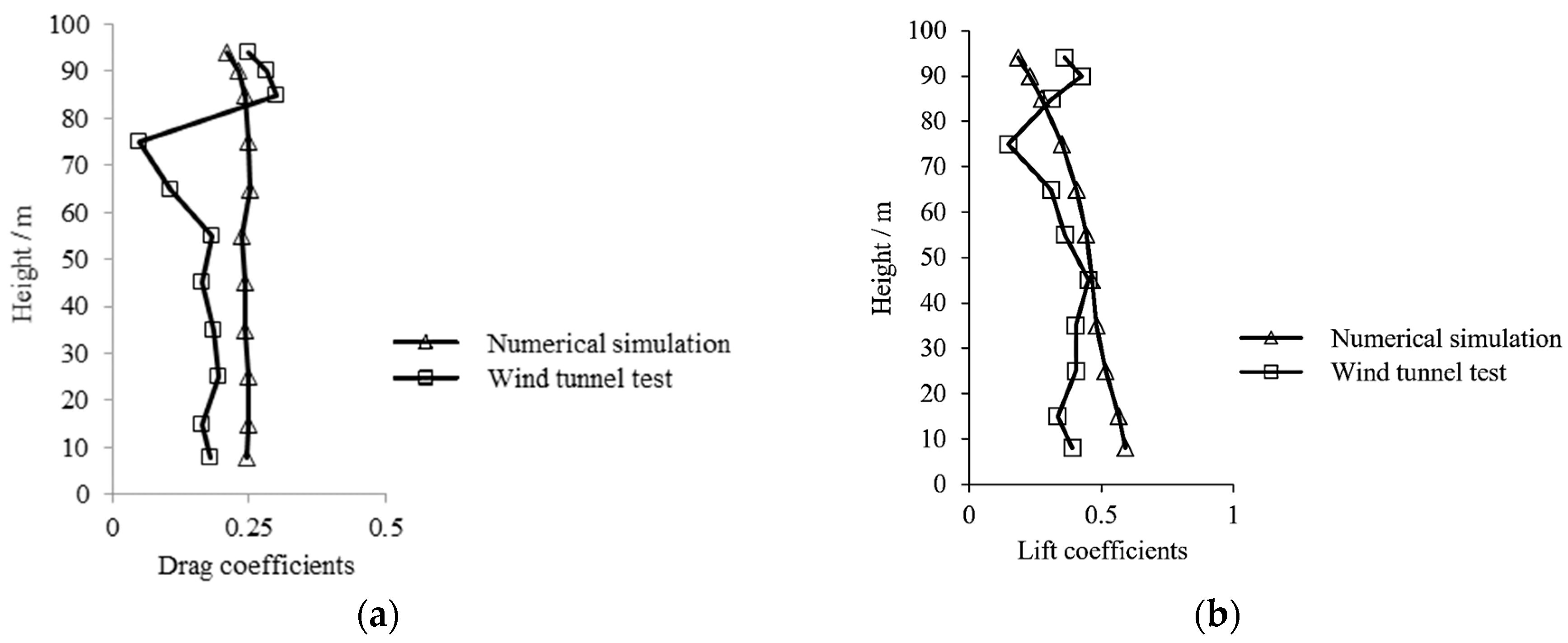
4.1. Comparison of Experimental and Numerical Results

The integral shape coefficients of floors can reflect the magnitude of the static wind load of the structural floor, defined as

$${\mu }_s=\frac{F}{{\mu }_z{w}_{0}L}$$

(3)

where $F$ is the wind load per unit height; ${\mu }_z$ is the height variation coefficient of wind pressure; $w_0$ is the basic wind pressure; and $L$ is the projection width of the floor.

Figure 8 and Figure 9 depict a comparison of the integral shape coefficients between the numerical simulation and wind tunnel testing results. For Building no. 6, as illustrated in Figure 8, the integral shape coefficients in the along-wind direction obtained from the numerical simulation were slightly higher, whereas the variation tendency was comparable between the numerical simulation and wind tunnel testing. However, for the integral shape coefficients in the cross-wind direction obtained from the numerical simulation, the variation trend along the height is less significant, and the range of values is narrower compared with the wind tunnel test results. For Building no. 12, as illustrated in Figure 9, the integral shape coefficients in the cross-wind direction obtained from the numerical simulation were similar to Building no. 6, while the integral shape coefficients in the along-wind direction presented divergent results. For the region above half of the building height, the along-wind integral shape coefficients from the numerical simulation were lower than those obtained from the wind tunnel testing. In contrast, the situation was opposite below half of the building height.

The fluctuating wind pressure, also termed the root mean square (RMS) wind pressure, can be decomposed into along-wind and cross-wind components, which are denoted as ${\sigma }_D\left(z\right)$ and ${\sigma }_L\left(z\right)$, respectively. For convenience of comparison, normalized RMS wind pressure coefficients were employed, which are defined as:

$$C_D^{\prime }(z)=\frac{{\sigma }_D\left(z\right)}{A{q}_{ref}}$$

(4)

$$C_L^{\prime }(z)=\frac{{\sigma }_L\left(z\right)}{A{q}_{ref}}$$

(5)

where $A$ is the frontal area per unit height at location z and $q_{ref}$ is the reference wind pressure.

Figure 10 and Figure 11 show the comparison of fluctuating wind pressure between numerical simulation and the wind tunnel test. Specifically, for Building no. 6 (Figure 10), the results from numerical simulation are greater than the results from the wind tunnel test. For Building no. 12 (Figure 11), the results from numerical simulation are less than the wind tunnel test data. Despite the relatively large uncertainties associated with fluctuating wind pressures due to their small magnitudes, numerical simulations are capable of capturing the general trend of fluctuating wind pressure variations with height.

In general, both wind tunnel tests and numerical simulations can capture the wind loading characteristics around buildings. However, there is a smoother variation along the height in the values obtained from numerical simulations compared to the results of wind tunnel tests. This discrepancy can be attributed to simplifications made in the numerical simulation model, particularly the omission of grooves and chamfers present in the physical wind tunnel model. These features in the wind tunnel model can influence the flow behavior and turbulence near the building surfaces, resulting in variations in pressure distributions and force coefficients.

The base moment power spectra can reflect the aerodynamic characteristics caused by fluctuating wind pressures. The base moment power spectra $S_x$ can be calculated by using Equation (6):

$$S_x(\omega )=\underset{T_0\to \infty }{lim}\frac{1}{2\pi T_0}{\left|X\left(i\omega \right)\right|}^2$$

(6)

where $T_0$ is the duration time of the time-series data; $X\left(i\omega \right)$ is the frequency domain data, which are obtained by converting the time-series data to the frequency domain through Fourier transform. The time-series base moment data are obtained directly from high-frequency dynamic balance tests.

The base moments are defined with respect to the axes of the building (for the axes definition, refer to Figure 2: the base moment spectra about the x-axis ($S_{Mx}$), the base moment spectra about the y-axis ($S_{My}$) and the torsional moment spectra about the z-axis ($S_{Mz}$). Figure 12 and Figure 13 show a comparison of the base moment power spectra about the y-axis. As depicted in Figure 12, for Building no. 6, the power spectrum of base moment $S_{My}$ under numerical simulation conditions peaks at 0.16 Hz for numerical simulation. Likewise, the power spectrum of the base moment also peaks at 0.15 Hz in the wind tunnel test. However, the maximum energy of the numerical simulation at 0 Hz is substantially lower than that of the wind tunnel test data. This discrepancy may be due to the simplification of the CFD model. For Building no. 12 as given in Figure 13, both the base moment spectra obtained from numerical simulation and wind tunnel test exhibit a primary frequency peak at an identical frequency (0.03 Hz). However, the numerical simulation results demonstrate more concentrated energy relative to the wind tunnel test outcomes. The power spectra of the base moments $S_{My}$ and $S_{Mz}$ exhibit similar trends. It is implied that the numerical simulations capture the energy distribution characteristics of the fluctuating wind loads in the frequency domain with superior accuracy.

These results, together with the wind pressure coefficients, demonstrate that the numerical simulations can represent the magnitudes of wind loads and their variations along the height of the building. Additionally, they can effectively capture the dominant energy distribution characteristics of fluctuating wind loads in the frequency domain.

However, it is worth noting that in order to achieve computational convergence, certain simplifications are made in the numerical simulation process. Additionally, the placement of measurement points is constrained by the grid, which makes it challenging to accurately capture wall pressure on the real building surface. Therefore, it is crucial to acknowledge the existence of unrealistic parameters in the numerical simulations, as they can contribute to certain discrepancies.

4.2. Three-Dimensional Vortex Characteristics Analysis

Time histories of the flow field around Buildings no. 6 and no. 12 are analyzed to gain insights into the flow characteristics at different heights. Through the LES, the horizontal wind velocity vector diagrams and the vertical wind velocity vector diagrams around the buildings could be obtained. The flow fields at the 2500th time step, corresponding to a prototype time of 10.42 min, are examined.

4.2.1. Effects of Wind Directions

Figure 14 shows the horizontal wind velocity vector diagrams of Building no. 6 at the height of 0.5 H, showcasing the vortex structure characteristics at different wind directions. The flow lines in the figure indicate the direction of the wind, while the color scheme represents the velocity in the XY plane, measured in meters per second (m/s). It can be seen that under both wind directions (0° and 90°), there are obvious shear layer separation phenomena on both sides of the windward face. The shear layer develops downstream along the length of the building, eventually separating from the edges and generating alternating vortices in its wake. These vortices induce fluctuating pressures on the side walls of the building that vary periodically over time. The width of the low-wind-speed region within the shear layer is closely related to the projections of the windward face of the building. Notably, it is observed that this width tends to be smaller when the wind direction is perpendicular (90°) to the building as compared to when it aligns with the building (0°). Moreover, altering the wind direction does not result in significant variations in flow characteristics.

Figure 15 presents the horizontal wind velocity vector diagrams of Building no. 12 at a height of 0.5 H, showcasing the flow characteristics under different wind directions. When the wind is perpendicular to the long edge of the building, as depicted in Figure 15a, the flow patterns resemble those observed in Building no. 6. This includes shear layer separation along both sides of the windward face, downstream progression and subsequent detachment leading to vortex shedding in the wake region. However, when the wind acts perpendicular to the short edge of the building, as shown in Figure 15b, distinct variations in flow characteristics are observed. In this case, following the shear layer separation, an alternating reattachment phenomenon occurs on both sidewalls. In addition to this reattachment phenomenon, the wake region also experiences a certain amount of vortex shedding.

To summarize, for buildings with depth-to-width ratios close to 2, changes in wind direction do not significantly affect the flow characteristics. However, for buildings with larger depth-to-width ratios, especially when the longer side faces the wind, the reattachment of the shear layer and the shedding of wake vortices play a crucial role in generating fluctuating cross-wind loads. This highlights the influence of the building’s plan dimensions and wind directions on the flow characteristics and aerodynamic behavior. Buildings with larger depth-to-width ratios and specific orientations can experience different flow patterns and increased fluctuating loads due to the reattachment of shear layers and vortex shedding.

4.2.2. Effects of Building Heights

Figure 16 provides a comparison of the horizontal wind velocity vector diagrams at different heights of Building no. 6. When combined with Figure 14a, it becomes apparent that the flow characteristics vary significantly with height. At the bottom and mid-height of the building, the alternating shear layer separations on both sides are highly asymmetric. This means that the separation points on each side of the building do not occur simultaneously. As a result, the vortex-shedding region downstream of the building becomes irregular and varies in width. This irregularity results in fluctuating cross-wind loads. In contrast, at the top of the building, the shear layer separations on both sides are more stable. This means that the separation points occur at a similar location and exhibit less asymmetry. Consequently, the low-wind-speed region within the wake remains within a relatively narrow range. The stability of the shear layer separation at the top of the building can be attributed to one significant factor: the reduced interference at greater heights. As the building rises higher, it experiences less interference from the ground and surrounding structures. This reduced interference allows for a more consistent flow pattern and a more stable shear layer separation. Also, it is assumed that from a certain height, the influence on the creation of eddies will be given mainly by the upper part of the building. The variation in horizontal wind velocity vector diagrams at different heights of Building no. 12 exhibits similar patterns, as shown in Figure 17. On the windward side, there is a noticeable phenomenon of shear layer separation where the wind velocity undergoes a rapid change. It is worth noting that, as shown in Figure 17b, at a height of 0.9 H, Building no. 12 transitions from three units to two units, resulting in a change in its structural shape. However, the separation of the shear layer remains similar to the original cross-section before the reduction in units. In regions without the presence of the building, the wind speeds are relatively lower, while the area of rapid wind velocity change remains the same as at a height of 0.5 H, corresponding to the maximum dimension of the structure’s cross-section.

As the height of Building no. 6 and Building no. 12 is very similar, their vertical wind velocity vector diagrams exhibit a high degree of similarity. Therefore, only the vertical wind velocity vector diagrams of Building no. 6 are given as an example, as shown in Figure 18. The non-homogeneous wind speed observed in the figures can be attributed to the presence of turbulence in the incoming flow. The complexity of turbulence leads to non-uniformity in the incoming flow velocity. It can be observed that the vortex shedding is primarily concentrated at the bottom and mid-height of the building. The vortex shedding generated at the top of the building diminishes rapidly within a relatively small range due to the disturbance from the airflow above the roof. The irregular vortex shedding distributed behind the building weakens gradually with increasing distance from the leeward side of the building and eventually restores to the wind speed distribution of the incoming atmospheric boundary layer. The region significantly affected by the building wake is approximately 4 H.

Overall, the reduced interference at greater heights plays a crucial role in stabilizing the shear layer separation at the top of the building. This stability contributes to a narrower and more controlled wake region with a relatively low wind speed compared to the irregular vortex shedding observed at lower heights.

4.2.3. Effects of Surface Roughness of Building

Figure 19 illustrates the horizontal wind velocity vector diagrams of smooth rectangular buildings at a height of 0.5 H, where H represents the height of the building. By comparing these diagrams with Figure 14b and Figure 15b, it is found that these surface roughness variations do not significantly alter the overall flow patterns around the buildings. This means that the fundamental flow behavior remains largely unaffected by surface roughness. However, the presence of chamfers and grooves, which are design features, noticeably modifies the extent of shear layer separation. Buildings with chamfers and grooves exhibit a smaller low-wind-speed region compared to smooth rectangular buildings. This reduction in the size of the low-wind-speed region can be attributed to the depletion of energy within the circulating and impinging flows inside the grooves. The presence of these features disrupts the flow and creates additional turbulence. Additionally, the inclusion of chamfers and grooves shifts the reattachment point closer to the windward facade of the building. This shift in the reattachment point can have implications for the distribution of pressure and loads on the building facade.

Overall, the surface roughness of the building has minimal influence on the overall flow behavior, but the presence of design features like chamfers and grooves can significantly modify the flow characteristics. These features can reduce the size of low-wind-speed regions and alter the position of the reattachment point, thereby affecting the aerodynamic performance and loads on the building.

In summary, the overall flow field around the building is closely related to wind directions, building height, and depth-to-width ratio. The size of the low-wind-speed area and the location of the reattachment point are affected by the surface roughness. Shear layer separation and wake vortex shedding are the dominant mechanisms affecting the wind load on buildings.

5. Conclusions and Recommendations

This study provides insights into the complex flow field around high-rise residential buildings. These buildings commonly have rectangular sections with large depth-to-width ratios and grooves. Specifically, it focuses on investigating the characteristics of crosswind vortex shedding and reattachment, as well as the influence of wind directions and geometric dimensions of buildings on the characteristics of turbulent wind. The main conclusions are as follows:

(1)

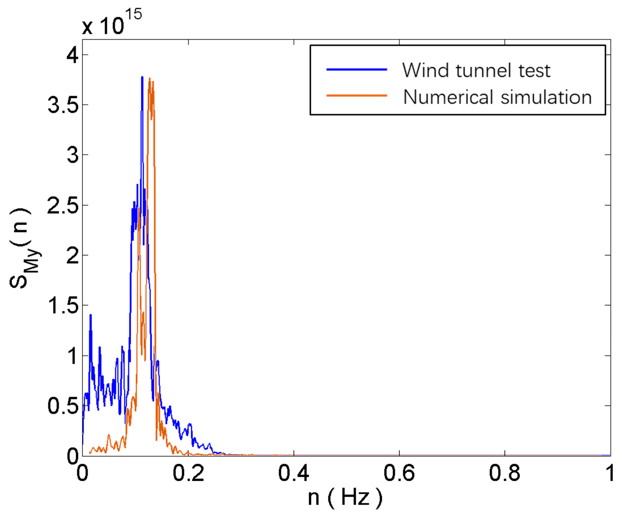
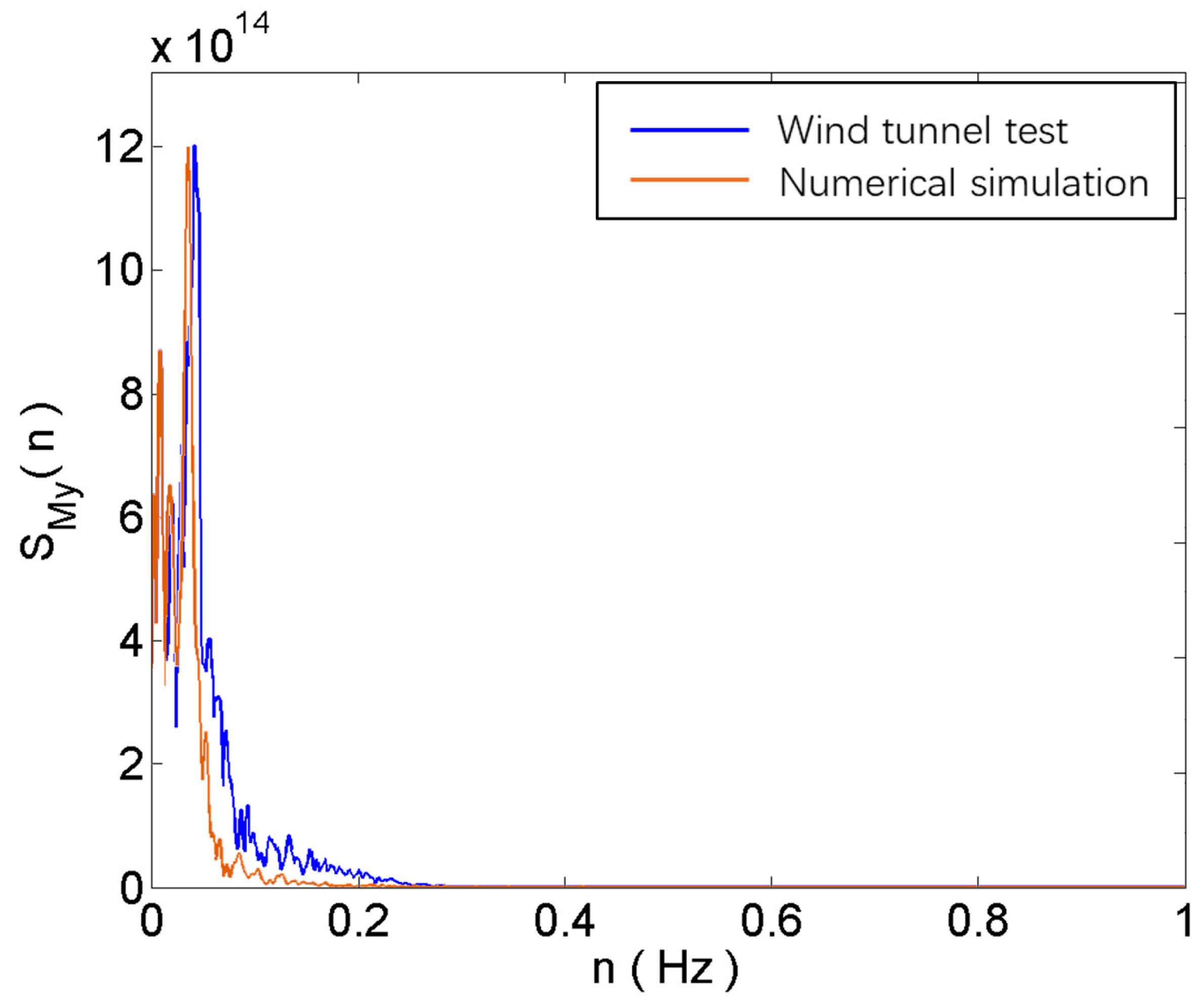
A comparative analysis between computational results and wind tunnel test data under similar conditions demonstrates that LES calculations effectively capture the magnitudes of and variations in wind loads along the height. Additionally, LES can better reflect the spectral characteristics of wind loads caused by vortex shedding. However, it is worth noting that numerical simulations involve simplifications. As a result, numerical wind tunnel results cannot completely replace wind tunnel experiments.

(2)

For buildings with a D/B ratio of 2, the fluctuating wind pressure in the along-wind direction is lower than that in the crosswind direction. Despite this difference, their trends along the height are similar, with the extreme values and inflection points occurring at the same positions. At higher D/B ratios (approximately 6), the fluctuating wind pressure coefficient in the along-wind direction does not change significantly and remains concentrated in the range of 0.1–0.2. However, the fluctuating wind pressure coefficient in the crosswind direction increases significantly, with the maximum value changing from 0.45 to 0.7.

(3)

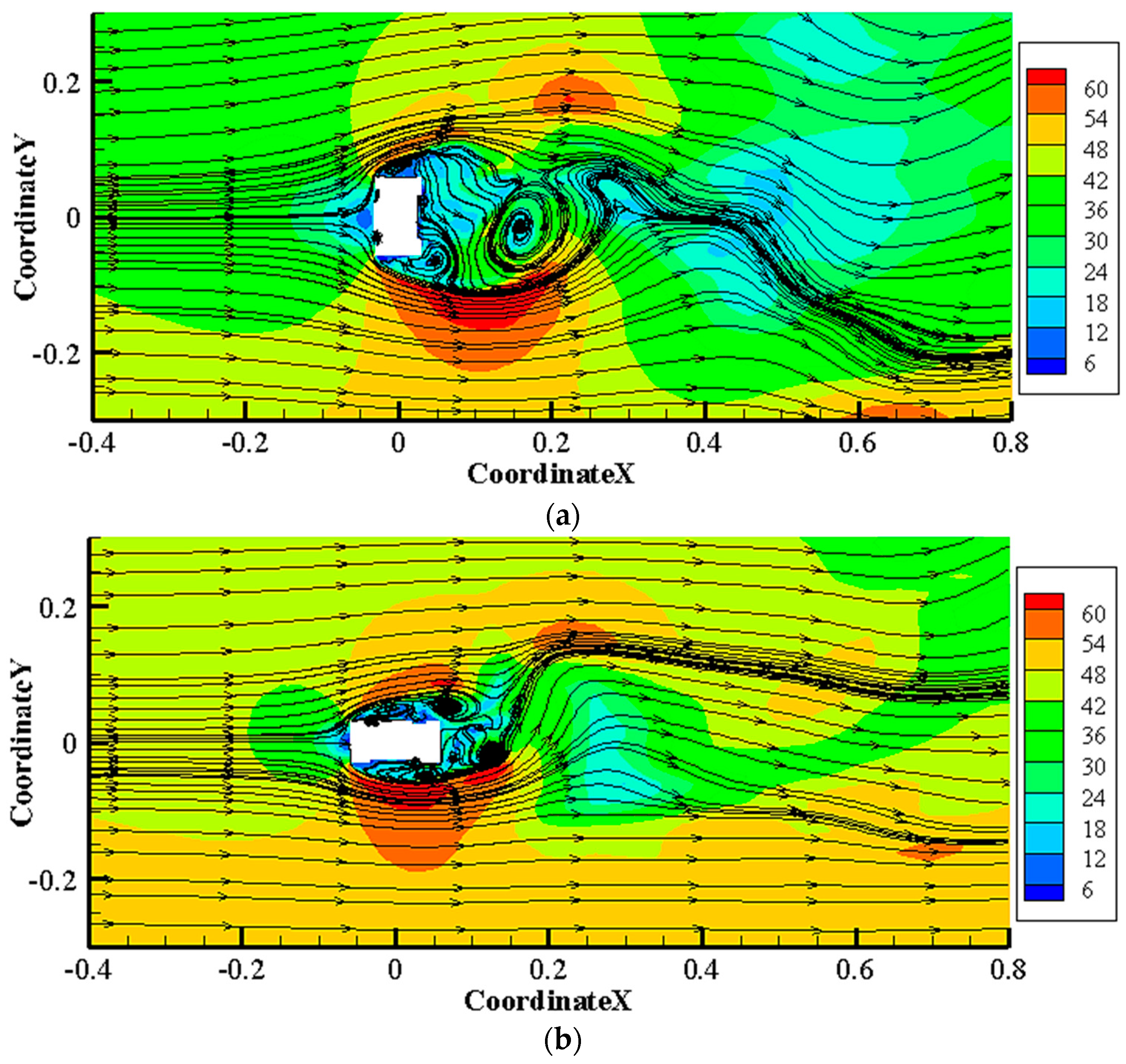
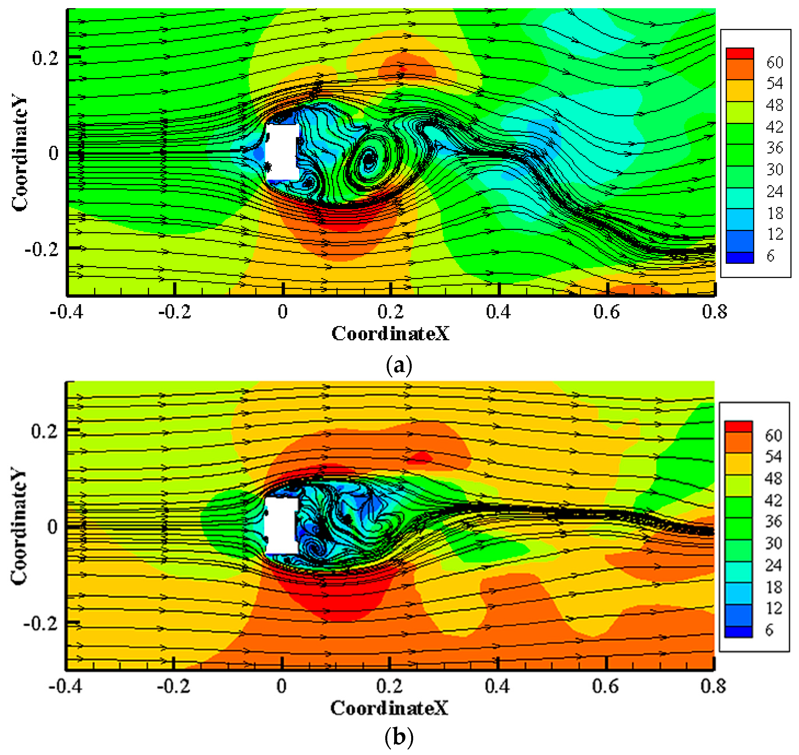
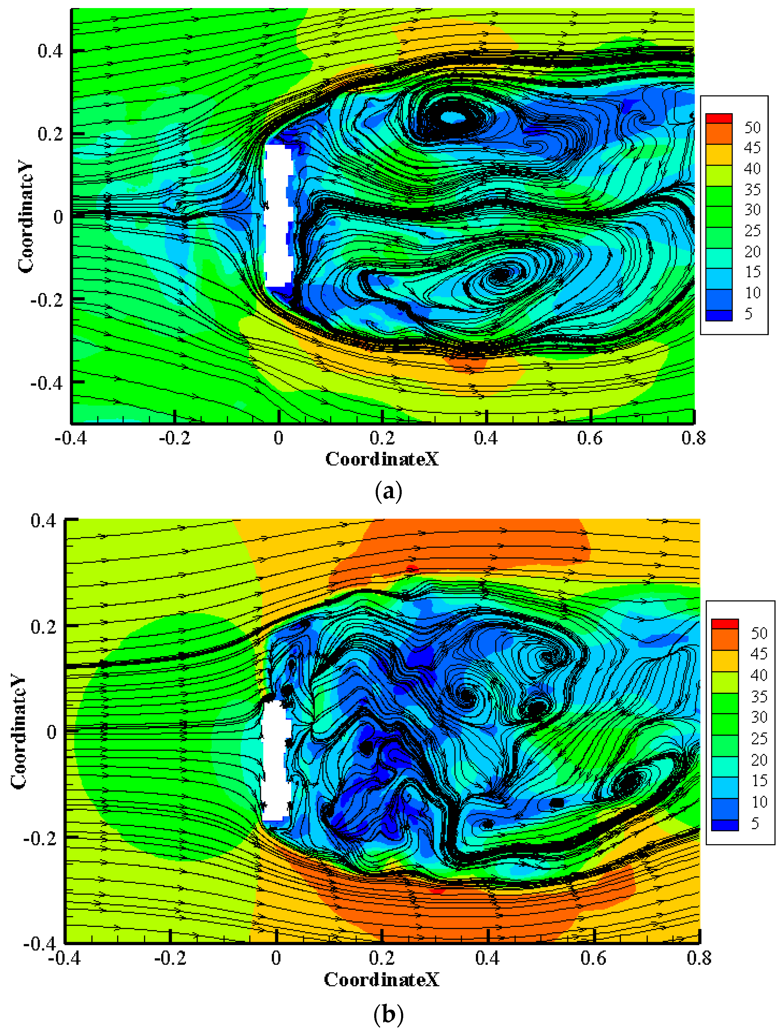
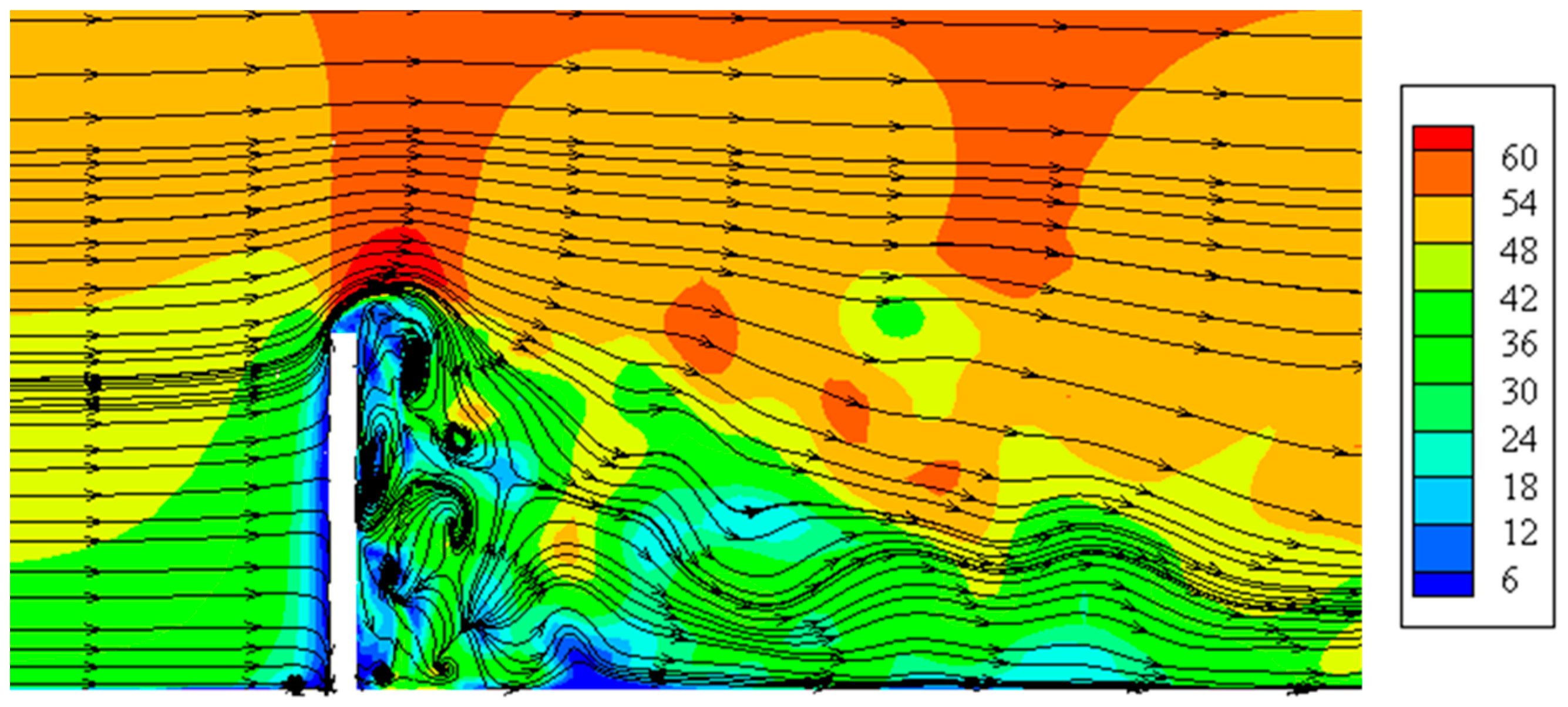
Shear layer separation appears on both lateral sides of the building. The separated shear layers develop downstream and eventually lead to the formation of staggered vortex shedding in the wake. Vertically, vortex shedding primarily occurs at the bottom and mid-height of the building. The vortex shedding generated at the roof is disturbed by the air flowing over the top of the building and diminishes rapidly within a relatively small range. It is assumed that from a certain height, the influence on the creation of eddies will be given mainly by the upper part of the building.

(4)

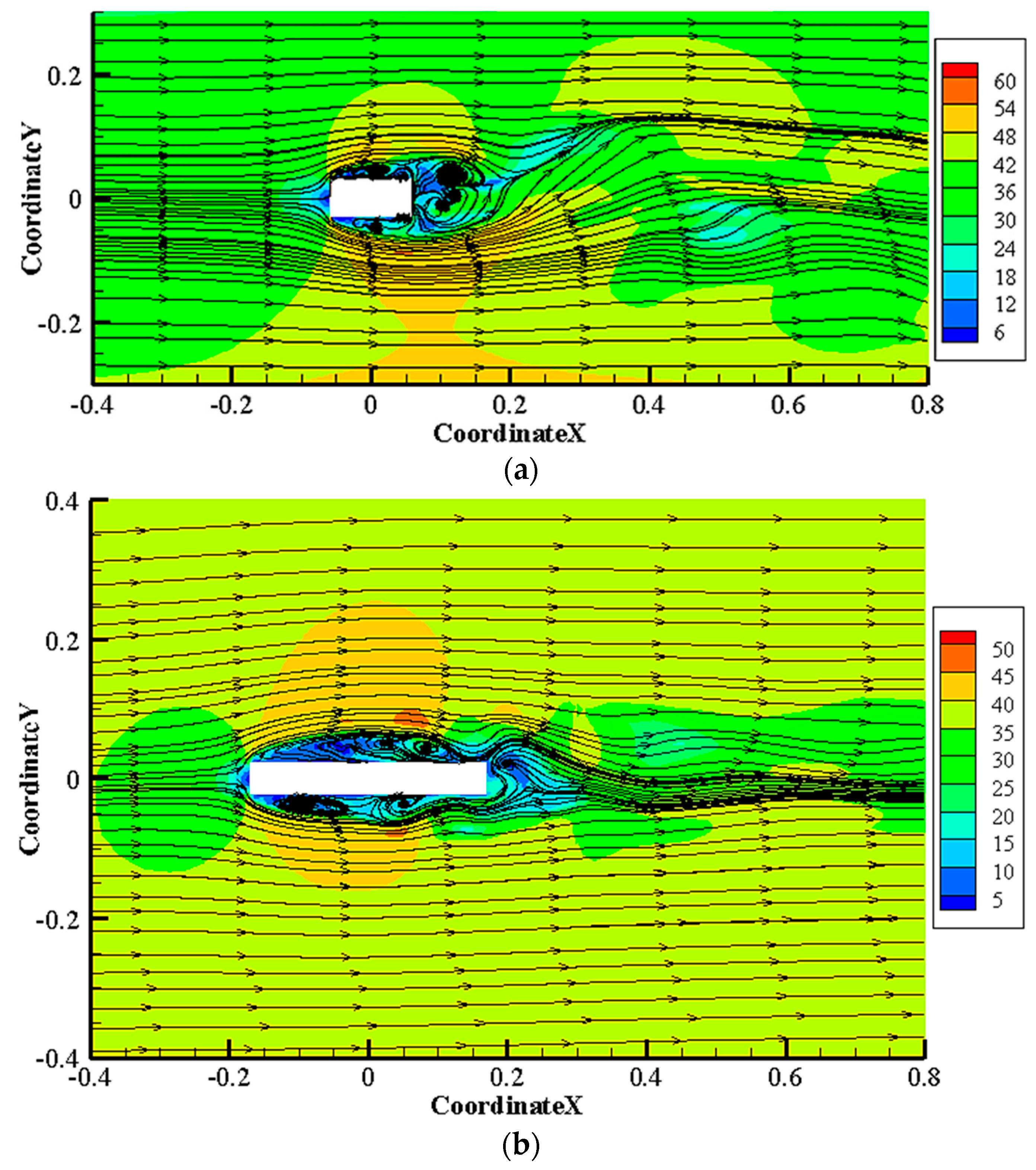
The overall flow field around the building is closely related to height and D/B ratio. The shear layer separations at the bottom and mid-heights of the building are highly asymmetric, causing irregular vortex shedding. At the top of the building, the shear layer separations are more stable, with the wake width relatively consistent. At lower aspect ratios (depth-to-width ratios close to 2), shear layer separation can cause fluctuations in crosswind loads. At higher aspect ratios (depth-to-width ratios close to 6), shear layer reattachment and wake vortex shedding lead to fluctuations in crosswind loads.

(5)

The size of the low-wind-speed area and the location of the reattachment point is affected by the surface roughness. When the building has corners and grooves, the separated flow region becomes smaller and the position of the reattachment point is closer to the windward surface. Adding textures to a building’s surface, such as grooves and stripes, can change the way fluids interact with the surface, thereby reducing the force of the wind.

For further research, it is recommended to conduct experimental and numerical studies specifically on slab-type high-rise buildings. The focus should be on wind resistance design, considering the influence of wind load on the building and implementing appropriate measures to enhance the building’s wind resistance. The measures may include, but are not limited to, strengthening the structural strength of the building, increasing lateral support, and considering the impact of wind on different components such as facades, roofs, and openings. Furthermore, studying the aerodynamics of slab-type buildings can help optimize their design and improve their overall performance in terms of wind resistance.

References

1. Davenport, A.G. The response of six building shapes to turbulent wind. Philos. Trans. R. Soc. Lond. Ser. A Math. Phys. Sci. 1971, 269, 385–394. [Google Scholar] [CrossRef]
2. Kwok, K.C.S. Effect of building shape on wind-induced response of tall building. J. Wind Eng. Ind. Aerodyn. 1988, 28, 381–390. [Google Scholar] [CrossRef]
3. Dutton, R.; Isyumov, N. Reduction of tall building motion by aerodynamic treatments. J. Wind Eng. Ind. Aerodyn. 1990, 36, 739–747. [Google Scholar] [CrossRef]
4. Dong, X.; Zhao, X.; Ding, J.; Zhuang, X. Wind pressure characteristics on a high-rise building with rectangular section. J. Build. Struct. 2016, 37, 116–124. [Google Scholar]
5. Zhuang, X.; Zheng, Y.; Zheng, X.; Dong, X. Wind load characteristics of rectangular high-rise buildings with various rounded corner ratios. J. Build. Struct. 2018, 39, 1–8. [Google Scholar]
6. Lin, N.; Letchford, C.; Tamura, Y.; Liang, B.; Nakamura, O. Characteristics of wind forces acting on tall buildings. J. Wind Eng. Ind. Aerodyn. 2005, 93, 217–242. [Google Scholar] [CrossRef]
7. Shen, G.; Qian, T.; Luo, J.; Yu, S.; Lou, W. Study of wind loading on rectangular-sectioned high-rise buildings with various length-to-width ratios. J. Hunan Univ. Nat. Sci. 2015, 42, 77–83. [Google Scholar]
8. Ke, Y.; Shen, G.; Yang, X.; Xie, J. Effects of Surface-Attached Vertical Ribs on Wind Loads and Wind-Induced Responses of High-Rise Buildings. Sustainability 2022, 14, 11394. [Google Scholar] [CrossRef]
9. Song, Y.; Chen, X.J.; Zou, B.P.; Mu, J.D.; Hu, R.S.; Cheng, S.Q.; Zhao, S.L. Monitoring Study of Long-Term Land Subsidence during Subway Operation in High-Density Urban Areas Based on DInSAR-GPS-GIS Technology and Numerical Simulation. Comput. Model. Eng. Sci. 2023, 134, 1021–1039. [Google Scholar] [CrossRef]
10. Bao, Y.J.; Huang, Y.; Liu, G.R.; Wang, G.Y. SPH simulation of high-volume rapid landslides triggered by earthquakes based on a unified constitutive model. Part I: Initiation process and slope failure. Int. J. Comput. Methods 2020, 17, 1850150. [Google Scholar] [CrossRef]
11. Huang, S.; Li, Q.S.; Xu, S. Numerical evaluation of wind effects on a tall steel building by CFD. J. Constr. Steel Res. 2007, 63, 612–627. [Google Scholar] [CrossRef]
12. Zheng, X.; Montazeri, H.; Blocken, B. CFD simulations of wind flow and mean surface pressure for buildings with balconies: Comparison of RANS and LES. Build. Environ. 2020, 173, 106747. [Google Scholar] [CrossRef]
13. Agrawal, S.; Wong, J.K.; Song, J.; Mercan, O.; Kushner, P.J. Assessment of the aerodynamic performance of unconventional building shapes using 3D steady RANS with SST k-ω turbulence model. J. Wind Eng. Ind. Aerodyn. 2022, 225, 104988. [Google Scholar] [CrossRef]
14. Nie, S.; Zhou, X.; Zhou, T.; Shi, Y. Numerical simulation of 3D atmospheric flow around a bluff body of CAARC standard high-rise building model. J. Civ. Archit. Environ. Eng. 2009, 31, 40–46. [Google Scholar]
15. Yang, L.; Huang, M.; Lou, W. Hybrid simulation of three dimensional fluctuating wind fields around tall buildings. J. Zhejiang Univ. Eng. Sci. 2013, 5, 824–830. [Google Scholar]
16. Shirzadi, M.; Tominaga, Y. CFD evaluation of mean and turbulent wind characteristics around a high-rise building affected by its surroundings. Build. Environ. 2022, 225, 109637. [Google Scholar] [CrossRef]
17. Nozu, T.; Tamura, T.; Okuda, Y.; Sanada, S. LES of the flow and building wall pressures in the center of Tokyo. J. Wind Eng. Ind. Aerodyn. 2008, 96, 1762–1773. [Google Scholar] [CrossRef]
18. Aly, A.M.; Gol-Zaroudi, H. Peak pressures on low rise buildings: CFD with LES versus full scale and wind tunnel measurements. Wind Struct. 2020, 30, 99. [Google Scholar] [CrossRef]
19. Zheng, D.; Gu, M.; Zhang, A. LES based numerical simulation of aeroelastic response of a 3D tall building. J. Build. Struct. 2013, 34, 97. [Google Scholar]
20. Ke, S.; Wang, H. Large Eddy Simulation Investigation of Wind Loads and Interference Effects on Ultra High-rise Connecting Buildings. J. Hunan Univ. Nat. Sci. 2017, 44, 53–62. [Google Scholar]
21. Yang, Y.; Wan, T.; Wang, K.; Xie, Z. Numerical Simulation Research on Combined Wind and Stack Effects of a Super High-rise Building. J. Hunan Univ. Nat. Sci. 2018, 45, 10–19. [Google Scholar]
22. Lubcke, H.; Schmidt, S. Comparison of LES and RANS in bluff-body flows. J. Wind Eng. Ind. Aerodyn. 2001, 89, 1471–1485. [Google Scholar] [CrossRef]
23. Al-Jiboori, M.H.; Fei, H.U. Surface roughness around a 325-m meteorological tower and its effect on urban turbulence. Adv. Atmos. Sci. 2005, 22, 595–605. [Google Scholar] [CrossRef]
24. Picozzi, V.; Malasomma, A.; Avossa, A.M.; Ricciardelli, F. The Relationship between Wind Pressure and Pressure Coefficients for the Definition of Wind Loads on Buildings. Buildings 2022, 12, 225. [Google Scholar] [CrossRef]
25. Yan, B.; Li, Y.; Li, X.; Zhou, X.; Wei, M.; Yang, Q.; Zhou, X. Wind Tunnel Investigation of Twisted Wind Effect on a Typical Super-Tall Building. Buildings 2022, 12, 2260. [Google Scholar] [CrossRef]
26. Liu, C.; Li, Q.; Zhao, W.; Wang, Y.; Ali, R.; Huang, D.; Lu, X.; Zheng, H.; Wei, X. Spatiotemporal Characteristics of Near-Surface Wind in Shenzhen. Sustainability 2020, 12, 739. [Google Scholar] [CrossRef]
27. Alkhatib, F.; Kasim, N.; Goh, W.I.; Shafiq, N.; Amran, M.; Kotov, E.V.; Albaom, M.A. Computational Aerodynamic Optimization of Wind-Sensitive Irregular Tall Buildings. Buildings 2022, 12, 939. [Google Scholar] [CrossRef]
28. GB 50009-2012; Load Code for the Design of Building Structures. China Architecture and Building Press: Beijing, China, 2012.
29. Architectural Institute of Japan. AIJ Recommendations for Loads on Buildings; AIJ: Tokyo, Japan, 2015. [Google Scholar]
30. Wijesooriya, K.; Mohotti, D.; Lee, C.K.; Mendis, P. A technical review of computational fluid dynamics (CFD) applications on wind design of tall buildings and structures: Past, present and future. J. Build. Eng. 2023, 74, 106828. [Google Scholar] [CrossRef]
Figure 1. Aerial view of the building group.
Sustainability 15 12685 g001
Figure 2. Plan dimensions and definitions of wind direction: (a) Building no. 6; (b) Building no. 12.
Sustainability 15 12685 g002
Figure 3. Schematic of wind tunnel test: (a) Building no. 6; (b) Building no. 12.
Sustainability 15 12685 g003
Figure 4. Comparison of wind profiles: (a) mean velocity profiles; (b) turbulence intensity profiles.
Sustainability 15 12685 g004
Figure 5. Velocity spectra for u components at an equivalent full-scale height, z = 125 m.
Sustainability 15 12685 g005
Figure 6. Schematic diagram of the computational model: (a) model of Building no. 6; (b) model of Building no. 12; (c) Isometric view; (d) Front view; (e) Plan view; (f) Cross-section view.
Sustainability 15 12685 g006
Figure 7. Flow chart of the numerical simulation process.
Sustainability 15 12685 g007
Figure 8. Comparison of shape coefficients between experimental and numerical results (Building no. 6, 90°): (a) Along-wind; (b) Cross-Wind.
Sustainability 15 12685 g008
Figure 9. Comparison of shape coefficients between experimental and numerical results (Building no. 12, 90°): (a) Along-wind; (b) Cross-Wind.
Sustainability 15 12685 g009
Figure 10. Comparison of the normalized RMS wind pressure coefficients between experimental and numerical results (Building no. 6, 90°): (a) Along-wind; (b) Cross-wind.
Sustainability 15 12685 g010
Figure 11. Comparison of the normalized RMS wind pressure coefficients between experimental and numerical results (Building no. 12, 90°): (a) Along-wind; (b) Cross-Wind.
Sustainability 15 12685 g011
Figure 12. Comparison of base moment power spectra in the crosswind direction (Building no. 6, 0°).
Sustainability 15 12685 g012
Figure 13. Comparison of base moment power spectra in the cross-wind direction (Building no. 12, 0°).
Sustainability 15 12685 g013
Figure 14. Horizontal wind velocity vector diagrams (unit: m/s) under different wind directions (Building no. 6 at the height of 0.5 H, Case A): (a) 0°; (b) 90°.
Sustainability 15 12685 g014
Figure 15. Horizontal wind velocity vector diagrams (unit: m/s) under different wind directions (Building no. 12 at the height of 0.5 H, Case C): (a) 0°; (b) 90°.
Sustainability 15 12685 g015
Figure 16. Horizontal wind velocity vector diagrams (unit: m/s) under different heights (Building no. 6, Case A): (a) 0.2 H; (b) 0.9 H.
Sustainability 15 12685 g016
Figure 17. Horizontal wind velocity vector diagrams (unit: m/s) under different heights (Building no. 12, Case C): (a) 0.2 H; (b) 0.9 H.
Sustainability 15 12685 g017
Figure 18. Vertical wind velocity vector diagrams (unit: m/s) (Building no. 6, Case A).
Sustainability 15 12685 g018
Figure 19. Horizontal wind velocity vector diagrams (unit: m/s) of smooth rectangular buildings at the height of 0.5 H: (a) D/B = 2 (Case B); (b) D/B = 6 (Case D).
Sustainability 15 12685 g019