Abstract
When undertaking wind assessment around buildings using large eddy simulation (LES), the implementation of the integral length scale at the inlet for inflow generation is controversial, as real atmospheric length scales require huge computational domains. While length scales significantly influence inflow generation in the domain, their effect on the downstream flow field has not, as yet, been investigated. In this paper, we validate the effectiveness and accuracy of implementing a reduced turbulence integral length scale for inflow generation in LES results at the rooftop of low-rise buildings and develop a technique to estimate the real local length scales using simulation results. We measure the wind locally and calculate the turbulence length scales from the energy spectrum of the wind data and simulation data. According to these results, there is an excellent agreement between the length scale from simulation and measurement when they are scaled with their corresponding freestream/inlet value. These results indicate that a reduced integral length scale can be safely used for LES to provide a reliable prediction of the energy spectrum as well as the length scales around complex geometries. The simulation results were confidently employed to obtain the best location for a wind turbine installation on low-rise buildings.
1. Introduction
Wind assessment using LES has been popular since the last decade for a wide range of applications, such as noise/vibration predictions around buildings and pollution dispersion in cities [1]. In recent years, urban wind turbines have been attracting more households. However, one of the main challenges for this industry is to find the best locations for wind turbine installation. Consequently, a reliable wind assessment around the low-rise buildings, which can take into account the characteristics of the local wind, is another important application of wind flow assessment using LES.
In contrast to RANS approaches, LES requires an instantaneous turbulent inlet boundary condition. Ideally, such initial/boundary conditions in an LES of a specific location are obtained from meteorological masts at specific points of interest in the field. A thorough implementation of the upstream measurements in the flow simulation has been discussed by several researchers [2,3]. Jorgensen et al. [2] investigated the upstream flow condition of the Bolund Hill using a number of sonic anemometers at a sampling rate of 20 Hz to obtain the mean and turbulence properties, i.e., velocity correlations and cross-correlations. Although meteorological measurements are the most reliable way of generating the upstream conditions for LES simulations, these techniques are enormously expensive and difficult to perform. Therefore, inflow turbulence generation techniques are growing rapidly. There are two main techniques for turbulence inflow generation, the recycling (precursor) methods and synthetic methods [4]. In the recycling methods, an auxiliary computational domain (driver domain), which is isolated or connected with the main domain, is used. The Recycling method is a reliable inflow generation technique and was initially proposed by Spalart and Leonard [5], later modified by Lund [6], and is still used in current research [7].
Recycling approaches naturally satisfy the conservation fluid flow equations, and their turbulence characteristics are maintained throughout the domain. However, they are very time-consuming since the flow needs to pass the entire domain a couple of times to obtain accurate inflow data, and, also, they lack flexibility [8]. The huge time requirement for these techniques makes them practically impossible to utilize for industrial and environmental applications. In contrast, synthetic methods only require an initial domain, mostly calculated from a steady RANS calculation to artificially synthesize the fluctuating velocity at the inflow [9,10]. These methods have drawn the attention of recent researchers mostly due to their cost-effectiveness [11,12]. The fluctuations need to be spatially and temporally correlated, otherwise the numerical routine tends to eliminate them in a similar manner to a numerical error in the domain. In addition to the upstream condition, the overall accuracy of the simulation results also depends on the numerical model and the simulation assumptions. There is a new model, called the synthetic eddy method (SEM), also known as the vortex method. The inlet turbulence of this technique is generated using a given vorticity distribution at the inlet [4]. These techniques have been further improved to generate results that are comparable with the precursor method in terms of their accuracies [13,14,15].
In this paper, the LES is implemented in the commercial CFD software ANSYS Fluent V.15.0 [16]. With regard to the SGS model, the Werner–Wengle wall function is utilised for near-wall shear stress approximations together with a dynamic “Smagorinsky Lilly model”. The details of the numerical techniques will be discussed in Section 4. The spectral synthesizer is used for the inflow generation and a reduced turbulence integral length scale at the inlet, which will be also utilised for the generation of the inflow velocity fluctuations inside the domain. The implementation of these reduced length scales is significantly important, in particular the reduced integral length scales, can substantially decrease the size of the computational domain. Furthermore, User-Defined Functions (UDFs) and MATLAB (R2023a) codes are developed for the pre-processing and post-processing of the results.
The aim of this research is not to investigate the accuracy of random flow generation techniques, as this has already been assessed in various papers [4,8,13,14]. We carry out a validation assessment of the inflow generation while using reduced turbulence length scales. This assessment includes a quantitative comparison of the generated turbulence with local measurements, meteorological data, and qualitative observation of the generated turbulence and its development and decay pattern throughout the domain.
In order to illustrate the general procedure, we perform this study on a practical case, which is a low-rise building and its two simplified neighbouring buildings. On implementing the simulation results, the best potential location for the installation of a small vertical-axis wind turbine is proposed. As we will discuss in Section 4.2, the length scale that will be used at the inlet of the domain, and later for the inflow generation, is about one order of magnitude smaller than that of the real wind. Using this reduced length scale is inevitable, as the real atmospheric length scale (~60 m) requires a huge computational domain.
Our aim is to examine the degree to which the LES Spectral Synthesizer inflow generation is an accurate representation of the flow field turbulence when utilising the reduced wind turbulence. Quantitative as well as qualitative measures are used to investigate the results to find out the extent of the effect of these inlet conditions on the quality and accuracy of the generated turbulence inside the domain.
Another objective of this research is to show the behaviour of the generated turbulence in the low-frequency range of the energy spectra on building rooftops, which is substantially essential in wind engineering simulations. Low-frequency turbulence is among the key factors that influence the performance of wind turbines, and this is one of the sources of noise generation, as we have shown in another research [15]. To the authors’ knowledge, despite its importance, such effects have not been investigated before. Furthermore, we discuss the factors that determine whether the spectral synthesizer inflow generation method using the reduced integral length scale can provide reliable wind flow simulation around the buildings and justify the results, comparing them with local wind measurements. We include all the details of the building, such as the walls and chimneys on the roof. The two side buildings are modelled as simple cubical geometries, which is a realistic model of these buildings.
The outcome of this study is particularly important for the anisotropic flows past complicated structures, such as buildings where numerous vortex structures and wake flows significantly influence the inflow generation. Although the computational domain includes several buildings, the focus of this study is the central building, on which a turbine is mounted and also has a complicated geometry.
This paper is organized as follows. The specification of the location and the local wind measurements are discussed in Section 2. Section 3 focuses on the computational domain, including the boundary conditions and meshing scheme. In Section 4, the numerical simulation, including the simulation and mathematical representation of the wind flow, is discussed in detail. Section 5 reviews the post-processing of the results, including the technique for the calculation of the length scales, the analysis of the instantaneous velocity contours and time-averaged turbulence velocity profiles and length scales, and some suggestions regarding the best locations for the installation of the turbine, and Section 6 concludes this work.
2. Location Specification and Measurements
Figure 1 shows the platform of the region and the location of the case study investigated. The building and its neighbour are distinguished using red and grey shades. Meteorological data of the location have been gathered from the National Climatic Data Canter (NCDC, from National Oceanic and Atmospheric Administration in the United States), which maintains the Climate Data Online portal (http://www.ncdc.noaa.gov/cdo-web/, accessed on 12 May 2014).

Figure 1.
Platform of the village and the building. The red and white buildings present the area of interest.
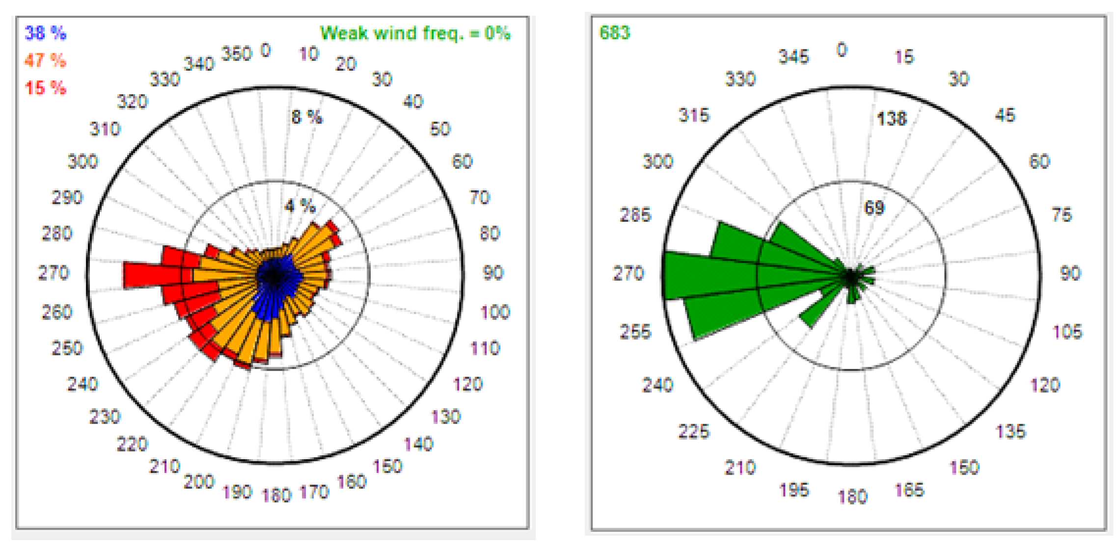
Ten years of wind speed and direction analysis are shown in Figure 2. The wind potential is analysed using data from NCDC. This analysis shows that about 90% of wind potential comes from the west, mainly during the day (not during the night).

Figure 2.
Rose of the wind speed (left) and wind potential (right).
In order to achieve specific local results, wind measurement equipment was installed near the parapet of the building, including two cup anemometers, one wind vane, and one sonic anemometer, as illustrated in Figure 3 (photograph on the left is facing the dominant winds from the west). The wind measurement data at the top and bottom cap anemometers have been analysed in Section 5.2 and then compared with LES results at the same location. A one-year measurement campaign brought enough information to characterize the wind from the west direction. The direction of the wind is depicted in Figure 1 and Figure 2 and is perpendicular to the front wall of the building. Other properties of the location are as follows:
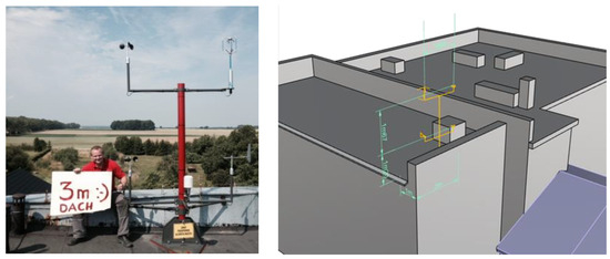
Figure 3.
Mast installation on the roof of the building: Cap and vane anemometers (left), dimensions of the mast (right).
- Turbulence intensity: 25% at the top anemometer, 41% at the lower anemometer.
- Wind shear: about 3.5.
- Flow is twisted: horizontal direction is 15° shifted from the top location to the lower location (close to the roof, flow deviates to the left).
All the local measurements have been performed by METEODYN (http://www.meteodyn.com/en), and the meteorological data have also been gathered by METEODYN during the SWIP project (http://swipproject.eu/).
3. Computational Domain
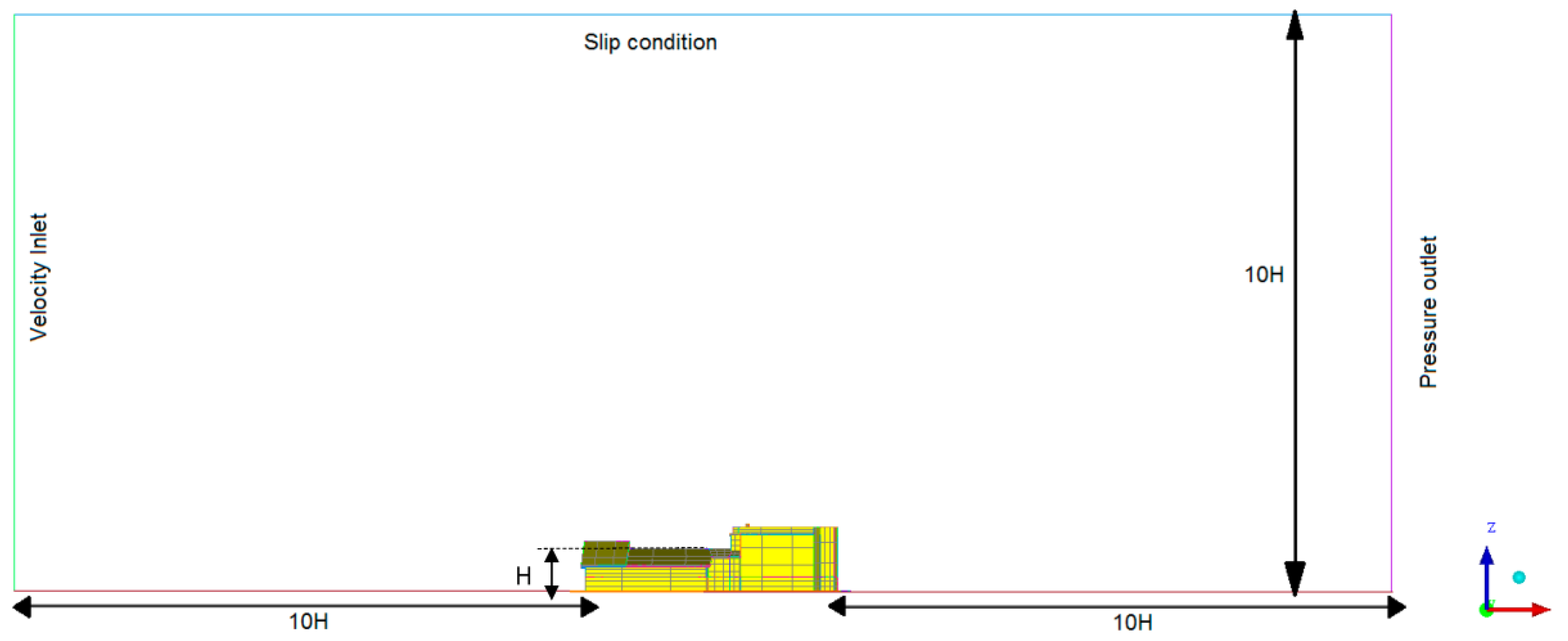
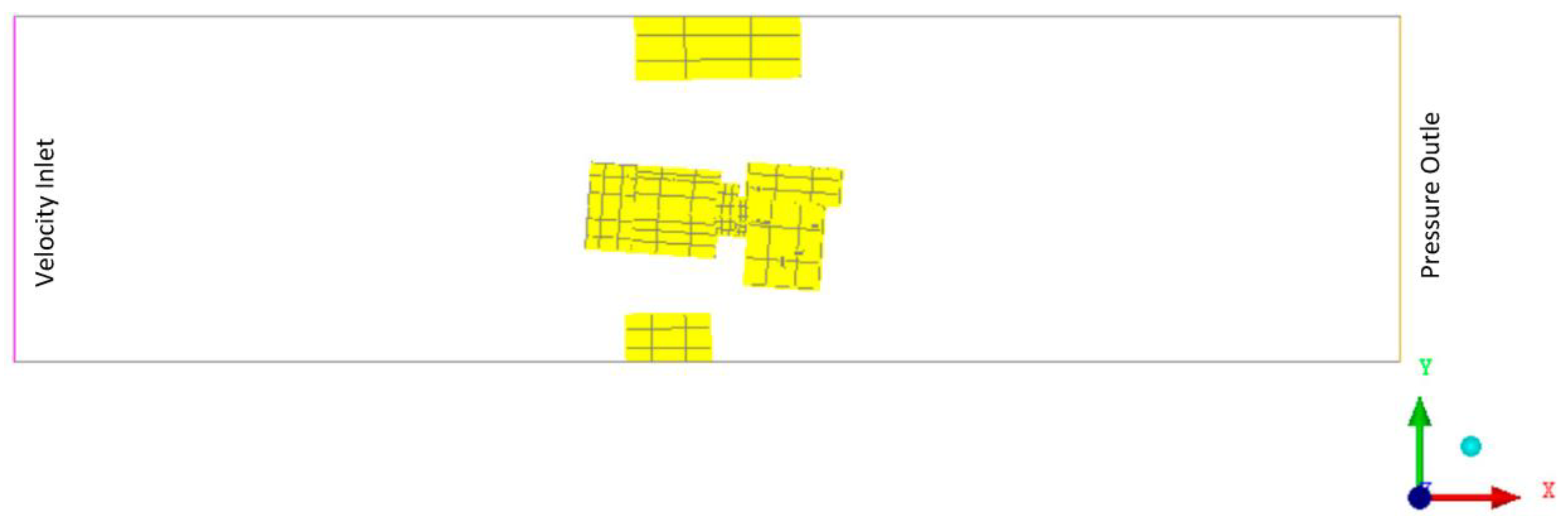
The computational domain includes the main building of interest with all its details and the two nearest buildings that are illustrated in Figure 1. Considering the wind direction, the vegetation cover was removed, as no trees were in the upstream wind. The ground was assumed flat. As discussed in the previous section, the prevailing wind direction was normal to the building’s main axis. The computational domain is depicted in Figure 4 and Figure 5.
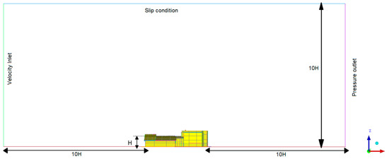
Figure 4.
A side view of the computational domain (H is the height of the building).

Figure 5.
A top view of the domain.
The top boundary condition is set at 10 H and the inlet at 10 H from the building and the outlet at 10 H from the end of the building. In this setting, H is the height of the central building’s front wall, and this is depicted in Figure 4. These are very similar to the dimensions suggested by COST (European Cooperation in the Field of Scientific and Technical Research), and [17,18,19], and are utilized by other researchers [20,21]. These dimensions are selected so that there is no reflection of the disturbance in the domain close to them. To reduce the size of the computational domain, the side boundaries pass through the middle of the neighbouring buildings. This domain will have a substantially smaller mesh size, which has no significant impact on the results.
3.1. Mesh Quality
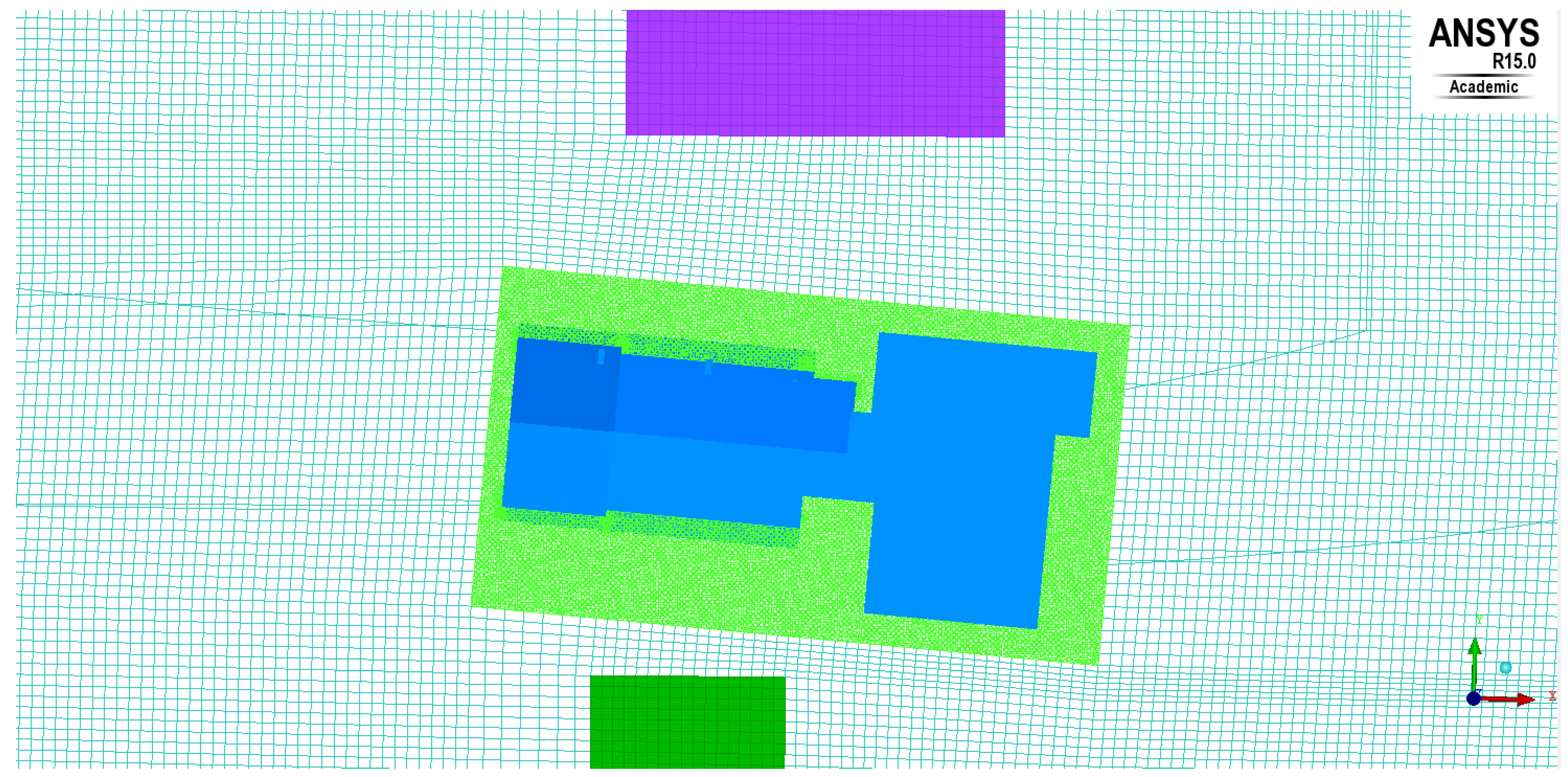
In the simulation, the domain is discretised using a hybrid mesh. An unstructured mesh is used in a rectangular area close to the central building and a structured mesh is employed in the rest of the domain. A mesh interface is defined at the connection location of the two meshes. The total number of cells in the domain is 4,481,950, where 2,110,248 cells belong to the unstructured region around the central building. To capture the complex flow pattern around the building, the grid has been refined near the building and around the rooftop. A mesh interface connects the meshing of the structured and unstructured parts. Figure 6 depicts a top view of the mesh distribution in the domain.
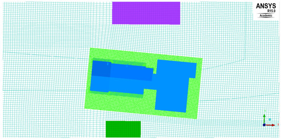
Figure 6.
A top view of the mesh.
In wind engineering applications, the grid resolution of LES cases is such a controversial issue. During grid refinement in LES, the model contribution changes as well [22]. Therefore, the smaller the grid size the larger the range of the eddy scales resolved by the LES model. Consequently, the grid independency of the RANs techniques do not apply here.
For most applications of LES, the grid resolution in the regions close to the solid wall is limited by the filtering length, i.e., the Kolmogorov integral length scale. The microscopic scales, which mainly occur in the sub-grid scales of the domain, are modelled. Therefore, the mesh density can be reduced as far as the numerical technique supports. The main criteria for checking the grid quality is through the LES index of Quality (LES_IQ) [23,24] and is a measure of the rate of the resolved part of the turbulent kinetic energy to the total kinetic energy :
where , and and are the contribution of the SGS and numerical dissipation, respectively. There are some debates about the above equation, as, in some cases, a higher value for has been reported on a coarser mesh [24,25]. Celik suggested the following formula, where LES_IQ is required to be below 1 [24]:
As the calculation of is difficult and out of the scope of this research, we used simplified criteria proposed by Pope [23], suggesting that if 80% of the turbulence energy is resolved, the grid is sufficiently fine. Based on our simulations of modelled and resolved kinetic energy, the maximum modelled kinetic energy was much smaller than the resolved kinetic energy, thus indicating that the Pope criteria were met.
3.2. Boundary Conditions
The boundary conditions are illustrated in Figure 4. The buildings and the ground surfaces are defined as a wall. A logarithmic velocity profile is imposed at the inlet:
where is the friction velocity, is the height of the zero plane above the ground, and is the surface roughness length parameter. A more general form of this equation is discussed in [14]. The inlet velocity at the central building height is assumed to be equal to the most frequent velocity according to the data provided by METEODYN (http://meteodyn.com/).
The turbulence intensity and the kinetic energy and dissipation rate also have been calculated and implemented as a profile in the inlet. All these boundary conditions are used for the RANS calculations. The RANS calculations will later be used initializing the LES through inflow generation, which is covered in Section 4.2.
4. Numerical Details
The large eddy simulation of the computational domain was performed using the commercial CFD package ANSYS Fluent. The convection terms in the momentum equations were discretized using a bounded central-differencing scheme, which has an accuracy of the order between one and two, together with a second-order technique for the pressure term. Also, a second-order implicit time integration technique is used. This technique has been shown to be capable of providing more stable solutions for unsteady problems [26]. Time steps of 0.01 s were used during the running of the LES. This time step resulted in local Courant numbers in the domain, which are less than 2.4, and these values for Courant number were small enough to generate stable numerical results. The coupling between the velocity and pressure was through the non-iterative pressure implicit scheme with the splitting of operators, i.e., PISO, which has been widely utilised in similar research [14,20], and a bounded central difference was used to discretizing the momentum convective terms which prevent unphysical oscillations [27]. In order to start the LES, the solution are initialized from the steady-state RANS results. In this work, a realizable k- turbulence model is used for the RANS calculations, and LES simulations were started after converged RANS results were obtained. The sample data were captured after 8000 time steps of running an initialized LES solution. This is equivalent to 2.26 mean flow residence time, ( where is the streamwise dimension of the computational domain). The sample data were captured every 1000 time steps for a total time of 480 s, . The computation was performed using the high performance computing facilities (HPC) of the University of Sheffield. In total, 20 CPUs were used in parallel for the simulation.
4.1. Wall Function and SGS Model
To represent the near-wall structures accurately, the first grid point must be located at z+ < 1. Alternatively, approximate boundary conditions or wall models may be used in LES. When the grid is not fine enough to resolve the gradients near the wall, a wall function is used to approximate the flow in a very small region close to the solid bodies. This allows us to place the first node at z+ ≈ 30–200. The wall functions are ideal for wind engineering problems where most of the turbulence energy is provided by the larger scales in the domain.
In this paper, the Werner–Wengle wall function is utilized, which proved a power-law profile to return an estimation of the instantaneous wall shear stress for a given velocity at the wall nearest node [27]. The Werner–Wengle function has been used for complicated applications of separated flows and has been shown to be the most effective estimator that can replace the highly resolved LES near walls [28]. The combination of the subgrid scale and the Werner–Wengle near-wall approximation was very effective at the moderate z+ values [28]. During the LES calculation, apart from near-wall solutions, filtering was applied to the Navier–Stokes equations. The residual (subgrid) unfiltered part of the flow are modelled through a Sub-Grid-Scale (SGS) model. More information about different SGS models and their physical interpretations is available in previous publications [29,30]. The dynamic Smagorinsky Lily model is used for the current application [31,32]. This model is an improved version of the standard Smagorinsky model [33] and had an improved transfer of the kinetic energy to the sub-grid, which also has been successfully applied to numerous similar applications [20,26,34].
4.2. Inflow Generation
The Smirnov random flow generation method (RFG) is utilized to initialize velocity turbulence fields in the domain [12]. This technique was incorporated in the Fluent software, defined as the Spectral Synthesizer [35]. The most important advantage of the Smirnov method over other inflow generation methods is that it is divergent-free [4,35]. Also, the technique is capable of generating inhomogeneous and anisotropic turbulence. The velocity fluctuations were introduced to the domain through a series of Fourier harmonics, and the modelled turbulence spectrum is represented by:
where is the wave number. The Smirnov method receives the correlation tensor of the original flow field and information on the integral length scale of the turbulence as inputs. These quantities could be estimated using the Reynolds stress terms from previous RANS computations or experimental data [12]. There are several ways to provide inputs for the Spectral Synthesizer techniques. One of the most realistic ways is to define the turbulence kinetic energy and dissipation rate profiles at the inlet [36]:
where is the vertical profile of turbulence intensity, is the mean velocity at the inlet, and are the turbulence kinetic energy and dissipation rate per units of mass, respectively, is a constant equal to 0.09, is the distance to the wall, and is von Karman constant.
4.2.1. Turbulence Intensity and Reduced Length Scale
The values of the turbulence intensity and integral length scale for the above calculations were normally obtained from experimental measurements, i.e., Section 2, at the location of the inlet. The integral length scale is the largest Eddy motions in a turbulent flow. The atmospheric integral length scales from measurements are quite large (38~60 m). Implementing these length scales is only possible in mesoscale simulations [2]. Therefore, following the method of Jensen et al. [37] and Berg et al. [2] for scaling the length scale of small hill terrain, we estimated a smaller length scale of 7 at the inlet. As a direct consequence of implementing a scaled length scale at the inlet, the generated length scale at the building roof is not expected to be the same as the measurements. We will investigate the effect of considering these reduced length scales in the generated turbulence in the results section. The turbulence intensity profile, which was implemented at the inlet, is shown in Figure 7. The turbulence intensity increased at a close distance to the wall, and then it decreased with height. All calculations and estimations in this section were based on a neutral atmospheric condition.
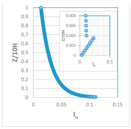
Figure 7.
Turbulence Intensity profile at the inlet of the computational domain. The top box shows the changes in a zoomed area close to the ground.
5. Results and Discussion
Simulated inflow turbulence, as well as mean velocity profiles along with simulated and measured wind energy spectra at the top of the building, are discussed in Section 5.1 and Section 5.2, respectively. The analysis of the wind data is performed in exactly the same location as the ones that are discussed in Section 2. The flow field features are depicted in Section 5.3, and, finally, the effects of the neighbouring buildings and a proposed location for a turbine installation are illustrated in Section 5.4.
5.1. Inflow Turbulence
To study the effectiveness of the spectral synthesizer, the power spectrum of generated turbulence is calculated and validated with the von Karman wind spectra. The streamwise component of the von Karman formulation is described as follows [10,21]:
where is the fluctuating term of the streamwise velocity, is the frequency, and is the variance of the streamwise velocity. Also, in this formulation, is the non-dimensional (reduced) frequency:
where is the integral length scale, and is the local average velocity. Equation () is suitable for isotropic turbulence and neutrally stratified flows.
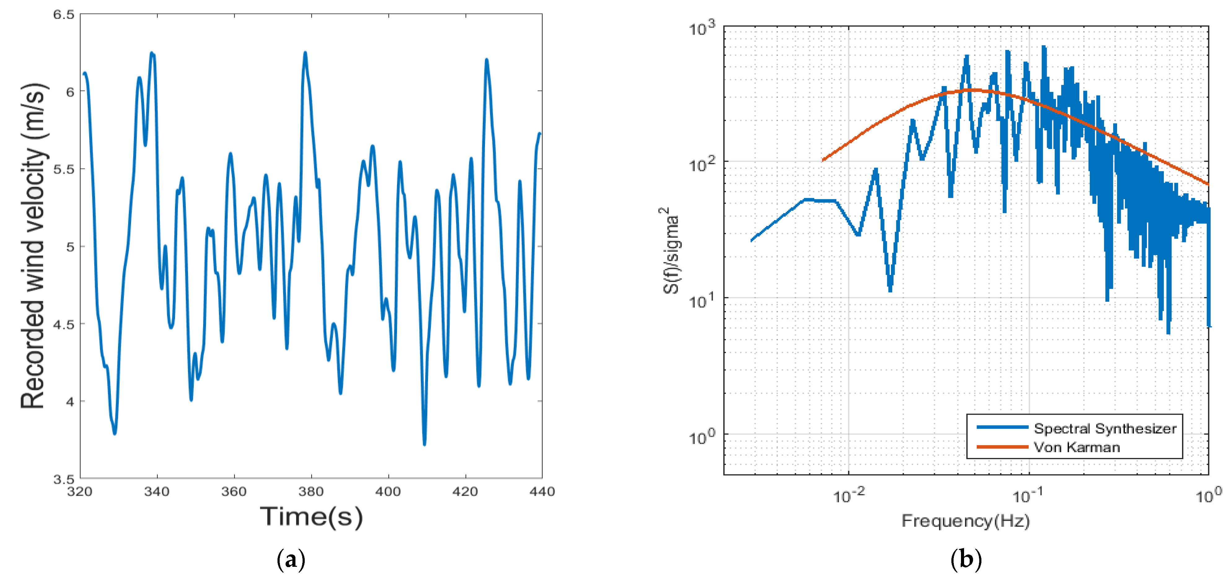
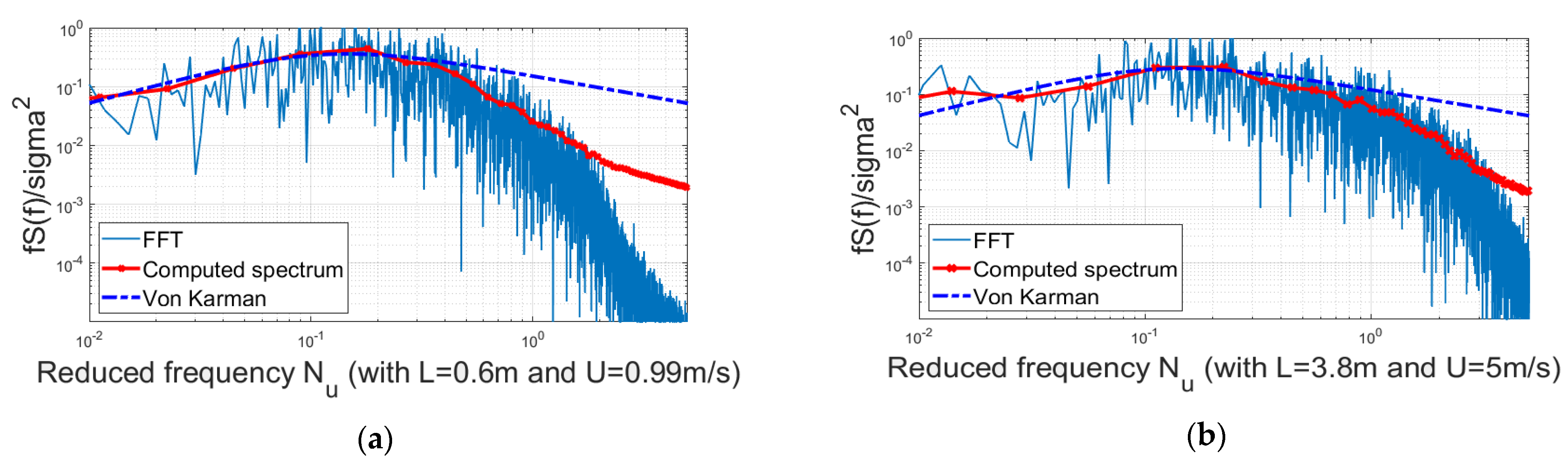
LES simulated wind data and power spectral density are evaluated in Figure 8 for a point at 1 H downstream of the inlet. The energy spectrum from the Spectral Synthesizer covers a range of high-frequency as well as low-frequency turbulences. The slope of the energy spectrum follows the von Karman spectrum in the high- and low-frequency ranges. At the very end of the high-frequency range, the LES slope becomes slightly steeper; nevertheless, the difference is small.
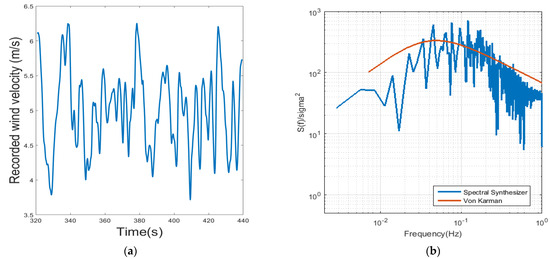
Figure 8.
Wind velocity history (a) and power spectral density (b) at x = 1.0 H, y = 0.0, and z = 1.0 H from the inlet at the centre of the spanwise direction. The ground is at z = 0.0. The average velocity of 4.0 m/s and length scale of 10 m have been used for von Karman calculations.
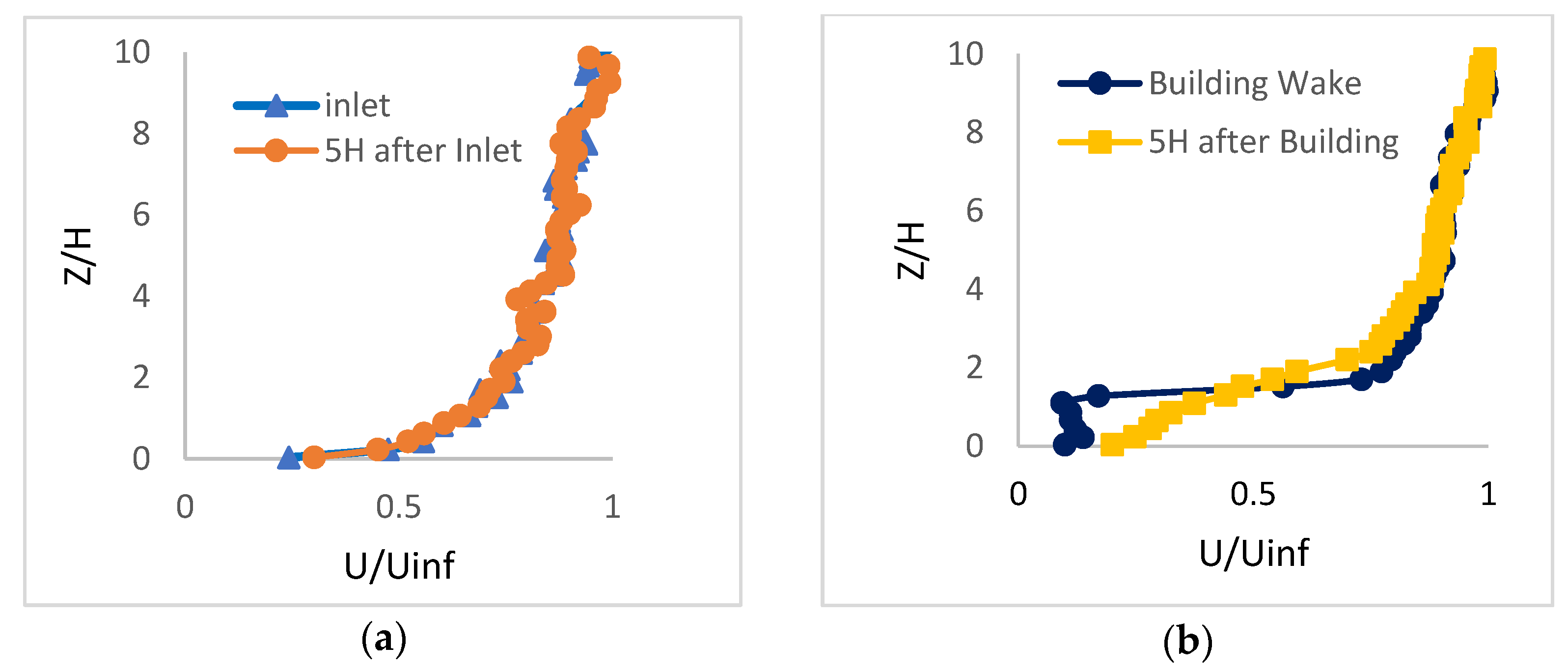
Figure 9a,b show mean wind structures at the inlet and three other streamwise locations, i.e., 5 H downstream inlet and in a leeward location of the building where the wake occurs and 5 H after building. The upstream location 5 H is midway between the inlet and the central building. As there is no obstacle between the inlet and 5 H streamwise locations, it is expected that the mean velocity remains the same. According to Figure 9a, the mean wind profile is preserved well in the domain, ahead of the building. Despite the excellent agreement, there is a difference between the inlet and 5 H location that occurs due to the inevitable damping of some high-frequency oscillations in the streamwise location. This will be discussed further in Section 5.2. Figure 9b depicts the mean wind profile at the leeward side of the building and 5 H after the building. The wake flow and the recirculation zone are the major sources of difference in mean velocity profiles of Figure 9b and will be discussed in more detail in Section 5.3. The wind profile on the leeward side recovers from the wake flow, moving further away from the building at the 5 H distance after the building; there is a change in the mean velocity profile, as shown in Figure 9b.

Figure 9.
Mean wind profile comparisons (a) between inlet and building, (b) in the building wake.
5.2. Validation of the LES Results against Measurement Data
Wind data are recorded for LES and measurements at the location of two cup anemometers, which are depicted in Figure 3. The upper cup location is defined at Point 1, and the lower cup is defined at Point 2. Point 2 is, therefore, closer to the parapet of the front building and so is more influenced by the vortices near the edge of the wall. Point 1 is 1.60 m higher than Point 2 but has the same spanwise and streamwise locations.
5.2.1. Energy Spectrum
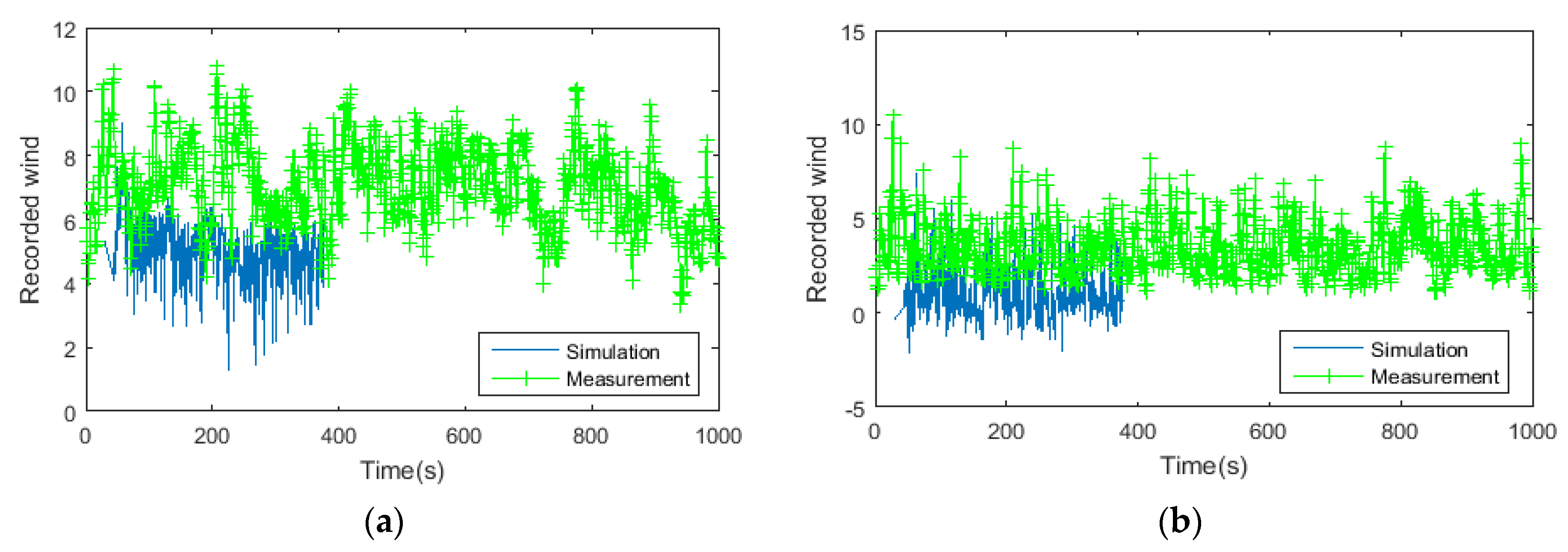
Figure 10 shows the wind history at two points on the top of the building. The points are illustrated in Section 2 and also shown in Figure 3. The data from the measurements are recorded at a frequency of 1.0 Hz for 2 h, and the frequency of sampling for LES is 0.1 kHz for 400 s.
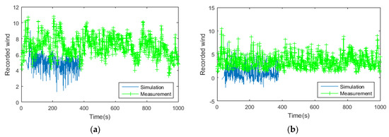
Figure 10.
Simulated wind from the spectral synthesizer and measured wind (m/s) in the streamwise direction at (a) Point 1 and (b) Point 2.
Simulated time series exhibit variations much faster than the measurements, and this is due to two main reasons. The first one concerns the sampling frequencies, which differ by a factor of 10 so that the simulated data can contain higher frequencies than the measurement data. The second reason comes from the reduction in the turbulent length scale, which is much smaller in the simulation (7 m instead of ~60 m). Nevertheless, the order of magnitude of the mean wind speed is similar from the simulation to the measurement: most of all, the reduction from Point 1 to Point 2 is correctly captured in the simulation results.
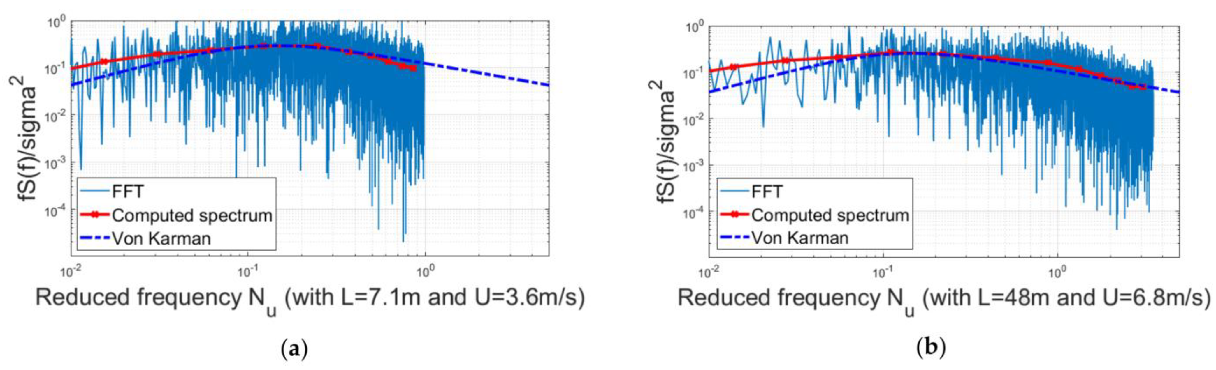
Figure 11 and Figure 12 show the energy spectrum for the measured and LES results at two points. The energy spectrum is computed from the fast Fourier transform and compared with the von Karman wind spectra of Equation () for the measurements and the Spectral synthesizer method. The length scale used for the calculation of the reduced frequency is described in the next section.
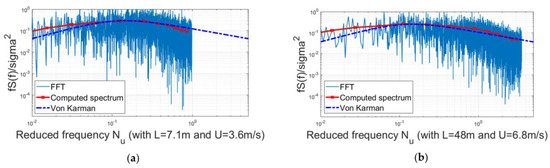
Figure 11.
Energy spectrum from the time series at Point 1 for (a) measurements and (b) Spectral synthesizer.
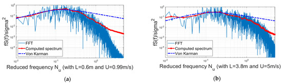
Figure 12.
Energy spectrum generated from the time series data at Point 2 for (a) measurement and (b) Spectral synthesizer.
At Point 1, high frequencies perfectly follow the von Karman spectrum in the measurement, whereas there is a decay in the high-frequency range in the Spectral synthesizer results. This can be linked to two factors: the first one is the inherent cut-off in the Spectral synthesizer method. The second factor is a predictable damping of the high frequency in the domain, not only between the inlet and the building (Figure 12) but specifically at the location of the measurements, which is exposed to the velocity gradients of the parapet and the wake region in front of the building, and this will be shown later. This could be difficult for the Spectral Synthesizer to deal with the flow in this region, which is highly anisotropic and disturbed. Apart from the Spectral Synthesizer method, this deviation is partly due to the effect of the SGS [4] or the restriction of the mesh resolution [21,38] and a similar behaviour has been reported by Huang et al. [10].
At Point 2 of Figure 12a, the spectrum stops at a reduced frequency of 1, which is quite low. This is due to three factors: (i) the limited sampling frequency of the measurements (1 Hz), (ii) the small wind speed at this point (wind is reduced close to the parapet), and (iii) the utilised turbulent length scale at the inlet. The fact that the cutting frequency appears to be more at Point 2 than at Point 1 shows that the reduction in length scale exceeds the reduction in the mean wind speed.
Away from the high-frequency region, the slopes of measurement and simulated results follow the theoretical values perfectly well in the low-frequency range. The energy spectrum peaks at the integral length scale, which is very similar to the LES and measurements plots at both points. This will be investigated and further confirmed in Section 4.2.1 and Section 5.2.2 The calculated spectrum, i.e., the red lines in Figure 11 and Figure 12, slightly overestimates the theoretical values for the measurements in the low-frequency range.
5.2.2. Turbulence Length Scale
As we discussed in Section 4.2, the length scale that is employed at the inlet of the LES computational domain is much smaller than that of the real wind conditions according to the measurements. This is a limitation for most wind simulation cases. In order to study the effect of the inlet condition on the generated length scales of the wind on the roof, the integral length scale of the wind is calculated for the measured and simulated wind using the following equation [39]:
where is the energy spectrum of the turbulence flow field, which is calculated from Section 5.2.1. Table 1 illustrates the integral length scales calculated using Equation (9) for the two points of Figure 3. This table shows the ratio of the length scales to the inlet integral length scale, which is 7 ( for LES and 60 ( for measurement. The first and second columns represent the reduced length scale values for the LES and measurements, respectively. As expected, the length scale at both points was decreased at the rooftop due to the presence of the building. Comparing Points 1 and 2, the length scale decreased remarkably at Point 2 for both measurement and LES results. Although there is less than a meter difference between the heights of the two points, both the measurement and simulation show a significant reduction in the values. The significant point about these results is that the LES and measurement values are very similar. This confirms that although the considered inlet length scale is more than 8 times smaller than real wind data, the resolved length scales and their spatial variations at these points are very similar to the measurement values, and they can be scaled up at any location of interest inside the domain for the real length scale predictions. Accordingly, by repeating this simulation for similar problems, then it is possible to obtain an estimation of the real wind turbulence length scales, where no measurement data are available.

Table 1.
Comparison of the LES results with the measured data.
5.3. Turbulent Flow Fields
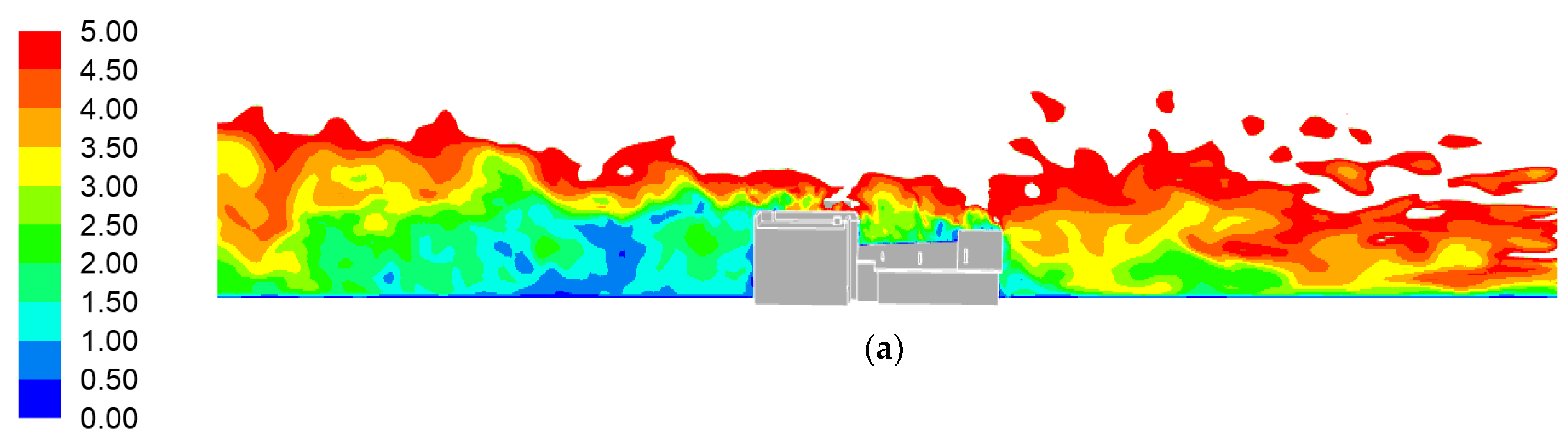
In order to examine the quality of the generated inflow in the streamwise direction, instantaneous velocity components are calculated on a vertical and a horizontal plane in the computational domain. Figure 13 depicts the contours of the velocity magnitude in the streamwise direction in the solution domain in the side and top views. In the upstream region, and close to the inlet of the domain, a reasonable amount of velocity fluctuations is generated. However, the turbulence structures are a little bulky, and not many scales are observed in the domain. This can be also observed in Figure 13b. However, as the turbulent flow develops further, it becomes finer, and more visible features are added to the structure. The building influences the downstream flow over a reasonable range, which is almost equal to the length of the building before the wake flow disappears. The wake flow behind the neighbouring buildings does not extend as long as the central building. The reason for that is the strong acceleration of the flow in the corridor between the buildings and towards the sides that eliminates the wakes soon after they form.

Figure 13.
Instantaneous velocity magnitudes (m/s) at (a) Y = 0 vertical and (b) Z = 0.25 H horizontal planes.
5.4. Suggested Location for a Small Roof-Mounted Wind Turbine
The key characteristics of the wind regarding the location of a roof-mounted turbine are uniformity and maximum potential wind. To determine the location for wind turbine installation, we performed a comprehensive analysis of the wind flows around the central building and especially on the roof. As depicted in Figure 6, the neighbouring buildings are not in the same streamwise locations as the central building. The right building is the first building that appears in the streamwise direction, then the central building, and, finally, the left building. In order to study the effect of the neighbouring buildings, a cut plan is defined in the domain that passes through all three buildings, as illustrated in Figure 14.
Figure 14.
Cut plane introduced through the central building and the two neighbouring buildings.
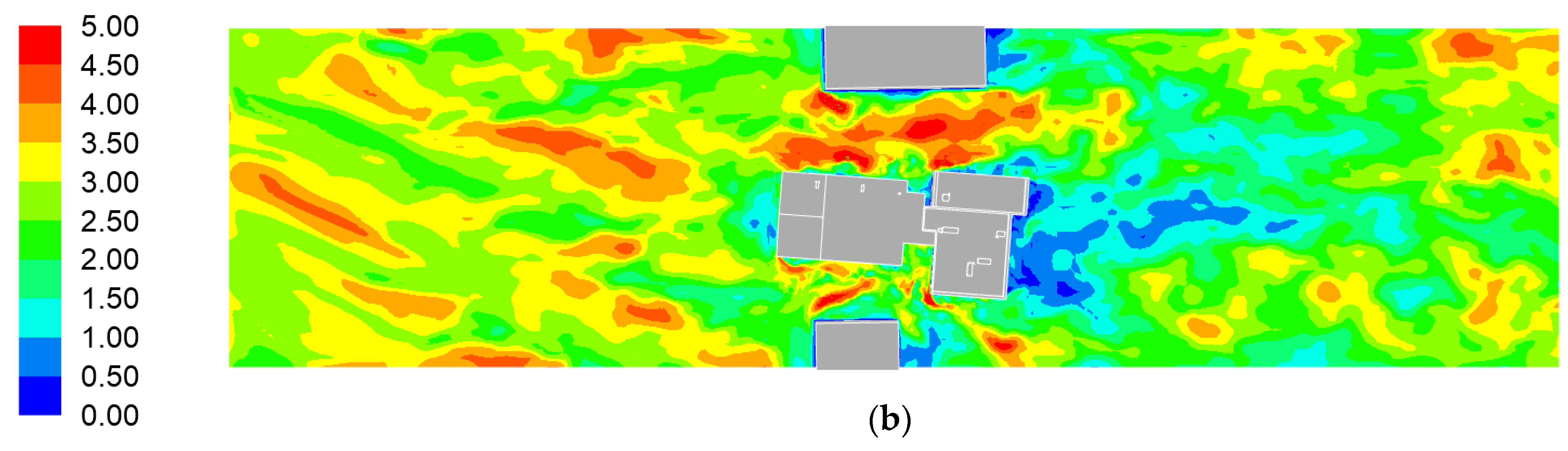
The path lines of the instantaneous velocity magnitude for this cut plan are shown in Figure 15, and the effect of the neighbouring buildings is presented in this plot as well. The wake next to the left wall developed stronger downstream, and this region was about 50% wider than the region between the central and right building, where the wind was faster. Therefore, no large vortexes were depicted near the right wall, and the wind was significantly stronger on the right gable roof compared to the left side.

Figure 15.
Cut plane 2 passing through the central and two neighbouring buildings: instantaneous velocity magnitude path lines (m/s).
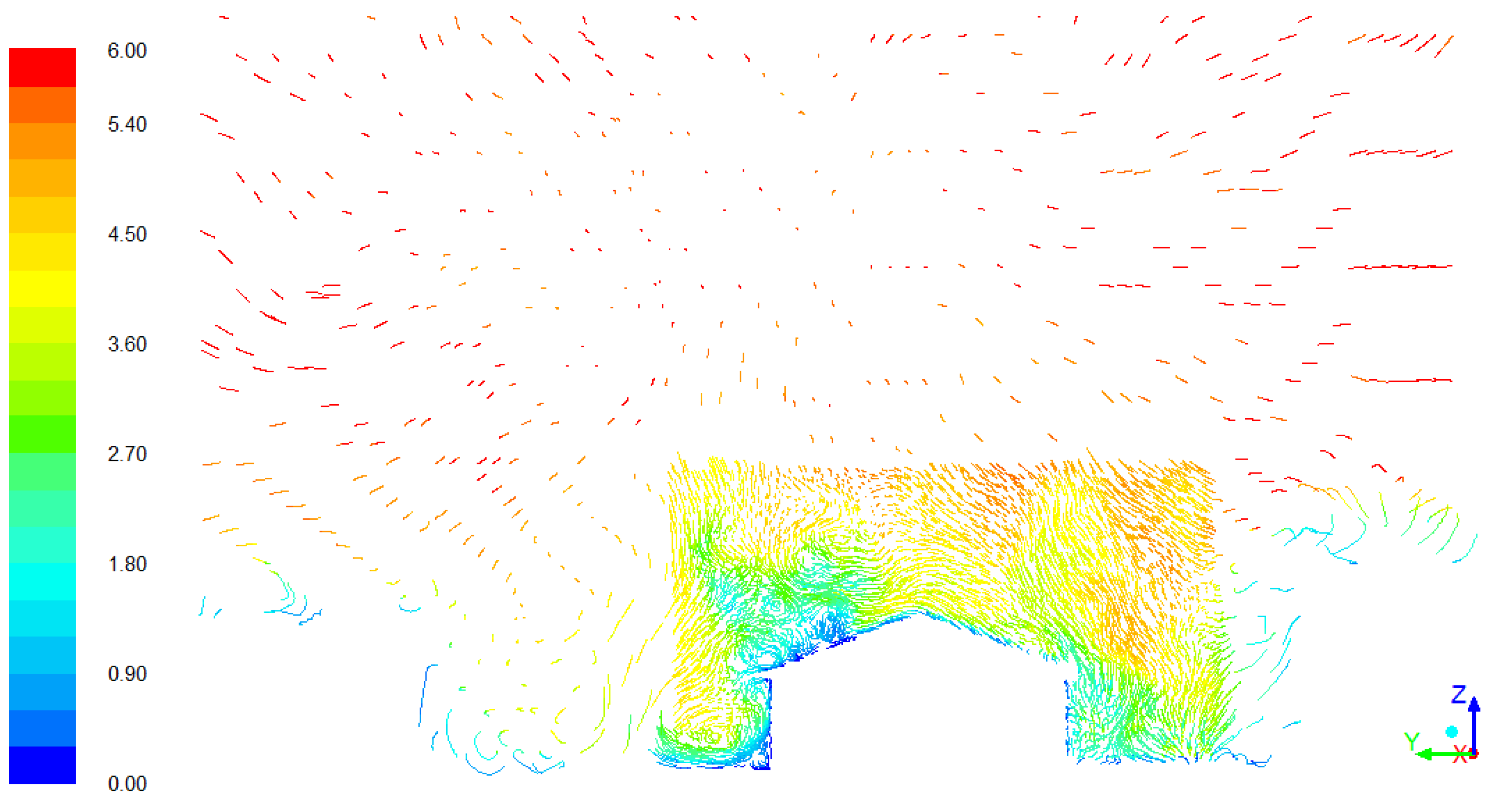
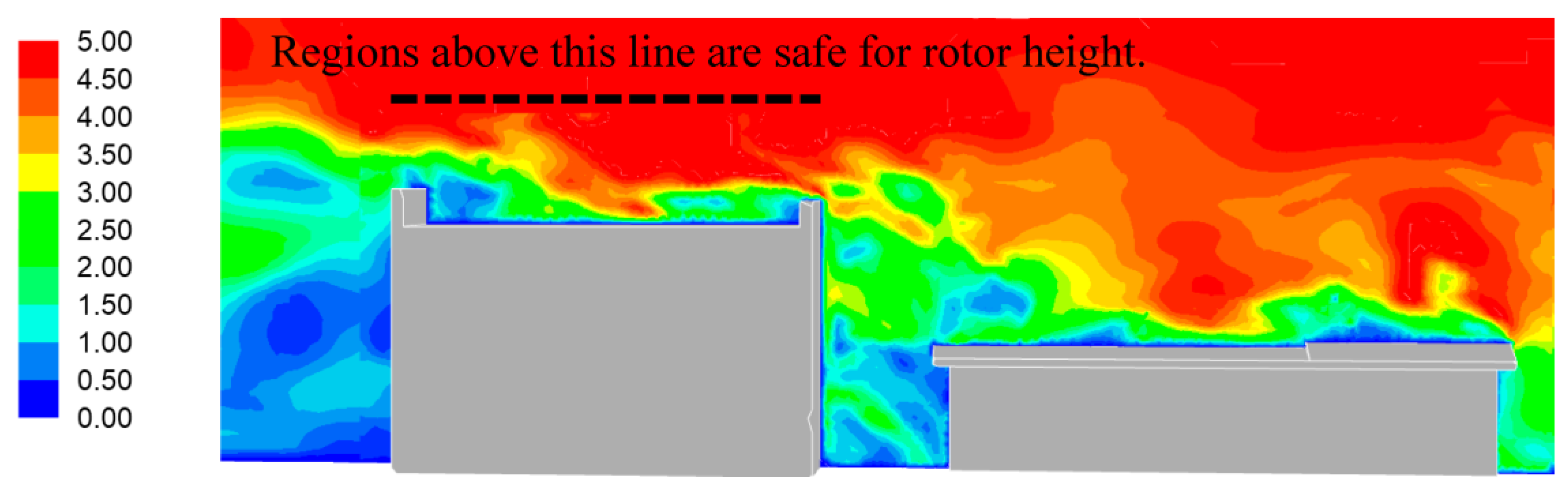
A streamwise view of the velocity contour at the left side of the central building is illustrated in Figure 16. The cut plan at the front part passes the location of the measurement instrument. The roof flow is clearly less disturbed at this location compared with the gable roof. The wind speed at this location is high as well, so this location is potentially suitable for a roof-mounted small wind turbine installation. Another advantage is that the roof is flat at this location, and, therefore, the installation is also much easier compared to the gable roof.
Figure 16.
Streamwise instantaneous velocity magnitude of the central building roof.
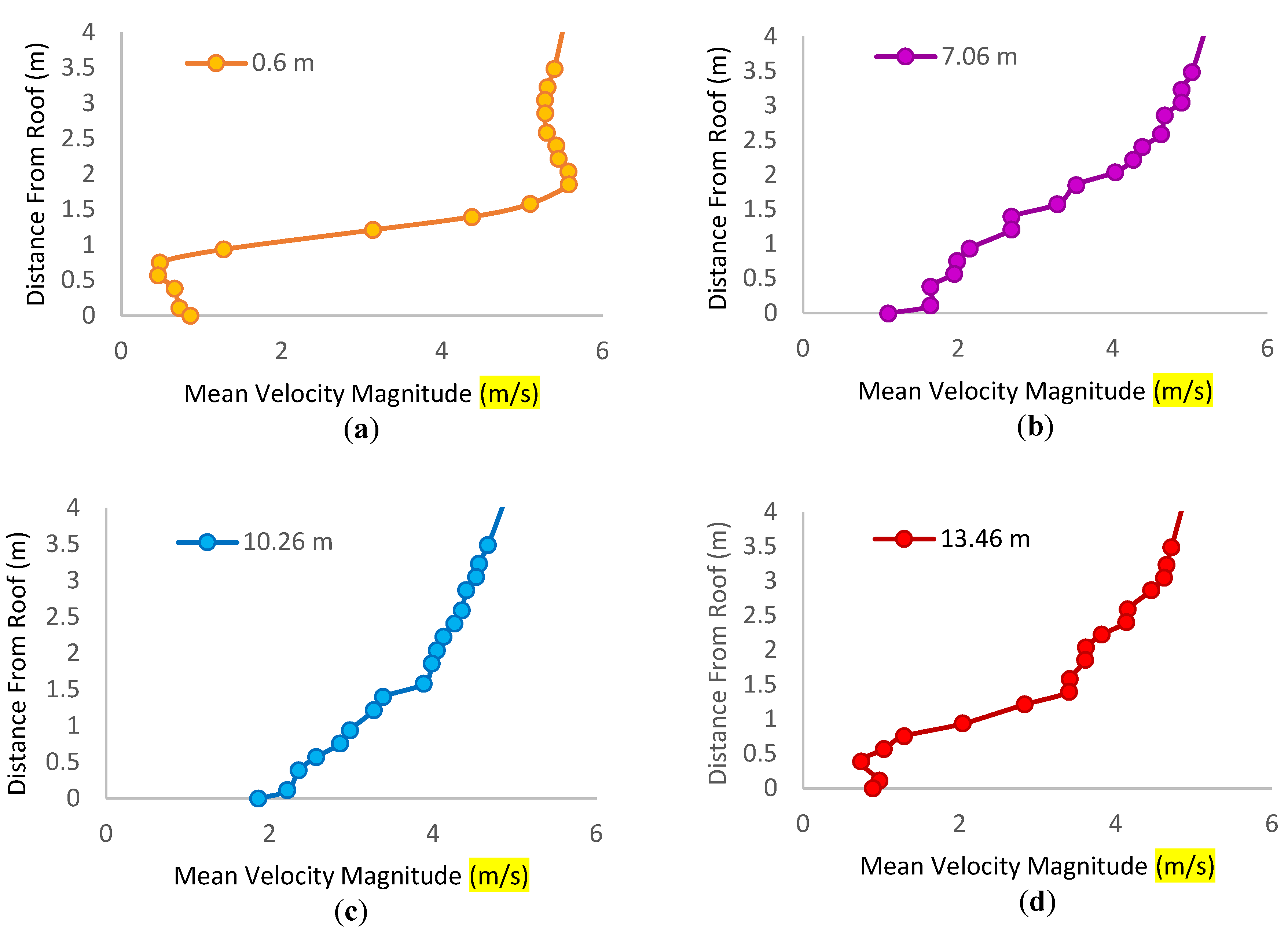
In the regions close to the rear and front parapets, a wake is formed, and the wake is stronger near the rear parapet. The velocity contours tend to become uniform at about 3 m away from the roof. These instantaneous observations are supported by the mean velocity profiles of Figure 17a–d. The velocity profiles present four streamwise locations on the flat roof. The distances of the velocity profiles are measured from the front parapet. The velocity profile of Figure 17a predicts a wake flow near the front parapet. The kinetic energy of the wind flow dominates the vortices in the velocity profiles of Figure 17b,c. Again, moving towards the rear parapet, another wake is formed, and we can see these effects in Figure 17d. Most of these disturbances approximately diminish at 0.3 H from the rooftop, where H is the height of the front view of the building (refer to Figure 4). Therefore, to avoid turbulence at this location, the wind turbine mast height should be about 0.3 H above the roof.

Figure 17.
Mean velocity profiles: (a) 0.6 m from the parapet, (b) 7.06 m from the parapet, (c) 10.26 m from the parapet, and (d) 13.46 m from the parapet.
6. Conclusions
In this paper, the reliability of a reduced integral length scale for the inflow generation of LES was studied. During this investigation, we showed that there was a meaningful relationship between the simulation and measurement results. We performed this study on a practical case, which was a low-rise building and its two simplified neighbouring buildings. LES was implemented in ANSYS/Fluent using spectral synthesizer inflow generation. Also, a combination of the Werner–Wengle wall function for the near wall treatment and the dynamic Smagorinsky Lily method for the sub-grid scale modelling was used.
We carried out field measurements at the location of interest. The local wind data were measured using two cup anemometers on the roof of the building, and the wind data were analysed to obtain the real energy spectrum and length scale of the location.
The length scale at specific points on the roof of the building was calculated using measurement and simulated data, and the simulation energy spectrum and length scales were validated with local measurements. While the inlet turbulence length scales were different, we could obtain a very good agreement between the generated length scale from the LES simulation and the local measurements when they were scaled with their corresponding inlet value. This was a very promising result, as, in most cases, implementing a real length scale to the computational domain was impractical due to the domain dimension requirement.
The main flow features around the central low-rise building and the vortex shedding from the sidewalls were studied, and the effect of the neighbouring buildings was investigated. The results clearly illustrated that the neighbouring buildings could cause a high level of wind speed on the roof for constructions of similar heights. In the case of a wind turbine, this could be an advantage, and these regions were potentially suitable for wind turbine installations. Based on the simulation results, the best potential location for the installation of a small vertical-axis wind turbine was proposed.
Author Contributions
Conceptualization, A.S.; Methodology, A.S. and J.B.-G., Software, A.S.; Validation, A.S. and J.B.-G.; Formal Analysis, A.S.; Investigation, A.S.; Resources, J.B.-G.; Writing—Original Draft Preparation, A.S.; Writing—Review and Editing, A.S., J.B.-G., L.M. and D.I.; Visualization, A.S. and J.B.-G.; Supervision, L.M., D.I. and M.P.; Project Administration, A.S. and L.M.; Funding Acquisition, M.P. All authors have read and agreed to the published version of the manuscript.
Funding
This paper is part of an EU Horizon 2020 project “New innovative solutions, components, and tools for the integration of wind energy in urban and peri-urban areas” (acronym SWIP, project no. 608554), http://swipproject.eu/.
Data Availability Statement
Not applicable.
Acknowledgments
We thank Leonardo Subias, the coordinator of the SWIP project of the Circe Company (www.fcirce.es), for their support during the project.
Conflicts of Interest
The authors declare no conflict of interest.
References
- Nozu, T.; Tamura, T. LES of turbulent wind and gas dispersion in a city. J. Wind Eng. Ind. Aerodyn. 2012, 104, 492–499. [Google Scholar] [CrossRef]
- Berg, J.; Mann, J.; Bechmann, A.; Courtney, M.S.; Jørgensen, H.E. The Bolund Experiment, Part I: Flow over a steep, three-dimensional hill. Bound.-Layer Meteorol. 2011, 141, 219–243. [Google Scholar] [CrossRef]
- Bechmann, A.; Sørensen, N.N.; Berg, J.; Mann, J.; Réthoré, P.E. The Bolund Experiment, Part II: Blind comparison of microscale flow models. Bound.-Layer Meteorol. 2011, 141, 245–271. [Google Scholar] [CrossRef]
- Baba-Ahmadi, G.R.H.; Tabor, M. Inlet condition for large eddy simulation: A review. Comput. Fluids 2010, 39, 553–567. [Google Scholar]
- Spalart, P.R.; Leonard, A. Direct Numerical Simulation of Equilibrium Turbulent Boundary Layers; Springer: Berlin/Heidelberg, Germany, 1985; Available online: https://link.springer.com/chapter/10.1007/978-3-642-71435-1_20 (accessed on 3 November 2015).
- Lunda, T.S.; Wu, X.; Kyle, D.; Squires, K.D. Generation of Turbulent Inflow Data for Spatially-Developing Boundary Layer Simulations. J. Comput. Phys. 1998, 140, 233–258. [Google Scholar] [CrossRef]
- Yoshida, T.; Takemi, T.; Horiguchi, M. Large-Eddy-Simulation Study of the Effects of Building-Height Variability on Turbulent Flows over an Actual Urban Area. Bound.-Layer Meteorol. 2018, 168, 127–153. [Google Scholar] [CrossRef]
- Jarrin, N.; Benhamadouche, S.; Laurence, D.; Prosser, R. A synthetic-eddy-method for generating inflow conditions for large-eddy simulation. Int. J. Heat Fluid Flow 2006, 27, 585–593. [Google Scholar] [CrossRef]
- Zhang, D.; Zheng, A. Improvement of inflow boundary condition in large eddy simulation of flow around tall building. J. Eng. Appl. Comput. Fluid Dyn. 2012, 6, 633–647. [Google Scholar] [CrossRef]
- Huang, S.H.; Li, Q.S. A new dynamic one-equation subgrid-scale model for large eddy simulations. J. Numer. Method Eng. 2010, 81, 835–865. [Google Scholar] [CrossRef]
- Jarrin, N. Synthetic Inflow Boundary Conditions for the Numerical Simulation of Turbulence. Ph.D. Thesis, University of Manchester, Faculty of Engineering and Physical Science, Manchester, UK, 2008. [Google Scholar]
- Smirnov, A.; Shi, S.; Celik, I. Random flow generation technique for large eddy simulations and particle-dynamics modeling. J. Fluids Eng. 2001, 123, 359–371. [Google Scholar] [CrossRef]
- Luo, Y.; Liu, H.; Huang, Q.; Xue, H.; Lin, K. A multi-scale synthetic eddy method for generating inflow data for LES. Comput. Fluids 2017, 156, 103–112. [Google Scholar] [CrossRef]
- Vasaturo, R.; Kalkman, B.; Blocken, B.; van Wesemael, P.J.V. Large eddy simulation of the neutral atmosphere boundary layer: Performance evaluation of three inflow methods for terrains with different roughness. J. Wind Eng. Ind. Aerodyn. 2018, 173, 241–261. [Google Scholar] [CrossRef]
- Botha, J.; Shahrokhi, A.; Rice, H. An implementation of an Aeroacoustics Predication Model for Broadband noise from A Vertical Axis Wind Turbine Using a CFD informed Methodology. J. Sound Vib. 2017, 410, 389–415. [Google Scholar] [CrossRef]
- ANSYS FLUENT Theory Guide; Release 15; ANSYS Inc.: Canonsburg, PA, USA, 2013.
- Tominaga, Y.; Mochida, A.; Yoshie, R.; Kataoka, H.; Nozu, T.; Yoshikawa, M.; Shirasawa, T. AIJ guidelines for practical applications of CFD to pedestrian wind environment around buildings. J. Wind Eng. Ind. Aerodyn. 2008, 96, 1749–1761. [Google Scholar] [CrossRef]
- Franke, J.; Hellsten, A.; Schlünzen, H.; Carissimo, B. Best Practice Guideline for the CFD Simulation of Flows in the Urban Environment; University of Hamburg, Meteorological Institute, Centre for Marine and Atmospheric Sciences: Hamburg, Germany, 2007. [Google Scholar]
- Franke, J. Recommendtion of the COST action C14 on the use of CFD in predicting pedestrian wind environment. J. Wind Energy 2006, 108, 529–532. [Google Scholar]
- Huang, S.H.; Li, Q.S.; Wu, J.R. A general inflow tturbulence generator for large eddy simulation. J. Wind Eng. Ind. Aerodyn. 2010, 98, 600–617. [Google Scholar] [CrossRef]
- Daniels, S.J.; Castro, I.P.; Xie, Z.T. Peak loading and surface pressure fluctuations of a tall model building. J. Wind Eng. Ind. Aerodyn. 2013, 120, 19–120. [Google Scholar] [CrossRef]
- Freitag, M.; Klein, M. An improved method to assess the quality of large. J. Turbul. 2006, 7, 1468–5248. [Google Scholar] [CrossRef]
- Pope, S.B. Turbulent Flows; Cambridge University Press: Cambridge, UK, 2000. [Google Scholar]
- Celik, Z.N.; Cehreli, I.; Yavuz, I.B. Index of resolution quality for Large Eddy Simulations. J. Fuilds Eng. 2005, 127, 949–958. [Google Scholar] [CrossRef]
- Gousseau, P.; Blocken, B.; van Heijst, G.J.F. Quality assessment of Large-Eddy Simulation of wind flow around a high-rise building: Validation and solution verification. Comput. Fluids 2013, 79, 120–133. [Google Scholar] [CrossRef]
- Huang, S.; Li, Q.S.; Xu, S. Numerical evaluation of wind effects on a tall steel building by CFD. J. Constr. Steel Res. 2006, 63, 612–627. [Google Scholar] [CrossRef]
- Wengle, H.; Werner, H. Large-Eddy Simulation of turbulent flow over and around a cube in a plate channel. In Proceedings of the 8th Symposium on Turbulent Shear Flows, Munich, Germany, 9–11 September 1993. [Google Scholar]
- Temmerman, L.; Leschziner, M. Large Eddy Simulation of Separated Flow in a Streamwise Periodic Channel Constriction; TSFP Digital Library Online; Begel House Inc.: New York, NY, USA, 2001. [Google Scholar]
- Mehta, D.; Van Zuijlen, A.H.; Koren, B.; Holierhoek, J.C. Large Eddy Simulation of wind farm aerodynamics: A review. J. Wind Eng. Ind. Aerodyn. 2014, 133, 1–17. [Google Scholar] [CrossRef]
- Fureby, C.T. A comparative study of subgrid scale models in homogeneous isotropic turbulence. J. Phys. Fluids 1997, 9, 1416–1429. [Google Scholar] [CrossRef]
- Germano, M.; Piomelli, U.; Moin, P.; Cabot, W.H. A dynamic subgrid-scale eddy viscosity model. Phys. Fluids A 1991, 3, 1760–1765. [Google Scholar] [CrossRef]
- Lilly, D.K. A proposed modification of the Germano subgrid-scale closure method. Phys. Fluids A 1992, 4, 633–635. [Google Scholar] [CrossRef]
- Smagorinsky, J. General circulation experiments with the primitive equations: Part I. the basic experiment. Mon. Weather Rev. 1963, 91, 99–164. [Google Scholar] [CrossRef]
- Engineering Science Data Unit. Characteristics of atmospheric turbulence near the ground. In Part II: Single Point Data for Strong Wind (Neutral Atmosphere); ESDU (Engineering Science Data Unit), International: London, UK, 2008. [Google Scholar]
- Luo, Y.; Liu, H.; Xue, H.; Lin, K. Large-eddy simulation evaluation of wind load on a high-rise building based on the multiscale synthetic eddy method. Adv. Struct. Eng. 2019, 22, 997–1006. [Google Scholar] [CrossRef]
- Yan, B.W.; Li, Q.S. Inflow turbulence generation methods with large eddy simulation for wind effects on tall buildings. Comput. Fluids 2015, 116, 158–175. [Google Scholar] [CrossRef]
- Jensen, N.O.; Lundtang Petersen, E.; Troen, I. Extrapolation of Mean Wind Statistics with Special Regard to Wind Energy Applications; WMO. World Climate Programme Report No. WCP-86; World Climate Applications Programme: Geneva, Switzerland, 1984. [Google Scholar]
- Kondo, K.; Murakami, S.; Mochida, A. Generation of velocity fluctuation for inflow boundary condition of LES. J. Wind Eng. Ind. Aerodyn. 1997, 67–68, 51–64. [Google Scholar] [CrossRef]
- El-Gabry, A.L.; Thurman, D.R.; Poinsatte, P.E. Procedure for Determining Turbulence Length Scales Using Hotwire Anemometry; NASA Technical Report; NASA: Cleveland, OH, USA, 2014.


Disclaimer/Publisher’s Note: The statements, opinions and data contained in all publications are solely those of the individual author(s) and contributor(s) and not of MDPI and/or the editor(s). MDPI and/or the editor(s) disclaim responsibility for any injury to people or property resulting from any ideas, methods, instructions or products referred to in the content. |
© 2023 by the authors. Licensee MDPI, Basel, Switzerland. This article is an open access article distributed under the terms and conditions of the Creative Commons Attribution (CC BY) license (https://creativecommons.org/licenses/by/4.0/).