On the Usage of Artificial Neural Networks for the Determination of Optimal Wind Farms Allocation

Abstract

Worldwide energy demand is constantly increasing. This fact, in combination with the ever growing need to reduce the energy production footprint on the environment, has led to the adoption of cleaner and more sustainable forms of energy production. Renewable Energy Sources (RES) are constantly developing in an effort to increase their conversion efficiency and improve their life cycle. However, not all types of RES are accepted by the general public. Wind Turbines (WTs) are considered by many researchers as the least acceptable type of RES. This is mostly because of how their installation alters the surrounding landscape, produces noise and puts birds in danger when they happen to fly over the installation area. This paper aims to apply a methodology which, by using Rational Basis Function Neural Networks (RBFNN), is capable of investigating the criteria used for the installation locations of WTs in a transparent way. The results from the Neural Network (NN) will be combined with protected areas and the Land Fragmentation Index (LFI), in order to determine possible new installation locations with increased social acceptance and, at the same time, increased energy production. A case study of the proposed methodology has been implemented for the entire Greek territory, which is considered one of the most suitable areas for the installation of wind farms due to its particular geomorphology.

1. Introduction

Over the past decades, Renewable Energy Sources (RES) have been widely developed in many countries worldwide. In the European Union (EU), energy production through Wind Farms (WF) increased by more than 400% during the period of 2004–2015 and the corresponding electricity generated through photovoltaic rose from 7.4 TWh (Terawatt-hour) in 2008 up to 157.5 TWh in 2021 [1,2]. More specifically, the wind power capacity installed in the EU at the end of 2021 was 187,780.7 MW (Mega Watt) and the electricity production from wind power in 2020 and 2021 was 384.899 TWh [3], which is about the 22% of the gross final energy consumption, while the target for 2030 that was set by the EU for electricity production from WFs exceeds 30% [4].

An equivalent rise in WF installation and production has taken place in Greece over the past few years. The electricity production from WFs in 2021 increased to 10,483 TWh from 9310 TWh in 2020, a very important increment which places Greece in 11th position among the 27 members of the EU. It is noteworthy that, in countries, such as Germany, France, Sweden, Denmark, Belgium and Ireland, with higher electricity production from wind power than Greece, a decrement is observed in the corresponding values [3].

Many countries have decided to switch from fossil fuels to RES primarily for economical and environmental reasons. Megura and Gunderson [5], Chiari and Zecca [6], Braungardt et al. [7] and Zecca and Chiari [8] have highlighted the positive impact of fossil fuel usage on global warming, and it has been estimated that the mean temperature of the world will be increased by 1.2 °C in 2100 in comparison with 2000, due to the carbon dioxide emissions in the production of electricity from fossil fuels. On the other hand, according to Tutak and Brodny [9], Poudyal et al. [10], Pietrosemoli and Rodríguez-Monroy [11] and Meza et al. [12] the consumption of electricity produced by RES has a positive effect on a country’s economic development and in solving the problem of the energy crisis.

Despite the increase in electricity production from RES in the EU, the total energy produced is still insufficient to meet demands and, thus, the EU imports most of its energy from other countries. This high dependency seen in Europe is one of the biggest factors of uncertainty. Furthermore, according to De Rosa et al. [13] the largest percentage of energy imports comes from Russia, from which 45% of coal, 40% of natural gas and 27% of crude oil were imported in 2019. Consequently, it is necessary to minimize the energy produced from fossil fuels, as well as energy imported from other countries, to limit environmental pollution, reduce production costs and ensure energy security. This could be achieved by installing more renewable energy sources in a way that maximizes their efficiency and minimizes their negative impacts [14,15].

With this goal in mind, the EU is currently revising old legislation in order to accomplish carbon neutrality, with the aim of offsetting carbon emissions and carbon absorptions. Because energy efficiency and renewable energy investments could help in reducing emissions, EU members agreed to balance carbon emissions and absorptions until 2050 by increasing the production of electricity from renewable sources even more [16].

In order to successfully allocate WFs in the previously mentioned factors, various methodologies and techniques have been developed and implemented. Most of the studies analyze a set of criteria in order to determine how each one affects the allocation. Multiple-Criteria Decision-Making (MCDM) has been widely used to classify the regions and locate the most suitable for WF installation. Konstantinos et al. [17] created a site hierarchy using the Technique for Order Preference by Similarity to Ideal Solution (TOPSIS) to compare alternative sites with both the positive and the negative optimal solutions. Gorsevski et al. [18] separate the criteria into two independent groups: environmental and economic. They also use a Spatial Decision Support System (SDSS) to display an environmental layer solution, an economic layer solution and a combined suitability layer in a map. Salvador et al. [19] implemented a method known as Bayesian Best Worst Method (BBWM) that models the problem with a probabilistic approach. According to the BBWM method, the weights for each criterion are calculated by measuring their inter-correlation.

Tegou et al. [20] combined MCDM analysis with a Geographic Information System (GIS) to evaluate a series of constraints and criteria and derive wind farm suitability maps. Similarly, Saraswat et al. [21] and Bennui et al. [22] use MCDM and GIS to identify suitable areas for WT installation by evaluating technical, social, environmental and economic criteria. Xu et al. [23] proposed a methodology based on MCDM and GIS to tackle the WF site selection issue by taking into account two major factors, i.e., biodiversity conservation and production safety.

Shorabeh et al. [24] integrate Geographic Information System-based Multicriteria Evaluation (GIS-MCE) and Ordered Weighted Averaging (OWA) to identify optimal site locations for WF installation at various risk levels. Al-Yahyai et al. [25] implement MCDM, GIS and OWA in order to derive a WF land suitability index and classification by considering economical, social, environmental and technical criteria. Lastly, Höfer et al. [26] emphasize the importance of social acceptance criteria in evaluating the suitability of potential sites by implementing MCDM.

One of the most important stages of MCDM is the assignment of weights to the criteria. There is a plethora of techniques that have been used for this purpose, such as the Analytic Hierarchy Process [17,20,22,23,25,26,27], the Weighted Linear Combination [18], the Simple Additive Weighting [28], the Fuzzy Analytic Hierarchy Process [21] and the Best Worst Method [19,24,29].

It should be noted that discrepancies exist in the weights that each study determines for the selected criteria and this may be due to the different characteristics in the study areas or the different approaches and methodologies that are implemented. In addition, there are dissimilarities in the criteria selection among the studies. Some of the most common criteria along with their descriptions and the corresponding studies are presented in

Table 1. The criteria used for the wind turbine allocation.

#	Criterion	Description	Studies
C1	Airports	The distance from the closest airport.	[18,21,22,29,30,31,32,33,34,35,36,37]
C2	Roads	The distance from the road network.	[17,18,19,20,21,22,23,24,25,26,27,28,29,30,31,32,33,34,35,36,37,38,39,40,41,42,43,44,45,46,47,48]
C3	Protected areas	The distance from the closest protected area (such as the Natura 2000 areas).	[19,24,26,27,30,31,33,34,35,36,38,39,43,44,48]
C4	Wind potential	The wind speed as it was computed or predicted on a particular high above the current location.	[17,18,19,20,21,22,23,24,25,26,27,28,29,31,32,35,37,38,39,41,42,43,44,46,47,48,49,50,51]
C5	Elevation	The elevation of the location.	[21,22,24,28,30,31,32,35,36,41,42]
C6	Slope	The slope of the surrounding area.	[17,20,23,24,25,26,27,28,29,30,32,34,35,36,37,38,39,41,42,43,44,47,48]
C7	Coastline	The distance from the coastline.	[19,50]
C8	Rivers	The distance from the closest river.	[19,21,22,24,29,30,31,32,33,34,35,36,42,44,49,50]
C9	Residential	The distance from the closest residential area.	[17,19,21,22,23,24,25,26,27,29,30,31,32,33,34,35,36,37,38,41,42,43,44,46,47,48,51]

.

The criteria that were applied in the current study in order to define the characteristics of the locations are listed and described in Table 1. Following extensive research in previous studies related to WF allocation, it was found that the criteria described in Table 1 are the most important and most frequently appearing. Furthermore, it should be noted that these criteria may change over time. As new research emerges, new results could be integrated.

In order to overcome the dissimilarities in the criteria selection and the conflicting weight values in various study areas, a different approach to the proposed methodologies is suggested. For this reason, we propose the application of an Artificial Neural Network (ANN), which is a Machine Learning (ML) algorithm. ANNs could acquire prior knowledge and characteristics from already installed WF locations.

By using this approach, the methodology will be unaware of the study area selection procedure as well as the criteria used and their weight coefficients. The ability of ANNs to learn from new data and enhance their output is another crucial feature. Therefore, information from recently installed WTs can be embedded into them by implementing a new training stage.

In this work, a methodology for locating the most optimal places for WF installation, which takes advantage of the characteristics of the already installed WTs, is proposed. By using this approach, an algorithm is implemented to find WF installed area patterns by extracting their characteristics. In the first step of the methodology, the WTs are clustered into groups based on the characteristics of their surrounding areas. Consequently the extracted characteristics are used to train and test a Neural Network (NN) that outputs the suitability of a potential location for WF installation. A case study was implemented by using the characteristics of the WT locations in Greece and optimal areas were suggested for WF production in the entire Greek territory.

The main advantage of the proposed methodology is that it does not take into account the weight coefficients for the criteria used in order to determine the installation locations. Furthermore, it is adjustable in case of setting the criteria changes. In addition, the structure of the algorithm allows the ex post inclusion of new data, which is a very important property as the available data are not static and may be enriched by newly installed WTs.

The novelty of the proposed methodology is its capability to extract information from the already installed WTs. In contrast to other studies that define weights to selected criteria in order to evaluate a location, our study implements machine learning algorithms that are capable of learning from the characteristics of the locations of WFs that are already installed. Furthermore, the proposed algorithm includes information from the surrounding areas of the already installed WFs, allowing it to extrapolate the suitability of larger areas and not only to specific locations. Additionally, the multicriteria decision analysis approaches are often biased by the researcher applying the analysis. By encompassing the results from most available research, we propose a method which can effectively address the issue of subjectivity caused by the researcher.

This work may help policy makers by providing significant insights regarding the suitability of potential areas for WF investment. Additionally, they can represent the extracted information on a map to better understand the output. Finally, the algorithm not only gives the suitability of a place, but also predicts clusters of areas in which WFs belong.

2. Materials and Methods

2.1. Study Area and Data Retrieval

The area selected for the case study of the proposed methodology is Greece, a country that is considered to be suitable for WF investment due to its particular geomorphology and meteorological conditions. Lalas et al. [52], Katsoulis and Metaxas [53], Voivontas et al. [54] and Oikonomou et al. [55] have analyzed the special conditions of the winds in Greece and concluded that a plethora of sustainable WFs could be developed.

According to the Regulatory Authority For Energy [56] (RAE), which is an independent regulatory authority, the main scope of which is to supervise the domestic energy market in Greece, 10961 WTs were evaluated and licensed for installation, production or operation, more specifically there are

• 2407 WTs with a license for operation;
• 647 WTs with a license for installation;
• and 7907 WTs with a license for production.

The locations of the WTs, as described above, are available from the RAE geoportal in World Geodetic System (WGS) 84 and can be retrieved in shape files. The locations of the WTs can be seen in the map in Figure 1.

Consequently, concerning the computation of the characteristics, the following data were retrieved from the WGS84 coordinate system from https://geodata.gov.gr (accessed on 21 July 2022) [57], a web page that provides the following open geospatial data and services in Greece:

• The locations of 74 airports in Greece, as a shape file;
• 68,447 km of the road networks of Greece, as a shape file;
• The protected areas of Greece, as a shape file that contains polygons representing nature reserve areas, aesthetic forests, controlled hunting areas, national parks, natural monuments and landmarks (protected as strict nature reserve), wildlife refuges and protected forests, with a total area of 38,034.6 km²;
• The wind potential of Greece, except the island of Crete, in a wind speed map with a resolution 150 m × 150 mm, as estimated by the “centre for renewable energy sources and saving” at 40 m high in $m/s$. The wind potential of the island of Crete was downloaded in raster format from “The Global Wind Atlas” [58], a web-based application;
• The elevation contour lines of Greece with contour intervals of 80 m, as a shape file;
• 10,817.2 km of the length of rivers of Greece, as a shape file;
• The locations of 13,548 residential areas of Greece, as a shape file.

Additionally, the coastline of Europe was retrieved as a shape file from the European Environment Agency [59].

2.2. Radial Basis Function Neural Networks

Radial Basis Functions (RBF) are functions that are symmetric around a point $\mathit{p}$, called the center, and its output depends on the distance between the input and the center $\mathit{p}$. Therefore, a RBF is a function r of the following Equation (1):

$$r\left(\mathit{x}\right)=f\left(∥\mathit{x}-\mathit{p}∥\right),$$

(1)

where f is an arbitrary function with real values and $∥·∥$ is a norm, usually the Euclidean distance. The most common RBF used is the Gaussian function, which is defined by the Equation (2), is as follows:

$$\varphi \left({\mathit{x}}_i,{\mathit{x}}_j\right)=e^{-{\displaystyle \frac{d{\left({\mathit{x}}_i,{\mathit{x}}_j\right)}^2}{2{\sigma }^2}}},$$

(2)

where d is the Euclidean distance and $\sigma$ is a parameter of the function called width, which is usually selected to be the standard deviation of the Euclidean distances that are going to be imported in the RBF [60,61].

Radial Basis Function Neural Networks (RBFNN) are NNs that consist of three layers: the input layer, one hidden layer called the radial basis layer and the output layer. Each neuron $p_i$ of the radial basis layer corresponds to a point ${\mathit{p}}_i\in {\mathbb{R}}^n$, called a prototype. If $\mathit{x}=\left(x_1,x_2,\cdots ,x_n\right)\in {\mathbb{R}}^n$ is an input vector of the RBFNN, then the value of the neuron $p_i$ is ${\varphi }_i\left(\mathit{x},{\mathit{p}}_i\right)$, where ${\varphi }_i$ is a RBF function, and may be a different one for each neuron $p_i$. The output layer may consist of one or more neurons $y_j$, and their values are given by Equation (3):

$$y_j=\sum _{i=1}^k{w}_{ij}{\varphi }_i\left(\mathit{x},{\mathit{p}}_i\right),$$

(3)

where k is the number of the radial basis layer’s neurons, $w_{ij}$ is the weight that corresponds to i-th neuron of the radial basis layer and j-th neuron of the output layer and ${\varphi }_i\left(\mathit{x},{\mathit{p}}_i\right)$ is the value of the i-th neuron of the radial basis layer. The output vector can be calculated in terms of matrix multiplication using Equation (4) and the structure of the RBFNN can be seen in Figure 2.

$$\left(\begin{array}{c}{y}_1\\ y_2\\ ⋮\\ y_m\end{array}\right)=\left(\begin{array}{cccc}{w}_{1,1}& w_{1,2}& \cdots & w_{1,k}\\ w_{2,1}& w_{2,2}& \cdots & w_{2,k}\\ ⋮& ⋮& \ddots & ⋮\\ w_{m,1}& w_{m,2}& \cdots & w_{m,k}\end{array}\right)·\left(\begin{array}{c}{\varphi }_1\left(\mathit{x},{\mathit{p}}_1\right)\\ {\varphi }_2\left(\mathit{x},{\mathit{p}}_2\right)\\ ⋮\\ {\varphi }_k\left(\mathit{x},{\mathit{p}}_k\right)\end{array}\right)$$

(4)

RBFNNs can be used for function approximation, classification or interpolation and can solve problems that cannot be solved with classical multilayer NNs. RBFNNs behave with high effectiveness due to the existence of the RBF layer, which is a non-linear layer that computes the similarity between the input vector and each prototype. Especially in classification problems, the neurons of the output layer represent each category and their value is the probability of the input case corresponding to the category. Moreover, values close to zero in every output layer neuron indicate that the case does not correspond to any category [62,63,64,65].

An approach to RBFNNs that improves their performance and accuracy is to include more hidden layers; the hidden layes in this case are thus

• One RBF non-linear layer and;
• An arbitrary number of linear layers.

This is a multilayer perceptron with an extra layer and the RBF layer as the first hidden layer. Extended studies on RBF neural networks have been carried out by Zhao et al. [66], Jiang et al. [67] and Wen et al. [68].

The training of an RBFNN consists of two stages. During the first of these, the scope is to choose the optimal prototypes that can be achieved using several techniques and methods like genetic algorithms [69], an extended Kalman filter [70] or clustering [71,72,73]. The second stage of the training is related to the determination of the weights between the hidden layer and the output layer that minimize an objective function like the common Mean Squared Error. This can be achieved using the same methods as a typical NN, such as the gradient descent, Newton method and more [74].

2.3. Z-Score Normalization

Normalization is a procedure that takes place in data preparation and its purpose is to transform the values to the same scale, so that they can be imported in machine learning algorithms such as NNs. Data normalization improves the efficiency of a model and reduces the difficulty of its training, thus it can be trained much faster. Z-score normalization transforms the values so that their mean will be equal to zero and their standard deviation will be equal to one. Z-scores are computed using Equation (5):

$$x^{\prime }={\displaystyle \frac{\left(x-\mu \right)}{\sigma }},$$

(5)

where x is the initial value, $\mu$ is the mean of the values, $\sigma$ is their standard deviation and $x^{\prime }$ is the normalized value [75].

2.4. K-Means Clustering Algorithm

K-Means is an unsupervised clustering algorithm which has been widely used in various methodologies and techniques. It attempts to locate k centroid points (prototypes) that divide the set of points in a way that each one corresponds to the nearest centroid and minimizes the within-cluster variances, which are given by Equation (6):

$$\sum _{j=1}^k\sum _{x_i\in C_j}{∥x_i-c_j∥}^2,$$

(6)

where $C=\left\{c_1,\cdots ,c_k\right\}$ is the set of centroids, $x_i$ are the points to be clustered and $C_j$ is the j-th cluster [76,77].

2.5. Hausdorff Distance

The Hausdorff distance is a metric that computes the distance between two sets of points, such as polygons [78]. Let A and B be two sets of points, then the Hausdorff distance from A to B is equal to the maximum distance among all points of A to the nearest point of B and is expressed using Equation (7):

$$d_h\left(A,B\right)=\underset{a\in A}{max}\left\{\underset{b\in B}{min}\left\{d\left(a,b\right)\right\}\right\},$$

(7)

where d is the Euclidean distance. Typically, the distances $d_h\left(A,B\right)$ and $d_h\left(B,A\right)$ are not equal. The Hausdorff distance $D_H$ is defined by Equation (8) as the maximum of these distances, thus

$$D_H\left(A,B\right)=max\left\{d_h\left(A,B\right),d_h\left(B,A\right)\right\}.$$

(8)

2.6. The Model

In this section, the steps of the proposed methodology will be described. Python programming language and QGIS, a free and open source Geographic Information System (GIS), were used for the implementation of the model. More specifically, the NN was built using scikit-learn, an open source ML library for Python. Furthermore, various computations and map generations were created in both python and QGIS. The workflow of the model can be seen in Figure 3.

Firstly, the input of the model consists of a set of points representing the locations of WTs, as described by Equation (9):

$$\mathcal{WT}=\left\{\left(x_i,y_i\right),i\in \mathbb{N},1\le i\le N\right\}$$

(9)

where $x_i,y_i$ are the coordinates of the points and N is the number of the points. Consequently, the points in $\mathcal{WT}$ were clustered geospatially into 158 groups represented by a set of polygons given by Equation (10):

$$\mathcal{C}\left(\mathcal{WT}\right)=\left\{C_j,1\le j\le 158\right\}$$

(10)

where $\mathcal{C}\left(\mathcal{WT}\right)$ is the geospatial clustering proposed in [79] and $C_j$ are the polygons. The algorithm that was used for the clustering was developed in an antecedent study and is described briefly in [79]; its scope is to group nearby locations of WTs in order to study the areas where there is a development of WFs. The polygons are presented in Figure A6.

In the next step, the characteristics presented in Table 1 were computed for each polygon. All distances were computed using the ellipsoidal distance after the transformation of the coordinates to the World Geodetic System (WGS) 84—European Petroleum Survey Group (EPSG) 7030 coordinate system. Particularly for the computation of the distances from the airports, the road network, the coastline and the rivers, the minimum distance between them and each polygon was determined. For the computation of the distances from the residential areas, the mean value of the 50 minimum distances to the corresponding polygon was determined, due to the fact that the set of the residential areas is very dense. The distance between each polygon and the set of protected areas (nature reserve areas, national parks, etc.) was computed using the Hausdorff distance, as it is a metric between two polygons. The wind potential was determined as the mean wind speeds that are within the corresponding polygon. Finally, the elevation and the slope were determined according to the mean value and the standard deviation, respectively, of the contour lines’ values that lie within the corresponding polygon.

Therefore, for each polygon, a nine-dimensional (9D) vector of the Equation (11)

$$\left(X_1,X_2,\cdots ,X_9\right)$$

(11)

that consists of the nine criteria, was determined. In the next step, the set of these vectors were normalized using the z-scores and were clustered into four groups using the k-means clustering algorithm. The map with the four groups of polygons can be seen in Figure A7. Thus, the areas of the WTs were separated into four groups by comparing their characteristics and, as a result, the WTs were grouped into four clusters depending on the polygon to which they belong.

Moving on to the next step, the criteria described in Table 1 were also determined for each point. Thus, a 9D vector for each point of the Equation (12)

$$\left(x_1,x_2,\cdots ,x_9\right)$$

(12)

was determined and, consequently, each vector was normalized using z-scores.

Subsequently, a RBFNN with 9 neurons in the input layer and 4 neurons in the output layer was developed. Each neuron of the first layer corresponds to a criteria and each neuron of the output layer corresponds to a cluster. The prototypes that correspond to the RBF layer were randomly chosen in such a way that each polygon will contain exactly one prototype, thus a set of 158 prototypes was determined. An additional hidden layer containing 100 neurons was defined in order to increase the accuracy of the NN. The structure of the proposed RBFNN is presented in Figure 4 and the data that are imported to each layer can be seen in Figure 5.

The radial basis function, which is used as the activation function of the RBF layer, was the Gaussian RBF presented in Equation (13)

$$\varphi \left({\mathit{x}}_i,{\mathit{x}}_j\right)=f\left(d\left({\mathit{x}}_i,{\mathit{x}}_j\right)\right)=e^{-0.5·d{\left({\mathit{x}}_i,{\mathit{x}}_j\right)}^2},d\left({\mathit{x}}_i,{\mathit{x}}_j\right)>0.$$

(13)

and its graph can be seen in Figure 6a. The parameter $\sigma$ was set to one, as the Euclidean distances were normalized using z-normalization before they were input in RBF; thus, their standard deviation is equal to one [60,61].

The activation function of the hidden layer was the Rectified Linear Unit Function (RELU) defined by Equation (14)

$$f\left(x\right)=max\left(0,x\right)$$

(14)

and its graph can be seen in Figure 6b [80].

After the definition of the structure of the RBFNN, the NN was trained and tested by importing the couples of input-outputs that have the form of the following Equation (15)

$$\begin{array}{c}\hfill \left(\begin{array}{c}{x}_1\\ x_2\\ x_3\\ ⋮\\ x_9\end{array}\right)⟷\left(\begin{array}{c}{y}_1\\ y_2\\ y_3\\ y_4\end{array}\right)\end{array}$$

(15)

where $x_i,1\le i\le 9$ are the values of the criteria and $y_i,1\le i\le 4$ indicates whether the input point belongs to cluster i and takes values according to Equation (16).

$$\begin{array}{c}\hfill y_i=\left\{\begin{array}{cc}1,\hfill & \mathrm{if}\mathrm{the}\mathrm{input}\mathrm{belongs}\mathrm{in}\mathrm{i-}\mathrm{th}\mathrm{cluster}\hfill \\ 0,\hfill & \mathrm{otherwise}\hfill \end{array}\right.\end{array}$$

(16)

The set of the locations, along with the normalized 9D vectors of their characteristics, was separated randomly into a training set (70%) and a testing set (30%). The function that was used for separating the input set was “train_test_split” from the scikit-learn PYTHON library [81]. Consequently, the training of the NN was carried out according to a stochastic gradient-based optimizer proposed by Kingma, Diederik and Jimmy Ba [82]. The testing set, which consists of 30% of the input data, did not take part in the training stage and was used for the evaluation of the NN.

Moving onto the next phase of the algorithm, the potential locations for WF development will be selected. In the current study, the protected areas and the areas defined by the polygons, where WTs already exist, were excluded by the accepted areas. The exclusion of the protected areas from installing WTs is really important due to environmental factors. Salkanović [83], Tsarknias et al. [84], Sotiropoulou and Vavatsikos [85] and Gkeka-Serpetsidaki and Tsoutsos [86] have highlighted the ways that the protected areas may be affected, like pollution during the installation phase or bird disturbance due to the noise during the operation phase. Moreover, the areas with WFs already installed were excluded due to the scope of this study, the aim of which is to find new areas that could be optimal for WF development and that have not already been impacted by them.

Consequently, a set of points was randomly selected within the accepted areas and the values of the criteria were computed for each point. In addition, the computed values were normalized using the transformation exported by the normalization implemented into the training set of points. The data can be represented using a matrix of the form in Equation (17)

$$\begin{array}{c}\hfill \left(\begin{array}{cccc}{x}_1^1& x_1^2& \cdots & x_1^N\\ x_2^1& x_2^2& \cdots & x_2^N\\ ⋮& ⋮& \ddots & ⋮\\ x_9^1& x_9^2& \cdots & x_9^N\end{array}\right)\end{array}$$

(17)

where N is the number of the potential points and $x_i^j$ is the value of the i-th criterion for the j-th point. Finally, in order to express the probability that the input point will belong in the corresponding cluster, the values of the output layer’s neurons were established by importing the matrix from Equation (17) into the RBFNN.

2.7. Landscape Fragmentation Indicator

The Landscape Fragmentation Indicator (LFI) is a metric that describes landscape patterns and measures specific characteristics such as landscape division, cohesion, distance to a similar patch class and more. Llausàs and Nogué [87] analyze the strengths and the limitations of the approaches that were made to determine an indicator of landscape fragmentation. The European Environmental Agency (EEA) computes LFI as the number of meshes per 1000 km${}^2$ and defines five fragmentation zones, as described in

Table 2. Landscape Fragmentation Indicator zones.

Fragmentation	Range
Very low	0–1.5
Low	1.5–10
Medium	10–50
High	50–250
Very high	>250

. The LFI zones in Greece were retrieved as a TIFF file by the EEA website [88] and can be seen in Figure 7.

Zones indicated with “very low” and “low” fragmentation are considered to be areas where biodiversity and the environment have not been affected by exogenous factors; thus, investments such as WF development are not proposed in these areas according to Kati et al. [89].

3. Results

Firstly, the characteristics of the polygons $\mathcal{C}\left(\mathcal{WT}\right)$, described in Table 1, were computed and normalized using the z-score formula. Consequently, the k-means clustering algorithm was implemented in the set of polygons and four clusters were extracted. The centroids of these clusters can be seen in

Table 3. Centroids of k-means clustering for normalized and non-normalized coordinates.

Characteristics	Cluster #1		Cluster #2		Cluster #3		Cluster #4
	z_Score	Original	z_Score	Original	z_Score	Original	z_Score	Original
C1 (km)	$-0.2578$	$22.699$	$-0.4686$	$18.976$	$0.258$	$31.81$	$0.7848$	$41.112$
C2 (km)	$-0.3723$	$1.191$	$0.3450$	$10.359$	$2.7229$	$40.749$	$-0.2872$	$2.28$
C3 (km)	$-0.1509$	$0.283$	$0.194$	$0.328$	$2.4703$	$0.623$	$-0.4952$	$0.239$
C4 ($m/s$)	$-0.3157$	$5.796$	$0.9890$	$8.713$	$1.0378$	$8.822$	$-0.5111$	$5.359$
C5 (m)	$-0.207$	$603.765$	$-0.7529$	$347.456$	$-1.3246$	$78.701$	$1.3174$	$1320.787$
C6 (m)	$0.1722$	$169.084$	$-0.4690$	$102.621$	$-0.9519$	$52.570$	$0.3145$	$183.832$
C7 (km)	$-0.3673$	$6.213$	$-0.5712$	$1.111$	$-0.617$	$0.035$	$1.2783$	$47.398$
C8 (km)	$-0.4673$	$4.589$	$0.9$	$55.94$	$2.2996$	$108.45$	$-0.4757$	$4.273$
C9 (km)	$-0.4281$	$6.132$	$0.3366$	$13.896$	$2.8962$	$39.881$	$-0.2231$	$8.213$

for both normalized and non-normalized coordinates. The corresponding map of the clustered polygons can be seen in Figure A7. Moreover, the number of polygons and the number of WTs for each cluster can be seen in

Table 4. The number of polygons and the number of WTs for each cluster.

Cluster	Polygons	WTs
#1	73	6919
#2	34	1151
#3	10	186
#4	41	2648
Outliers		57

. Note that 57 WTs do not belong in any polygon, since they were characterized as outliers in the the geospatial clustering procedure.

Moving onto the next step, the characteristics of Table 1 were computed for the points that correspond to the locations of the WTs. Consequently, the computed values were normalized using the z-score formula. Histograms and density curves for each variable are presented in Figure 8. Discrete curves with different colors can be seen for all points and for points of each cluster; the blue solid line represents the whole set of points, while the dashed lines represent the values for each cluster (red line for cluster #1, blue line for cluster #2, black line for cluster #3 and yellow line for cluster #4). Furthermore, the mean value and the standard deviation for each characteristic of all the locations can be seen in

Table 5. The mean value and the standard deviation for each characteristic (all locations).

Characteristic	Mean Value	Standard Deviation
C1 (km)	34.84	17.87
C2 (km)	7.43	10.34
C3 (km)	18.16	27.82
C4 ($\mathrm{m}/\mathrm{s}$)	7.5	2.27
C5 (m)	823.82	499.89
C6 (m)	30.87	56.4
C7 (km)	21.23	25.37
C8 (km)	15.36	26.2
C9 (km)	2.53	1.41

and the mean value and the standard deviation for each characteristic for every location per cluster is presented in

Table 6. The mean value and the standard deviation for each characteristic (locations per cluster).

Characteristics	Cluster #1		Cluster #2		Cluster #3		Cluster #4
	Mean Value	Standard Deviation	Mean Value	Standard Deviation	Mean Value	Standard Deviation	Mean Value	Standard Deviation
C1 (km)	31.7	14.77	26.71	15.63	29.61	15.94	46.92	20.53
C2 (km)	5.19	4.31	20.61	20.82	41.57	13.57	5.10	3.44
C3 (km)	14.35	16.99	44.69	54.57	94.12	49.69	11.09	12.68
C4 ($\mathrm{m}/\mathrm{s}$)	7.57	2.04	9.89	2.55	9.49	1.66	6.15	1.63
C5 (m)	684.44	351.09	363.09	306.55	133.76	133.47	1440.78	324.79
C6 (m)	31.11	55.63	18.66	43.38	34.85	13.5	37.61	63.48
C7 (km)	12.4	13.58	2.56	2.41	0.65	0.69	53.95	26.74
C8 (km)	8.47	7.92	59.09	45.37	112.86	19.32	7	3.85
C9 (km)	2.41	1.23	2.84	2.23	1.67	1.2	2.79	1.34

.

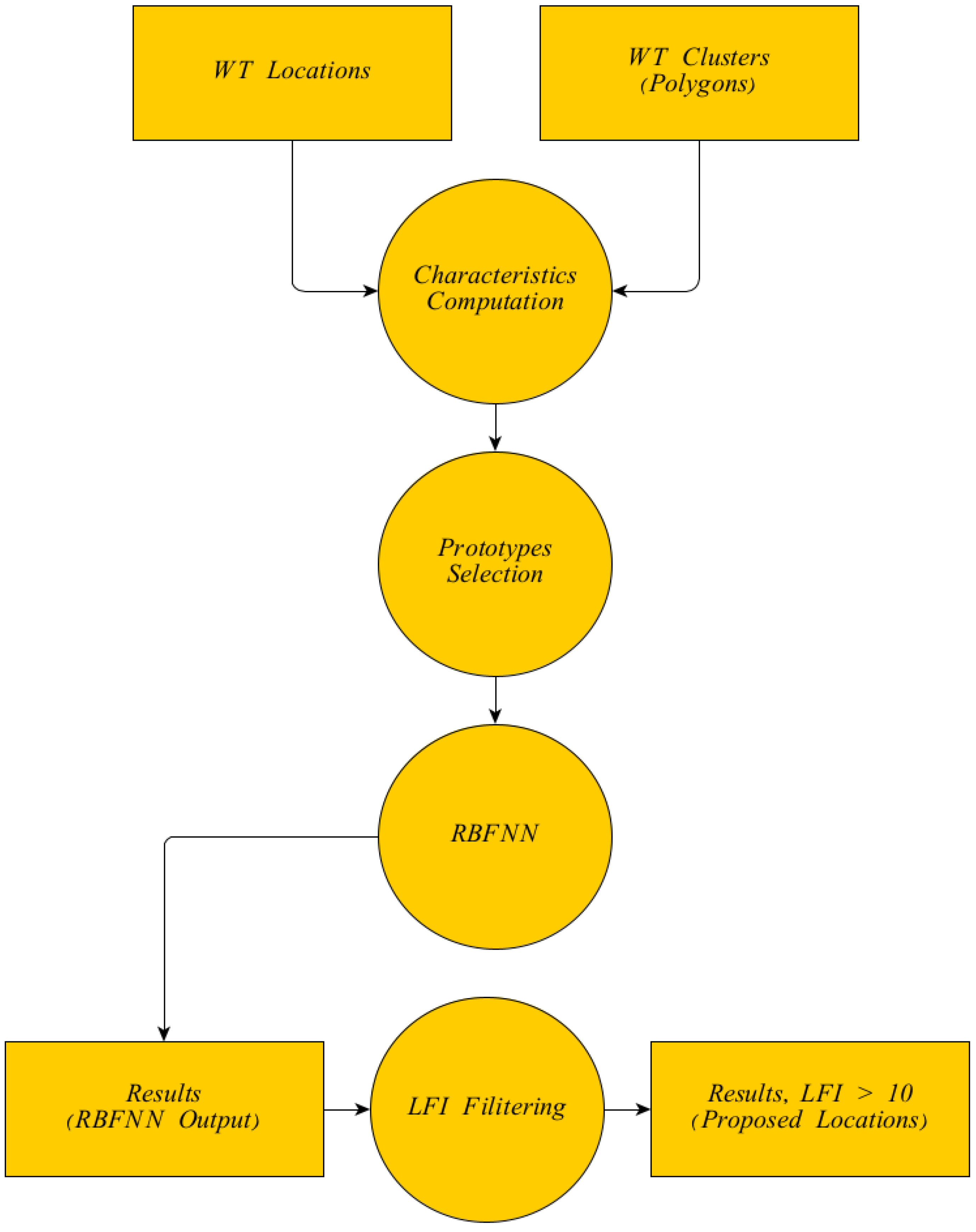
Consequently, the prototypes that correspond to each neuron of the neural network’s RBF layer were determined. The selection of the prototypes was carried out randomly by choosing one point of WT from each of the 158 polygons. Therefore, 158 prototypes were selected, one from each polygon. A map that presents the locations of the prototypes along with the corresponding polygon can be seen in Figure 9 and a sample of their values is presented in

Table 7. A sample of the prototype vectors.

#	C1	C2	C3	C4	C5	C6	C7	C8	C9
1	−1.147	−0.256	2.566	−0.507	−0.815	−0.627	1.027	−0.528	−0.547
2	−1.233	−0.6	−0.56	−0.28	−0.758	−0.497	0.483	−0.368	−0.545
3	−1.205	−0.68	0.596	−0.429	−0.056	−0.1	−1.163	−0.368	0.143
4	−0.206	−0.557	0.494	−0.186	0.143	−0.721	−0.95	−0.112	−0.544
⋮	⋮
156	2.081	−0.366	−0.515	−0.533	−0.947	0.755	−1.283	1.073	2.487
157	−0.945	−0.454	2.704	−0.463	0.194	−0.323	0.406	0.753	−0.546
158	−1.068	−0.485	−0.208	−0.398	−0.386	0.488	−0.756	0.592	−0.547

. As a result, the RBF layer of the proposed RBFNN consists of 158 neurons.

In the next stage of the proposed methodology, multiple structures of NNs were tested and the most efficient one was chosen. In order to train and test the NNs, a set of 10,904 vectors, corresponding to the WTs that were not characterized as outliers, was randomly separated into 7632 (70%) training vectors and 3272 (30%) testing vectors. A sample of the input data (training and testing vectors) is presented in

Table 8. A sample of the input vectors.

	Input									Output
#	C1	C2	C3	C4	C5	C6	C7	C8	C9	#1	#2	#3	#4
1	−1.194	−0.358	2.502	−0.508	−0.336	−0.641	0.996	−0.527	−0.546	0	1	0	0
2	−0.097	−0.43	−0.385	−0.526	2.283	0.424	0.14	−0.207	−0.546	1	0	0	0
3	−0.101	−0.435	−0.206	−0.513	2.227	0.438	0.296	−0.047	−0.545	1	0	0	0
4	−0.103	−0.4	−0.25	−0.487	1.48	0.462	−0.048	0.112	−0.545	1	0	0	0
⋮	⋮									⋮
10902	0.441	−0.334	2.137	−0.184	0.17	−0.368	0.463	1.712	−0.543	1	0	0	0
10903	2.098	0.23	−0.412	−0.39	−0.381	1.246	−0.536	2.192	−0.547	0	0	0	1
10904	0.338	−0.661	0.827	−0.575	1.257	−0.523	0.025	−0.527	2.007	1	0	0	0

. An RBFNN with no extra hidden layer and RBFNNs with one extra hidden layer, consisting of a number of neurons that range from 1 to 200, were built and implemented using the “MLPClassifier” class of the “schikit-learn” library of PYTHON. The validation score for the set of testing vectors for each NN was computed and the results can be seen in Figure 10a. The validation score of the RBFNN with no extra hidden layer was about 0.7 and its value increases for the RBFNNs with one extra hidden layer as the number of neurons raises. A stabilization of the validation score, in values greater than 0.95, can be seen in RBFNNs with 70 neurons and more in the extra hidden layer.

As a result, a RBFNN with 100 neurons in an extra hidden layer was chosen to be trained. In order to evaluate if there was an overfitting problem, the validation score and the current loss were computed for each iteration. For this purpose, the parameter “early_stopping” of the class “MLPClassifier” was set to “True” and 10% of the training data were automatically used for computing the validation score at the end of each iteration. The values of the loss and the validation score for each iteration are presented in Figure 10b. The validation score keeps improving throughout all the iterations and no decrement can be seen. Similarly, the current loss lowers its values throughout the training. Therefore, it can be assumed that no overfitting occurs.

Proposed Locations

At the last stage of the proposed methodology, 10,000 points, similarly distributed in the land of Greece, were randomly selected. Points that are within protected areas and points that are within polygons $\mathcal{C}\left(\mathcal{WT}\right)$ were excluded from the potential locations. As a result, 7934 points remained as locations that are available for WF investment and were tested for their compatibility. In order to input the potential locations into the RBFNN, the characteristics of Table 1 were computed and the values were normalized using the z-scores that were extracted from the corresponding values of the training set.

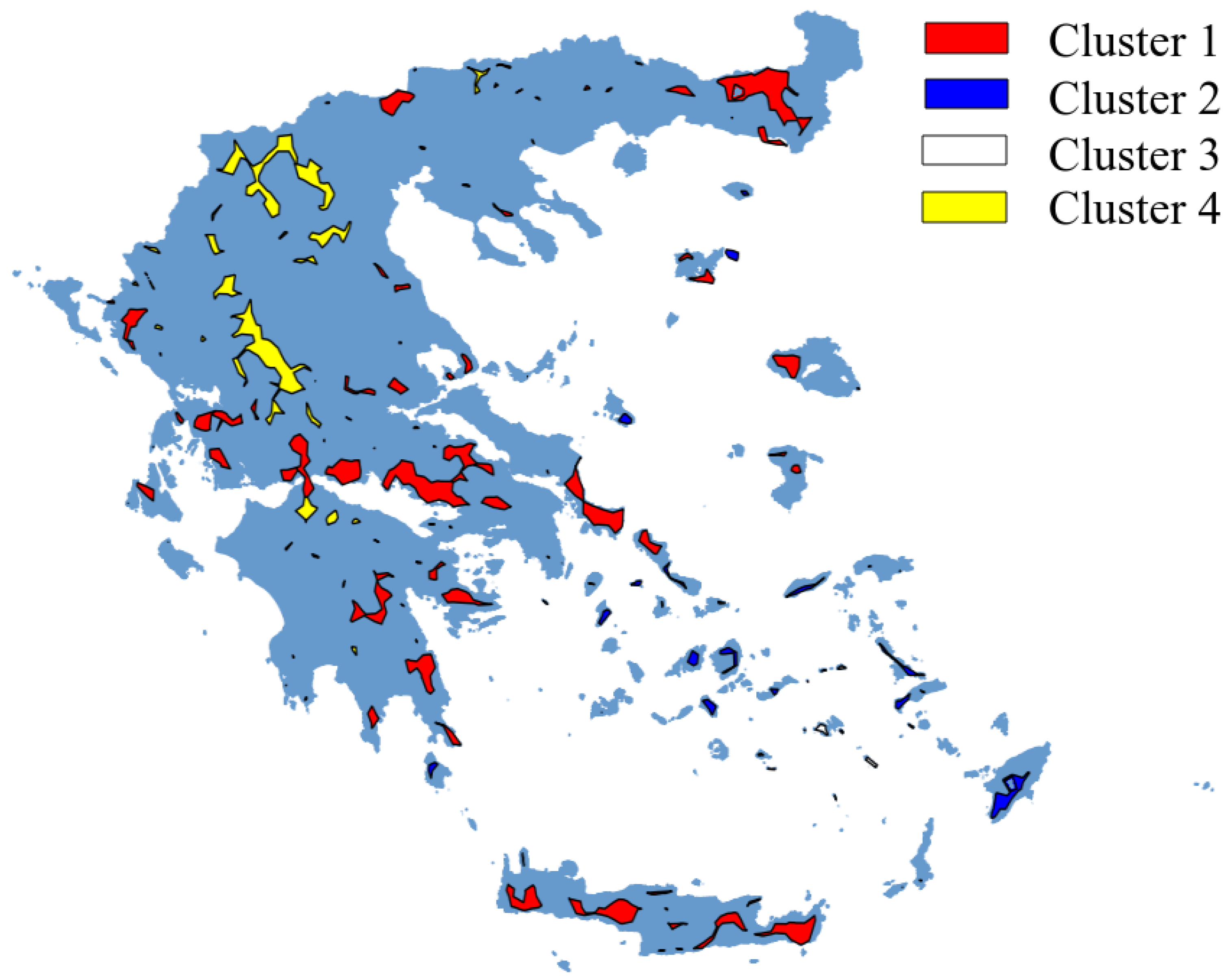
The locations that were evaluated as optimal for WF development by the RBFNN are presented in Figure 11. A total of 1396 points were classified to cluster #1 and are presented in red, 151 were classified to cluster #2 and are presented in blue, 3 were classified to cluster #3 and are presented in black and 133 were classified to cluster #4 and are presented in yellow. Consequently, the points that are within areas with LFI less than 10 were excluded from the proposed locations as they are not preferable for WF development. Finally, 716 locations from cluster #1 and 88 locations from cluster #2 were exported by the RBFNN and, simultaneously, they are within areas with LFI greater or equal than 10; these points are presented in Figure 12. The number of the locations for each case can be seen in

Table 9. The number of proposed locations per cluster, separated by LFI preferable and not preferable values.

Cluster	Proposed	LFI < 10 (Not Preferable)	LFI ≥ 10 (Preferable)
#1	1396	680	716
#2	151	63	88
#3	3	3	0
#4	133	133	0
Total	1683	879	804

.

4. Discussion

Public acceptance of RES is questionable. Although many understand that energy production from renewable sources can be a viable energy production solution, at the same time, they request that this type of investment be installed as far away from their communities as possible [90].

While the transition to renewable-energy-based systems is generally perceived as positive, the local implementation of projects and the extension of the grid are often not accepted by the public [91]. For this reason, social research has placed much of its focus on understanding the social acceptance of renewable energy technologies [92].

So far, researchers have mostly focused on explaining phenomena related to the non-acceptance or rejection of renewables, without, however, reaching a deeper analysis of the different aspects of acceptance and support [93]. Social acceptance, described as the public’s active or passive approval of a certain policy [91], is one of the most prominent barriers to achieve renewable energy targets. At the same time, there is the risk of neglecting the active participation of the public in the transition towards a renewable-energy-based system. In addition, the existing studies examine public acceptance as the (static) position of a certain (or more) factor(s) in relation to a specific RES project in one specific country, thus adopting an approach that is based on cases.

Despite the significant advantages of renewable energy sources, the wider uncertainty that surrounds the local effects of renewable energy plants has a negative effect on social acceptance. There can be a distinction between “general social acceptance” and “local social acceptance”, with the first referring to social acceptance on a wider level that can also be characterized as socio-political acceptance. The second type of acceptance refers to the community level and is related to the siting of renewable energy projects.

In many countries of the European Union, the percentage of public acceptance of renewable energy is high. That being said, it has also been observed that, when the local community is affected directly by the construction of a renewable plant, the lack of local acceptance increases, which may even result in the cancellation of entire projects. There is an increasing number of case studies that focus on these phenomena. In other cases, a diverse range of relational factors, which contribute to the formation of social acceptance, are fundamental steps towards acceptance. Such factors were studied by Segreto et al. [94], Wüstenhagen et al. [95] and Caporale and De Lucia [96] and involve trust in authorities, information dissemination, public participation and economic benefits.

On the other side of the coin, research has pointed to the negative effects of renewable projects on protected environmental areas, avian habitats, vulnerable ecosystems, but also on the attractiveness and the recreational value of natural landscapes [97]. Such findings have raised concerns about the spatial planning and environmental and social effects of large-scale renewable projects. In this context, much research focuses on the optimization of wind parks and the visual aspects of wind turbines as well as on their impacts on ecosystems and nature preservation [98]. That being said, this kind of approach should not be confused with the creation of broad base scenarios and the inclusion of nature preservation as a criterion. Wind energy scenarios take into account only economic and technical factors [99].

Moreover, the noise that is emitted by a wind turbine is a factor that negatively affects social acceptance. The acoustic characterization of noise in environments close to WTs was studied thoroughly by Ciaburro et al. [100]. The problem described has been even more perceivable in recent years due to new technologies of WTs where taller and more powerful towers are suggested. As a result, the landscape fragmentation index is an important factor in WT allocation, due to the fact that areas with high LFI values can support the installation of higher WTs that produce more noise. Additionally, the model proposed in the current study has been designed in a way that can accept new variables when available, thus it can be configured to be trained in a second stage with extra WT characteristics, such as their height or the diameter of their rotor blade.

In conclusion, it may be argued that the European Union has prepared plans that involve the deployment of renewable energy at a higher level. As social acceptance is a critical barrier to RES deployment, governments ought to consider local acceptance and create a framework that will increase the possibility of social acceptance, thereby reducing opposition networks that often inhibit RES development. Trust in major factors continues to be a social acceptance lever and it has been observed that the public needs to trust local authorities and investors in order to accept RES projects. This trust should be built through a transparent process and should extend to the entire chain from project planning to development and implementation. Moreover, the provision of quality information and public participation in the planning processes consists of an institutional factor of social acceptance. Information provided to the public should be characterized by high technical quality and include data related to the economic and environmental effects.

Therefore, extensive studies must be carried out for the proposal of installation locations which are acceptable to the general public.

Additionally, most of the studies which deal with the problem of RES installation use a combination of criteria. Depending on the researcher’s point of view, these criteria may include legislation, spatial characteristics (topography, elevation aspect, etc.), infrastructure characteristics (road network, energy transfer network), meteorological conditions (wind speed, wind direction, rain data, etc.), economic criteria (installation costs, maintenance costs) and, finally, WT types, energy production capabilities and conversion efficiency.

After evaluating the impact of each criterion on problem-solving, they are usually combined using multicriteria decision analysis techniques and, subsequently, the results are presented in a geographical information system. The results can be further evaluated and refined by applying ranking methods like TOPSIS, which can create a ranking of the proposed installation locations.

Although these approaches are sound, they include a number of drawbacks:

• The number of criteria used;
• The evaluation of the criteria and their weight coefficients;
• The addition or exclusion of criteria requires the entire methodology to be reapplied.

Additionally, almost all of the studies which propose installation locations do not take into account (and are optimized for) the land fragmentation index (LFI) of the areas under investigation or create exclusion zones based on protected areas (as these are defined by the national and European legislations).

Hence, there is a need for developing a new unbiased methodology not only capable of reading and internally incorporating the criteria used in all previous studies but, at the same time, of understanding the social acceptance level, which is a key factor when it comes to the installation of WTs.

This type of approach can be based on the usage of Machine Learning in order to evaluate current installations on the grounds that, if they are already installed, then the following parameters must be met:

• The investment is acceptable to the locals;
• The investment is compatible with the legislation;
• The investment meets the other installation requirements (criteria).

The algorithm we have developed has as input the characteristics from all WTs across Greece, which are spatially expressed in the form of installation locations and, based on these, they are able to estimate new possible investment locations with two major improvements. The first improvement is that protected areas (nature sites, etc.) are automatically excluded from future locations and the second is that the LFI is taken into account.

We believe that these two improvements, in combination with the unbiased understanding of the previously installation locations, will enhance the social acceptance of WT. The ML algorithm will propose new investment positions which will not only be outside protected areas (a constant request from the communities, which, however, is not a requirement of the existing legislation) but it will also propose their installation in the areas that are already the most fragmented. These heavily fragmented areas can include the sides of motorways, railway tracks, energy transfer networks, etc.

Consequently, the k-means algorithm was applied to the set of polygons defining the areas of the previously installed WTs in order to comprehend their characteristics. It was found that these areas could be divided into four clusters. Clustering can be an important tool for decision makers who can draw important conclusions about the characteristics of the areas where WTs are installed. It is simple to identify the impacts, both positive and negative, that the operation of WTs has on the wider area. This information can be used by those in charge when selecting new locations for RES installation.

Cluster #1 contains the most areas and the most WTs compared to the other three clusters. It is mostly found on the Greek mainland and the island of Crete and it consists of semi-mountainous areas. It can be noticed that the areas of this cluster are both reasonably close to residential areas and to airports. Therefore, there is an increased risk of negative reactions from the residents of the wider area due to the visual impact and noise caused by the WTs. In addition, it is possible that the WTs of this cluster affect the operation of the airports. On the contrary, these areas are very close to the road network and at a relatively low altitude, which significantly reduces installation costs.

Cluster #4 is located in areas that are relatively high in altitude, mainly on the Greek mainland. Moreover, the areas of this cluster are closer to protected areas compared to the other clusters. Given that the majority of the protected areas are found in mountainous regions, this was to be expected. Finally, they are quite far from the country’s airports, so there is no risk of disturbance when the planes approach them.

Cluster #2 consists of island regions, mainly in the Dodecanese and the Cyclades. Therefore, they are only a very short distance from the Greek coastline and are located at a relatively low altitude. Their long distance from the road network is one of their drawbacks, but it is offset by the high wind potential that is seen in these areas.

Cluster #3 consists of a very small number of WTs in areas located on small islands in the Aegean. These wind turbines are located very close to the coastline and at almost zero altitude. Compared to the other clusters, their distance from the road network is the longest; however, the wind potentials of these areas have the highest values.

In the next step of the methodology, an RBFNN was trained in order to evaluate new locations for WF investment. The results of the RBFNN-based algorithm’s application are displayed in Figure 11. However, these results obviously need to be improved mainly because the algorithm proposes as potential installation locations areas which are close to tourist destinations, close to residential areas or inside protected areas. The suggested locations are significantly improved when the results and findings are combined with the LFI and the exclusion of protected areas (Figure 12). This improvement focuses on the social acceptance of the proposed locations (by excluding protected areas) as well as the installation on already highly fragmented areas. For example, on the island of Thassos, the initial results included almost the entire island. However, the improved results include only a section of the east part of the island. Similar results were obtained for the island of Samothraki, the Pindos mountain range, etc. In all of the cases, the initial results were heavily influenced by the legislation, spatial characteristics and meteorological conditions. The inclusion of factors such as the exclusion of protected areas and the LFI, which are also factors that drive social acceptance, resulted in locations which we believe can be used for installation without negatively impacting local communities and the environment.

Following extensive research into related studies that were focused on the area of Greece, it was found that there is no study that has implemented its proposed methodology in the entire Greek territory; instead, they are limited in specific areas of Greece and they develop their methodology only taking into account the particular characteristics of the corresponding region.

Konstantinos et al. [17] developed a case study in the region of Eastern Macedonia and Thrace, and, more specifically, in the Drama prefecture using MCDM and AHP. The proposed locations extracted by their model are similar to the locations proposed in the current study, especially the locations inside the red frames that can be seen in Figure 13, where the locations of the two studies coincide. Nevertheless, the locations that were proposed in the Drama prefecture are all in areas with low LFI values; they were thus excluded by the proposed locations of our study in the last stage of the procedure.

Additionally, the locations proposed for WF development by Latinopoulos and Kechagia [39] in the regional unit of Kozani, which is part of the prefecture of Western Macedonia in Greece, coincide with the locations proposed by our study in the current area (Figure 14). Even though Latinopoulos and Kechagia [39] include these locations in their proposed area, they evaluate them with low and medium suitability. Similarly, these locations have been excluded from the areas proposed by our study, due to the fact that they are within areas with LFI values less than 10.

Obviously, the results from the aforementioned studies are similar to the initial results presented here. However, by applying the LFI, we enhance these results by proposing the installation of WFs on already highly fragmented areas.

5. Conclusions

Although RES, and, in particular, WTs, are considered to be a liable and sustainable method for energy production, there are many cases in which local communities present negative reactions. The popular point of view—“not in my back yard”—is creating tidal effects wherever WF investment is considered. Although many of the previous studies which deal with the problem of installation location optimization have provided acceptable results, almost all of them fail to incorporate the LFI and the exclusion of protected areas. Both of these parameters are what differentiates our approach from previous approaches. We build on previous knowledge (in the form of the produced results) by applying the RBFNN algorithm and, on the produced results, we incorporate the aforementioned parameters.

References

1. Bórawski, P.; Bełdycka-Bórawska, A.; Szymańska, E.J.; Jankowski, K.J.; Dubis, B.; Dunn, J.W. Development of renewable energy sources market and biofuels in The European Union. J. Clean. Prod. 2019, 228, 467–484. [Google Scholar] [CrossRef]
2. EurObserv’ER. Photovoltaic Barometer 2022. 2022. Available online: https://www.eurobserv-er.org/photovoltaic-barometer-2022/ (accessed on 24 April 2023).
3. EurObserv’ER. Wind Energy Barometer 2022. 2022. Available online: https://www.eurobserv-er.org/wind-energy-barometer-2022/ (accessed on 24 April 2023).
4. Eurostat. Renewable Energy Statistics. 2022. Available online: https://www.irena.org/publications/2022/Jul/Renewable-Energy-Statistics-2022 (accessed on 24 April 2023).
5. Megura, M.; Gunderson, R. Better poison is the cure? Critically examining fossil fuel companies, climate change framing, and corporate sustainability reports. Energy Res. Soc. Sci. 2022, 85, 102388. [Google Scholar] [CrossRef]
6. Chiari, L.; Zecca, A. Constraints of fossil fuels depletion on global warming projections. Energy Policy 2011, 39, 5026–5034. [Google Scholar] [CrossRef]
7. Braungardt, S.; van den Bergh, J.; Dunlop, T. Fossil fuel divestment and climate change: Reviewing contested arguments. Energy Res. Soc. Sci. 2019, 50, 191–200. [Google Scholar] [CrossRef]
8. Zecca, A.; Chiari, L. Fossil-fuel constraints on global warming. Energy Policy 2010, 38, 1–3. [Google Scholar] [CrossRef]
9. Tutak, M.; Brodny, J. Renewable energy consumption in economic sectors in the EU-27. The impact on economics, environment and conventional energy sources. A 20-year perspective. J. Clean. Prod. 2022, 345, 131076. [Google Scholar] [CrossRef]
10. Poudyal, R.; Loskot, P.; Nepal, R.; Parajuli, R.; Khadka, S.K. Mitigating the current energy crisis in Nepal with renewable energy sources. Renew. Sustain. Energy Rev. 2019, 116, 109388. [Google Scholar] [CrossRef]
11. Pietrosemoli, L.; Rodríguez-Monroy, C. The Venezuelan energy crisis: Renewable energies in the transition towards sustainability. Renew. Sustain. Energy Rev. 2019, 105, 415–426. [Google Scholar] [CrossRef]
12. Meza, C.G.; Amado, N.B.; Sauer, I.L. Transforming the Nicaraguan energy mix towards 100% renewable. Energy Procedia 2017, 138, 494–499. [Google Scholar] [CrossRef]
13. De Rosa, M.; Gainsford, K.; Pallonetto, F.; Finn, D.P. Diversification, concentration and renewability of the energy supply in the European Union. Energy 2022, 253, 124097. [Google Scholar] [CrossRef]
14. Laimon, M.; Mai, T.; Goh, S.; Yusaf, T. System dynamics modelling to assess the impact of renewable energy systems and energy efficiency on the performance of the energy sector. Renew. Energy 2022, 193, 1041–1048. [Google Scholar] [CrossRef]
15. Li, W.; Ji, Z.; Dong, F. Global renewable energy power generation efficiency evaluation and influencing factors analysis. Sustain. Prod. Consum. 2022, 33, 438–453. [Google Scholar] [CrossRef]
16. What Is Carbon Neutrality and How Can It Be Achieved by 2050?|News|European Parliament. 2019. Available online: https://www.europarl.europa.eu/news/en/headlines/society/20190926STO62270/what-is-carbon-neutrality-and-how-can-it-be-achieved-by-2050 (accessed on 12 April 2023).
17. Konstantinos, I.; Georgios, T.; Garyfalos, A. A Decision Support System methodology for selecting wind farm installation locations using AHP and TOPSIS: Case study in Eastern Macedonia and Thrace region, Greece. Energy Policy 2019, 132, 232–246. [Google Scholar] [CrossRef]
18. Gorsevski, P.V.; Cathcart, S.C.; Mirzaei, G.; Jamali, M.M.; Ye, X.; Gomezdelcampo, E. A group-based spatial decision support system for wind farm site selection in Northwest Ohio. Energy Policy 2013, 55, 374–385. [Google Scholar] [CrossRef]
19. Salvador, C.B.; Arzaghi, E.; Yazdi, M.; Jahromi, H.A.F.; Abbassi, R. A multi-criteria decision-making framework for site selection of offshore wind farms in Australia. Ocean Coast. Manag. 2022, 224, 106196. [Google Scholar] [CrossRef]
20. Tegou, L.I.; Polatidis, H.; Haralambopoulos, D.A. Environmental management framework for wind farm siting: Methodology and case study. J. Environ. Manag. 2010, 91, 2134–2147. [Google Scholar] [CrossRef]
21. Saraswat, S.K.; Digalwar, A.K.; Yadav, S.S.; Kumar, G. MCDM and GIS based modelling technique for assessment of solar and wind farm locations in India. Renew. Energy 2021, 169, 865–884. [Google Scholar] [CrossRef]
22. Bennui, A.; Rattanamanee, P.; Puetpaiboon, U.; Phukpattaranont, P.; Chetpattananondh, K. Site selection for large wind turbine using GIS. In Proceedings of the PSU-UNS International Conference on Engineering and Environment, Phuket, Thailand, 10–11 May 2007; pp. 561–566. [Google Scholar]
23. Xu, Y.; Li, Y.; Zheng, L.; Cui, L.; Li, S.; Li, W.; Cai, Y. Site selection of wind farms using GIS and multi-criteria decision making method in Wafangdian, China. Energy 2020, 207, 118222. [Google Scholar] [CrossRef]
24. Shorabeh, S.N.; Firozjaei, H.K.; Firozjaei, M.K.; Jelokhani-Niaraki, M.; Homaee, M.; Nematollahi, O. The site selection of wind energy power plant using GIS-multi-criteria evaluation from economic perspectives. Renew. Sustain. Energy Rev. 2022, 168, 112778. [Google Scholar] [CrossRef]
25. Al-Yahyai, S.; Charabi, Y.; Gastli, A.; Al-Badi, A. Wind farm land suitability indexing using multi-criteria analysis. Renew. Energy 2012, 44, 80–87. [Google Scholar] [CrossRef]
26. Höfer, T.; Sunak, Y.; Siddique, H.; Madlener, R. Wind farm siting using a spatial Analytic Hierarchy Process approach: A case study of the Städteregion Aachen. Appl. Energy 2016, 163, 222–243. [Google Scholar] [CrossRef]
27. Gigović, L.; Pamučar, D.; Božanić, D.; Ljubojević, S. Application of the GIS-DANP-MABAC multi-criteria model for selecting the location of wind farms: A case study of Vojvodina, Serbia. Renew. Energy 2017, 103, 501–521. [Google Scholar] [CrossRef]
28. Georgiou, A.; Polatidis, H.; Haralambopoulos, D. Wind Energy Resource Assessment and Development: Decision Analysis for Site Evaluation and Application. In Energy Sources, Part A: Recovery, Utilization, and Environmental Effects; Taylor & Francis: Abingdon, UK, 2012; Volume 34, pp. 1759–1767. [Google Scholar] [CrossRef]
29. Tercan, E. Land suitability assessment for wind farms through best-worst method and GIS in Balıkesir province of Turkey. Sustain. Energy Technol. Assess. 2021, 47, 101491. [Google Scholar] [CrossRef]
30. Atici, K.B.; Simsek, A.B.; Ulucan, A.; Tosun, M.U. A GIS-based Multiple Criteria Decision Analysis approach for wind power plant site selection. Util. Policy 2015, 37, 86–96. [Google Scholar] [CrossRef]
31. Ayodele, T.R.; Ogunjuyigbe, A.S.O.; Odigie, O.; Munda, J.L. A multi-criteria GIS based model for wind farm site selection using interval type-2 fuzzy analytic hierarchy process: The case study of Nigeria. Appl. Energy 2018, 228, 1853–1869. [Google Scholar] [CrossRef]
32. Ali, S.; Taweekun, J.; Techato, K.; Waewsak, J.; Gyawali, S. GIS based site suitability assessment for wind and solar farms in Songkhla, Thailand. Renew. Energy 2019, 132, 1360–1372. [Google Scholar] [CrossRef]
33. Sliz-Szkliniarz, B.; Vogt, J. GIS-based approach for the evaluation of wind energy potential: A case study for the Kujawsko–Pomorskie Voivodeship. Renew. Sustain. Energy Rev. 2011, 15, 1696–1707. [Google Scholar] [CrossRef]
34. Sánchez-Lozano, J.M.; García-Cascales, M.S.; Lamata, M.T. Identification and selection of potential sites for onshore wind farms development in Region of Murcia, Spain. Energy 2014, 73, 311–324. [Google Scholar] [CrossRef]
35. Azizi, A.; Malekmohammadi, B.; Jafari, H.R.; Nasiri, H.; Amini Parsa, V. Land suitability assessment for wind power plant site selection using ANP-DEMATEL in a GIS environment: Case study of Ardabil province, Iran. Environ. Monit. Assess. 2014, 186, 6695–6709. [Google Scholar] [CrossRef]
36. Noorollahi, Y.; Yousefi, H.; Mohammadi, M. Multi-criteria decision support system for wind farm site selection using GIS. Sustain. Energy Technol. Assess. 2016, 13, 38–50. [Google Scholar] [CrossRef]
37. Amjad, F.; Agyekum, E.B.; Shah, L.A.; Abbas, A. Site location and allocation decision for onshore wind farms, using spatial multi-criteria analysis and density-based clustering. A techno-economic-environmental assessment, Ghana. Sustain. Energy Technol. Assess. 2021, 47, 101503. [Google Scholar] [CrossRef]
38. Sunak, Y.; Höfer, T.; Siddique, H.; Madlener, R.; De Doncker, R.W. A GIS-Based Decision Support System for the Optimal Siting of Wind Farm Projects; Universitätsbibliothek der RWTH Aachen: Aachen, Germany, 2015. [Google Scholar]
39. Latinopoulos, D.; Kechagia, K. A GIS-based multi-criteria evaluation for wind farm site selection. A regional scale application in Greece. Renew. Energy 2015, 78, 550–560. [Google Scholar] [CrossRef]
40. Fan, B. A hybrid spatial data clustering method for site selection: The data driven approach of GIS mining. Expert Syst. Appl. 2009, 36, 3923–3936. [Google Scholar] [CrossRef]
41. Shaheen, M.; Khan, M.Z. A method of data mining for selection of site for wind turbines. Renew. Sustain. Energy Rev. 2016, 55, 1225–1233. [Google Scholar] [CrossRef]
42. Baban, S.M.J.; Parry, T. Developing and applying a GIS-assisted approach to locating wind farms in the UK. Renew. Energy 2001, 24, 59–71. [Google Scholar] [CrossRef]
43. Asadi, M.; Pourhossein, K.; Mohammadi-Ivatloo, B. GIS-assisted modeling of wind farm site selection based on support vector regression. J. Clean. Prod. 2023, 390, 135993. [Google Scholar] [CrossRef]
44. Asadi, M.; Pourhossein, K. Locating Renewable Energy Generators Using K-Nearest Neighbors (KNN) Algorithm. In Proceedings of the 2019 Iranian Conference on Renewable Energy & Distributed Generation (ICREDG), Tehran, Iran, 11–12 June 2019; pp. 1–6. [Google Scholar] [CrossRef]
45. Pennell, W.T.; Barchet, W.R.; Elliott, D.L.; Wendell, L.L.; Hiester, T.R. Meteorological aspects of wind energy: Assessing the resource and selecting the sites. J. Wind Eng. Ind. Aerodyn. 1980, 5, 223–246. [Google Scholar] [CrossRef]
46. Janke, J.R. Multicriteria GIS modeling of wind and solar farms in Colorado. Renew. Energy 2010, 35, 2228–2234. [Google Scholar] [CrossRef]
47. Ayodele, T.R.; Ogunjuyigbe, A.S.O.; Odigie, O.; Jimoh, A.A. On the most suitable sites for wind farm development in Nigeria. Data Brief 2018, 19, 29–41. [Google Scholar] [CrossRef]
48. Asadi, M.; Pourhossein, K. Wind farm site selection considering turbulence intensity. Energy 2021, 236, 121480. [Google Scholar] [CrossRef]
49. Rodman, L.C.; Meentemeyer, R.K. A geographic analysis of wind turbine placement in Northern California. Energy Policy 2006, 34, 2137–2149. [Google Scholar] [CrossRef]
50. Fetanat, A.; Khorasaninejad, E. A novel hybrid MCDM approach for offshore wind farm site selection: A case study of Iran. Ocean Coast. Manag. 2015, 109, 17–28. [Google Scholar] [CrossRef]
51. Watson, J.J.W.; Hudson, M.D. Regional Scale wind farm and solar farm suitability assessment using GIS-assisted multi-criteria evaluation. Landsc. Urban Plan. 2015, 138, 20–31. [Google Scholar] [CrossRef]
52. Lalas, D.P.; Tselepidaki, H.; Theoharatos, G. An analysis of wind power potential in Greece. Sol. Energy 1983, 30, 497–505. [Google Scholar] [CrossRef]
53. Katsoulis, B.D.; Metaxas, D.A. The wind energy potential of western greece. Sol. Energy 1992, 49, 463–476. [Google Scholar] [CrossRef]
54. Voivontas, D.; Assimacopoulos, D.; Mourelatos, A.; Corominas, J. Evaluation of Renewable Energy potential using a GIS decision support system. Renew. Energy 1998, 13, 333–344. [Google Scholar] [CrossRef]
55. Oikonomou, E.K.; Kilias, V.; Goumas, A.; Rigopoulos, A.; Karakatsani, E.; Damasiotis, M.; Papastefanakis, D.; Marini, N. Renewable energy sources (RES) projects and their barriers on a regional scale: The case study of wind parks in the Dodecanese islands, Greece. Energy Policy 2009, 37, 4874–4883. [Google Scholar] [CrossRef]
56. RAE GeoPortal. Regulatory Authority for Energy. 2022. Available online: https://geo.rae.gr/ (accessed on 18 December 2022).
57. Datasets—geodata.gov.gr. 2022. Available online: https://geodata.gov.gr/en/dataset (accessed on 21 July 2022).
58. Global Wind Atlas. 2022. Available online: https://globalwindatlas.info/en (accessed on 20 August 2022).
59. European Environment Agency. Europe Coastline Shapefile. Available online: https://www.eea.europa.eu/data-and-maps/data/eea-coastline-for-analysis-1/gis-data/europe-coastline-shapefile (accessed on 25 August 2022).
60. Faris, H.; Aljarah, I.; Mirjalili, S. Evolving Radial Basis Function Networks Using tMoth—Flame Optimizer; Academic Press: Cambridge, MA, USA, 2017. [Google Scholar]
61. Ekblad, U. Radial Basis Function Networks (RBFN). Ph.D. Thesis, Tryck—Universitetsservice USAB, Stockholm, Sweden, 2002. [Google Scholar]
62. Dubuisson, B. Neural Networks, General Principles. In Encyclopedia of Vibration; Braun, S., Ed.; Elsevier: Oxford, UK, 2001; pp. 869–877. [Google Scholar] [CrossRef]
63. Vt, S.E.; Shin, Y.C. Radial basis function neural network for approximation and estimation of nonlinear stochastic dynamic systems. IEEE Trans. Neural Netw. 1994, 5, 594–603. [Google Scholar] [CrossRef]
64. Lee, C.C.; Chung, P.C.; Tsai, J.R.; Chang, C.I. Robust radial basis function neural networks. IEEE Trans. Syst. Man Cybern. Part B Cybern. 1999, 29, 674–685. [Google Scholar] [CrossRef]
65. Hwang, Y.S.; Bang, S.Y. An Efficient Method to Construct a Radial Basis Function Neural Network Classifier. Neural Netw. 1997, 10, 1495–1503. [Google Scholar] [CrossRef]
66. Zhao, Y.; Pei, J.; Chen, H. Multi-layer radial basis function neural network based on multi-scale kernel learning. Appl. Soft Comput. 2019, 82, 105541. [Google Scholar] [CrossRef]
67. Jiang, Q.; Zhu, L.; Shu, C.; Sekar, V. An efficient multilayer RBF neural network and its application to regression problems. Neural Comput. Appl. 2022, 34, 4133–4150. [Google Scholar] [CrossRef]
68. Wen, H.; Yan, T.; Liu, Z.; Chen, D. Integrated neural network model with pre-RBF kernels. Sci. Prog. 2021, 104, 00368504211026111. [Google Scholar] [CrossRef] [PubMed]
69. Kuncheva, L.I. Initializing of an RBF network by a genetic algorithm. Neurocomputing 1997, 14, 273–288. [Google Scholar] [CrossRef]
70. Simon, D. Training radial basis neural networks with the extended Kalman filter. Neurocomputing 2002, 48, 455–475. [Google Scholar] [CrossRef]
71. Gonzalez, J.; Rojas, H.; Ortega, J.; Prieto, A. A new clustering technique for function approximation. IEEE Trans. Neural Netw. 2002, 13, 132–142. [Google Scholar] [CrossRef] [PubMed]
72. Staiano, A.; Tagliaferri, R.; Pedrycz, W. Improving RBF networks performance in regression tasks by means of a supervised fuzzy clustering. Neurocomputing 2006, 69, 1570–1581. [Google Scholar] [CrossRef]
73. Ferreira Cruz, D.P.; Dourado Maia, R.; da Silva, L.A.; de Castro, L.N. BeeRBF: A bee-inspired data clustering approach to design RBF neural network classifiers. Neurocomputing 2016, 172, 427–437. [Google Scholar] [CrossRef]
74. Barzilai, J. Chapter 15—On neural-network training algorithms. In Human-Machine Shared Contexts; Lawless, W.F., Mittu, R., Sofge, D.A., Eds.; Academic Press: Cambridge, MA, USA, 2020; pp. 307–313. [Google Scholar] [CrossRef]
75. Khare, V.; Khare, C.; Nema, S.; Baredar, P. (Eds.) Chapter 2—Data visualization and descriptive statistics of solar energy system. In Decision Science and Operations Management of Solar Energy Systems; Academic Press: Cambridge, MA, USA, 2023; pp. 33–75. [Google Scholar] [CrossRef]
76. Ball, G.H.; Hall, D.J. A clustering technique for summarizing multivariate data. Behav. Sci. 1967, 12, 153–155. [Google Scholar] [CrossRef]
77. Jain, A.K. Data clustering: 50 years beyond K-means. Pattern Recognit. Lett. 2010, 31, 651–666. [Google Scholar] [CrossRef]
78. Birsan, T.; Tiba, D. One Hundred Years Since the Introduction of the Set Distance by Dimitrie Pompeiu. In Proceedings of the System Modeling and Optimization—22nd IFIP TC7 Conference, Turin, Italy, 18–22 July 2005; Ceragioli, F., Dontchev, A., Futura, H., Marti, K., Pandolfi, L., Eds.; IFIP International Federation for Information Processing: Boston, MA, USA, 2006; pp. 35–39. [Google Scholar] [CrossRef]
79. Xenitidis, K.; Ioannou, K.; Tsantopoulos, G. An innovative methodology for the determination of wind farms installation location characteristics using GIS and Delaunay Triangulation. Energy Sustain. Dev. 2023, 75, 25–39. [Google Scholar] [CrossRef]
80. Fukushima, K. Visual Feature Extraction by a Multilayered Network of Analog Threshold Elements. IEEE Trans. Syst. Sci. Cybern. 1969, 5, 322–333. [Google Scholar] [CrossRef]
81. Scikit-Learn. Machine Learning in Python—Scikit-Learn 1.3.1 Documentation. Available online: https://scikit-learn.org/stable/index.html (accessed on 12 September 2022).
82. Kingma, D.P.; Ba, J. Adam: A Method for Stochastic Optimization. arXiv 2017, arXiv:1412.6980. [Google Scholar]
83. Salkanović, E. Protecting avian wildlife for wind farm siting: The Screening Tool Proof of Concept. Energy Sustain. Dev. 2023, 74, 66–78. [Google Scholar] [CrossRef]
84. Tsarknias, N.; Gkeka-Serpetsidaki, P.; Tsoutsos, T. Exploring the sustainable siting of floating wind farms in the Cretan coastline. Sustain. Energy Technol. Assess. 2022, 54, 102841. [Google Scholar] [CrossRef]
85. Sotiropoulou, K.F.; Vavatsikos, A.P. Onshore wind farms GIS-Assisted suitability analysis using PROMETHEE II. Energy Policy 2021, 158, 112531. [Google Scholar] [CrossRef]
86. Gkeka-Serpetsidaki, P.; Tsoutsos, T. A methodological framework for optimal siting of offshore wind farms: A case study on the island of Crete. Energy 2022, 239, 122296. [Google Scholar] [CrossRef]
87. Llausàs, A.; Nogué, J. Indicators of landscape fragmentation: The case for combining ecological indices and the perceptive approach. Ecol. Indic. 2012, 15, 85–91. [Google Scholar] [CrossRef]
88. Agency, E.E. Landscape Fragmentation Effective Mesh Density Time Series. Available online: https://www.eea.europa.eu/data-and-maps/data/landscape-fragmentation-effective-mesh-density/landscape-fragmentation-effective-mesh-density (accessed on 4 March 2023).
89. Kati, V.; Kassara, C.; Vrontisi, Z.; Moustakas, A. The biodiversity-wind energy-land use nexus in a global biodiversity hotspot. Sci. Total Environ. 2021, 768, 144471. [Google Scholar] [CrossRef]
90. Tampakis, S.; Tsantopoulos, G.; Arabatzis, G.; Rerras, I. Citizens’ views on various forms of energy and their contribution to the environment. Renew. Sustain. Energy Rev. 2013, 20, 473–482. [Google Scholar] [CrossRef]
91. Bertsch, V.; Hall, M.; Weinhardt, C.; Fichtner, W. Public acceptance and preferences related to renewable energy and grid expansion policy: Empirical insights for Germany. Energy 2016, 114, 465–477. [Google Scholar] [CrossRef]
92. Batel, S. Research on the social acceptance of renewable energy technologies: Past, present and future. Energy Res. Soc. Sci. 2020, 68, 101544. [Google Scholar] [CrossRef]
93. Batel, S.; Castro, P.; Devine-Wright, P.; Howarth, C. Developing a critical agenda to understand pro-environmental actions: Contributions from Social Representations and Social Practices Theories. WIREs Clim. Chang. 2016, 7, 727–745. [Google Scholar] [CrossRef]
94. Segreto, M.; Principe, L.; Desormeaux, A.; Torre, M.; Tomassetti, L.; Tratzi, P.; Paolini, V.; Petracchini, F. Trends in Social Acceptance of Renewable Energy Across Europe—A Literature Review. Int. J. Environ. Res. Public Health 2020, 17, 9161. [Google Scholar] [CrossRef]
95. Wüstenhagen, R.; Wolsink, M.; Bürer, M.J. Social acceptance of renewable energy innovation: An introduction to the concept. Energy Policy 2007, 35, 2683–2691. [Google Scholar] [CrossRef]
96. Caporale, D.; De Lucia, C. Social acceptance of on-shore wind energy in Apulia Region (Southern Italy). Renew. Sustain. Energy Rev. 2015, 52, 1378–1390. [Google Scholar] [CrossRef]
97. Wang, S.; Wang, S. Impacts of wind energy on environment: A review. Renew. Sustain. Energy Rev. 2015, 49, 437–443. [Google Scholar] [CrossRef]
98. Frantál, B.; Bevk, T.; Veelen, B.V.; Hărmănescu, M.; Benediktsson, K. The importance of on-site evaluation for placing renewable energy in the landscape: A case study of the Búrfell wind farm (Iceland). Morav. Geogr. Rep. 2017, 25, 234–247. [Google Scholar] [CrossRef]
99. Gauglitz, P.; Schicketanz, S.; Pape, C. Nature conservation as a driver in wind energy scenarios. Energy Sustain. Soc. 2019, 9, 47. [Google Scholar] [CrossRef]
100. Ciaburro, G.; Iannace, G.; Puyana-Romero, V.; Trematerra, A. Machine Learning-Based Tools for Wind Turbine Acoustic Monitoring. Appl. Sci. 2021, 11, 6488. [Google Scholar] [CrossRef]
Figure 1. The locations of WTs in Greece.
Sustainability 15 16938 g001
Figure 2. The structure of an RBFNN.
Sustainability 15 16938 g002
Figure 3. Methodology diagram.
Sustainability 15 16938 g003
Figure 4. The structure of the proposed RBFNN.
Sustainability 15 16938 g004
Figure 5. The data that are imported to each layer of the RBFNN.
Sustainability 15 16938 g005
Figure 6. The activation functions of the neurons. (a) Gaussian RBF ϕ x = e 0.5 · x 2 . (b) The activation function of the hidden layer f ( x ) = max 0 , x .
Sustainability 15 16938 g006
Figure 7. The map of Landscape Fragmentation Indicator zones in Greece.
Sustainability 15 16938 g007
Figure 8. Histograms and density curves for each characteristic. Separate lines for the whole set of points and for each cluster. (a) Distance from airports. (b) Distance from road network. (c) Distance from protected areas. (d) Wind speed. (e) Elevation. (f) Slope. (g) Distance from coastline. (h) Distance from rivers. (i) Distance from residential areas.
Sustainability 15 16938 g008aSustainability 15 16938 g008b
Figure 9. The locations of the RBF layer’s prototypes.
Sustainability 15 16938 g009
Figure 10. Validation score for RBFNN with no extra hidden layer and validation scores for RBFNN with one hidden layer consisting of 1 to 200 neurons (a). The current loss and the validation score for each iteration of the RBFNN with 100 neurons in one extra hidden layer (b).
Sustainability 15 16938 g010
Figure 11. The proposed locations per cluster.
Sustainability 15 16938 g011
Figure 12. The proposed locations with LFI ≥ 10.
Sustainability 15 16938 g012
Figure 13. Proposed locations in Drama prefecture.
Sustainability 15 16938 g013
Figure 14. Proposed locations in Kozani prefecture.
Sustainability 15 16938 g014