Characteristics of Fluctuating Wind Speed Spectra of Moving Vehicles under the Non-Stationary Wind Field

Abstract

To promote energy saving, emission reduction, and sustainable development of high-speed trains, as well as achieve low-carbon operation of these trains. It is necessary to establish a fluctuating wind speed spectra model that can accurately describe the characteristics of the fluctuating wind speed field of the moving vehicle. This will help explore the effects of strong winds on the running resistance, energy consumption, safety, and comfort of trains. In this paper, based on Priestley’s evolutionary power spectral density (EPSD) theory, an efficient method was developed for generating the fluctuating wind speeds at the moving point under the non-stationary wind field. On such basis, the effects of different mean wind speeds, ground clearances, temporal modulation function parameters, and vehicle’s moving speeds on the time-varying correlation function ratio of fluctuating wind speed at fixed and moving points were analyzed. Subsequently, the relationship between the time-varying correlation functions of fluctuating wind speed at the fixed and moving points was established by analyzing the sensitivity of the above parameters, and a theoretical model of fluctuating wind speed spectra of the moving point under the non-stationary wind field was proposed. In addition, the relational expression of fluctuating wind speed spectra of the moving point under stationary and non-stationary wind fields was established, which was further validated using the fluctuating wind speed spectra model at the fixed points with different modulation function forms. The results demonstrated that the direct generation method can avoid n times of POD decomposition and $N_{\mathrm{s}}\sum _{j=1}^n{N}_q^{\mathrm{jj}}$ times of FFT calculation, improve the calculation speed, and save memory. The proposed fluctuating wind speed spectra model at the moving point under the non-stationary wind field is in good agreement with the corresponding target one, indicating the high accuracy of the proposed model. Meanwhile, it is also noted that the fluctuating wind speed spectra at the moving point under the non-stationary wind field can be obtained by modulating the spectra under the stationary wind field using temporal modulation function, which is the same as that of the fluctuating wind speed spectra at fixed points under the non-stationary wind field.

1. Introduction

With the rapid development of the global economy and technology, more people tend to choose high-speed trains for traveling, which can also compete against air transportation with their comfort and safety in middle- and long-distance trips. However, frequent wind-induced disasters are caused by the worsening global climate, and high-speed trains’ advance towards higher speed and lightweight results in frequent wind-induced train accidents [1,2,3]. When high-speed trains run in strong winds, it may even cause safety risks such as overturning and derailment. In recent years, worldwide scholars have paid much attention to the comfort and safety of high-speed trains in strong crosswind environments [4,5,6,7]. In addition, with the rapid expansion of the high-speed train network, the ecological environment of the high-speed train network has also been affected to a certain extent, and the protection of the environment in the operation of the high-speed train has gradually become a consensus. Therefore, the energy-saving and sustainable development of high-speed trains is particularly important [8,9], which can also improve passenger comfort in the long run. Generally, promoting energy saving and sustainable development of high-speed trains and ultimately realizing the low-carbon operation of high-speed trains have become important goals in high-speed railway operation [10,11,12].

To investigate the influences of strong winds on the operational resistance, energy consumption, safety, and comfort of trains, the establishment of wind speed spectra models to accurately describe the characteristics of the fluctuating wind speed field of moving trains or vehicles is necessary. Based on Taylor’s frozen turbulence hypothesis and Davenport’s power spectra model [13,14], Balzer [15] deduced the statistical characteristics of the turbulence experienced by moving vehicles in turbulent wind fields with any direction. Cooper [16] established a wind speed spectra model of the moving point according to the temporal and spatial variation characteristics when moving vehicles pass through fixed wind fields on the ground and proposed their cross-correlation and coherence characteristics based on Taylor’s frozen turbulence hypothesis and isotropic turbulence hypothesis. Similarly, Wu et al. [17] derived a turbulence correlation coefficient function and turbulence power spectra function relative to a moving vehicle using Taylor’s frozen turbulence hypothesis and isotropic turbulence hypothesis. Li et al. [18] proposed an analytical model of longitudinal and transverse fluctuating wind speed spectra of moving vehicles under random wind fields by linearly superimposing the longitudinal and transverse wind speed spectra of fixed points on the ground on the basis of Cooper’s theory. The studies above were all conducted under Taylor’s frozen turbulence hypothesis and isotropic turbulence hypothesis, which can hardly fully present the actual conditions in the atmospheric boundary layer. Therefore, Hu et al. [19] put forward and validated a new fluctuating wind speed spectra model of moving vehicles in the absence of the isotropic turbulence hypothesis and the traditional formulas of Taylor’s frozen turbulence hypothesis.

It should be noted that the aforementioned studies all focused on the characteristics of fluctuating wind speed spectra at the moving point under stationary wind fields. However, frequent extreme climatic events such as typhoons, thunderstorms, downburst winds, and tornados are encountered due to global warming, the wind fields of which usually present strong non-stationary characteristics. Non-stationary fluctuating wind, featured with non-ergodicity, follows the uncertainty principle, with highly random wind speed and few measured samples. Numerous scholars have constantly investigated the fluctuation characteristics of non-stationary wind fields. Chen and Letchford [20] put forward a deterministic–stochastic hybrid model combined with the measured data by Holmes and Oliver [21] and Wood [22]. Wang et al. [23,24] and Ding et al. [25] estimated the measured data of the typhoon wind speed using wavelet transform and obtained its evolutionary power spectral density (EPSD) function. Huang et al. [26] obtained the time-varying mean and variance of the non-stationary extreme wind using discrete wavelet transform and kernel regression method, studied the transient features of non-stationary winds, and proposed two analytical models to describe the characteristics of non-stationary fluctuating winds. It should be noted that only the fluctuating wind speed spectra at fixed points under the non-stationary wind field were investigated by the studies above, while no report was found on the fluctuating wind speed spectra of moving vehicles under the non-stationary wind field.

In this paper, the fluctuating wind speed spectra form of the moving point under the non-stationary wind field was taken as the center. Firstly, the direct generation method of fluctuating wind speed spectra from the moving point under the non-stationary wind field was proposed. Then, the effects of different mean wind speeds, ground clearances, temporal modulation function parameters, and vehicle’s moving speeds on the time-varying correlation function ratio of fluctuating wind speed at fixed and moving points were investigated based on the time-varying correlation function of non-stationary fluctuating wind speed at fixed points. Further, the fluctuating wind speed spectra form of the moving point under the non-stationary wind field was derived using the establishment of a relational expression of the time-varying correlation function of fluctuating wind speed at fixed and moving points. In addition, the relational expression of fluctuating wind speed spectra of the moving point under the stationary and non-stationary wind fields was established by comparing the spectra under the stationary wind field. Meanwhile, the fluctuating wind speed spectra model of the moving point under the non-stationary wind field was derived via various modulation function forms, which further verified the accuracy of the relational expression. Finally, some main conclusions were presented. The studied configuration in this paper is given in Figure 1.

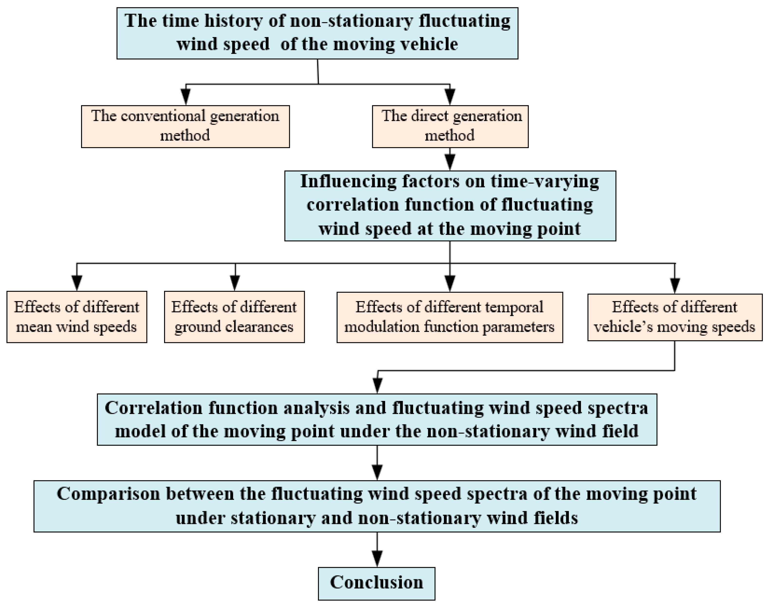
2. Time History of Non-Stationary Fluctuating Wind Speed of the Moving Vehicle

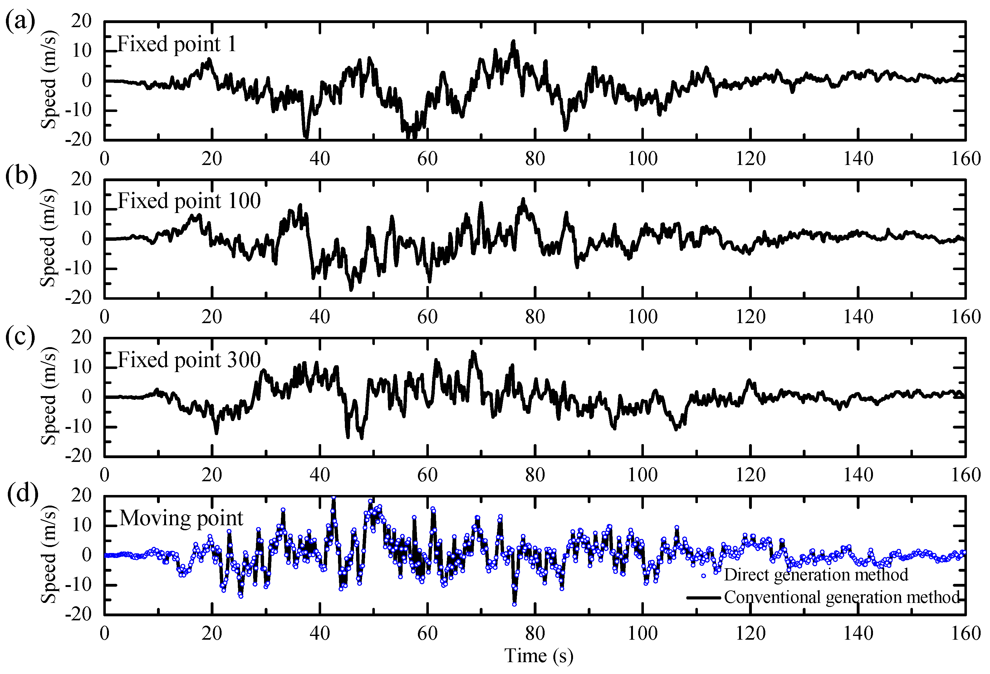
2.1. Time Histories of Non-Stationary Fluctuating Wind Speed at Fixed Points

According to the EPSD theory proposed by Priestley [27], the EPSD matrix for a non-stationary random process {x(t)} = [x₁(t), x₂(t),…, x_n(t)]^T with n variables, zero mean values, and time-invariant coherence can be given as follows [28]:

$$S\left(\omega ,t\right)=\mathrm{D}(\omega ,t\left)\mathsf{\Gamma }\left(\omega \right){\mathrm{D}}^T\right(\omega ,t)$$

(1)

where ω is circular frequency; T is matrix transpose; S(ω, t) is the EPSD of random process x_j(t); Γ(ω) is the coherence matrix; and D(ω, t) and Γ(ω) are given by:

$$\mathrm{D}(\omega ,t)=\mathrm{diag}[\sqrt{S_{11}(\omega ,t)},\sqrt{S_{22}(\omega ,t)},\cdots ,\sqrt{S_{\mathit{nn}}(\omega ,t)}]$$

(2)

$$\mathsf{\Gamma }\left(\omega \right)=\left[\begin{array}{cccc}{\gamma }_{11}\left(\omega \right)& {\gamma }_{12}\left(\omega \right)& \cdots & {\gamma }_{1n}\left(\omega \right)\\ {\gamma }_{21}\left(\omega \right)& {\gamma }_{22}\left(\omega \right)& \cdots & {\gamma }_{2n}\left(\omega \right)\\ ⋮& ⋮& \ddots & ⋮\\ {\gamma }_{n1}\left(\omega \right)& {\gamma }_{n2}\left(\omega \right)& \cdots & {\gamma }_{\mathit{nn}}\left(\omega \right)\end{array}\right]$$

(3)

where γ_jk(ω) is the time-invariant coherence function between x_j(t) and x_k(t). The coherence matrix Γ(ω) is a non-negative definite Hermite matrix and can be decomposed below by Cholesky decomposition:

Γ(ω) = B(ω)B^T*(ω)

(4)

where * denotes complex conjugate, and B(ω) is a lower triangular matrix, which can be given by:

$$B\left(\omega \right)=\left[\begin{array}{cccc}{\beta }_{11}\left(\omega \right)& 0& \cdots & 0\\ {\beta }_{21}\left(\omega \right)& {\beta }_{22}\left(\omega \right)& \cdots & 0\\ ⋮& ⋮& \ddots & ⋮\\ {\beta }_{n1}\left(\omega \right)& {\beta }_{n1}\left(\omega \right)& \cdots & {\beta }_{\mathit{nn}}\left(\omega \right)\end{array}\right]$$

(5)

The following equation can be obtained by Equations (1) and (4):

H(ω, t) = D(ω, t)B(ω)

(6)

As shown in Equation (6), the random process of the time-invariant coherence function only requires decomposition in the frequency domain rather than in both the frequency and time domain, which is decomposed as:

$${\mathrm{H}}_{\mathit{jk}}\left(\omega ,t\right)=\sqrt{S_{\mathit{jj}}\left(\omega ,t\right)}{\beta }_{\mathit{jk}}(\omega ),j=1,2,\dots ,n;j\ge k$$

(7)

The simulation of one random subprocess x_j(t) can be expressed as:

$$x_j\left(t\right)=2\sum _{k=1}^j\sum _{l=1}^N\left|{\mathrm{H}}_{\mathit{jk}}\left({\omega }_l,t\right)\right|\sqrt{\Delta \omega }\cos ({\omega }_{l}t+{\mathsf{\Phi }}_{\mathit{kl}})$$

(8)

where N is the dividing number of frequency; ω_u is the upper cut-off frequency; Δω = ω_u/N is the frequency resolution; ω_l = l Δω, l is an integer; and Φ_kl is uniformly distributed random phase angle with the value interval of [0, 2π].

H_jk(ω_l, t) in Equation (8) fails to improve the simulation efficiency by fast Fourier transform (FFT), as it is only a binary function of time and frequency. Numerous methods have been proposed to improve the simulation efficiency of the non-stationary random process of time-invariant coherence function [28,29]. In this paper, every non-zero element of the lower triangular matrix S_jj(ω, t) is decomposed using the proper orthogonal decomposition (POD) method, and the binary function of time and frequency is decomposed into the sum of the products of time and frequency functions according to the method proposed by Zhao and Huang [30] and Huang [31], which can be expressed as follows:

$$\sqrt{S_{\mathit{jj}}(\omega ,t)}\approx \sum _{q=1}^{N_q^{\mathit{jj}}}{a}_q^{\mathit{jj}}(t){\mathsf{\Phi }}_q^{\mathit{jj}}(\omega ),j=1,2,\dots ,n;j\ge k$$

(9)

where ${\mathsf{\Phi }}_q^{\mathit{jj}}(\omega )$ is the qth feature vector of the frequency correlation matrix; $a_q^{\mathit{jj}}(t)$ is the qth principal coordinates, $a_q^{\mathit{jj}}(t)={[{\mathsf{\Phi }}_q^{\mathit{jj}}(\omega )]}^T{\mathrm{H}}_{\mathit{jj}}(\omega ,t)$; and $N_q^{\mathit{jj}}$ is the number of valid terms with most of the energy. By substituting Equation (9) into Equation (8), the following equation can be obtained:

$$x_j\left(t\right)=\mathrm{Re}\left\{2\sqrt{\Delta \omega }\sum _{q=1}^{N_q^{\mathit{jj}}}{a}_q^{\mathit{jj}}(t)\sum _{l=1}^N{\mathsf{\Phi }}_q^{\mathit{jj}}({\omega }_l)e^{-i{\omega }_{l}t}\sum _{k=1}^j{\beta }_{\mathit{jk}}({\omega }_l)e^{-i{\mathsf{\Phi }}_{\mathit{kl}}}\right\}$$

(10)

The equation above can achieve fast simulation by FFT calculation; N_s wind speed samples only require n times of POD and $N_{\mathrm{s}}\sum _{j=1}^n{N}_q^{jj}$ times of FFT calculation.

The Kaimal spectra are modulated with the uniform temporal modulation function in the non-stationary fluctuating wind speed spectra model, and it is defined as follows [26]:

S(ω, t) = A(t)S(ω)

(11)

$$S(\omega )=\frac{200}{2\mathsf{\pi }}\frac{Z}{U}\frac{u_{*}^2}{{(1+50\frac{\omega Z}{2\mathsf{\pi }U})}^{\frac{5}{3}}}$$

(12)

where Z is the height from the ground; Z₀ is ground roughness; U is the mean wind speed; u_* is the shear velocity (m/s), and u_* = KU/ln(Z/Z₀), with K = 0.4. The temporal modulation function A(t) is a three-parameter function [32], A(t) = αt^β e^−λt, with α > 0, β and λ ≥ 0, α = (λ/βe)^β. The parameters of the temporal modulation function in this paper are taken as β = 4 and λ = 0.08, respectively.

The time-invariant coherence function adopts the coherence function proposed by Shiotani et al. [33], which is only related to the distance between two points. For example, the horizontal lateral coherence function can be expressed as follows:

$$\mathrm{Coh}(\Delta y)=\exp (-\frac{\left|\Delta y\right|}{L_y})$$

(13)

where Δy is the distance between two points, and L_y is the decay coefficient. It is found that the value range of L_y is 40–60 through a large number of experiments, and it is generally taken as L_y = 50.

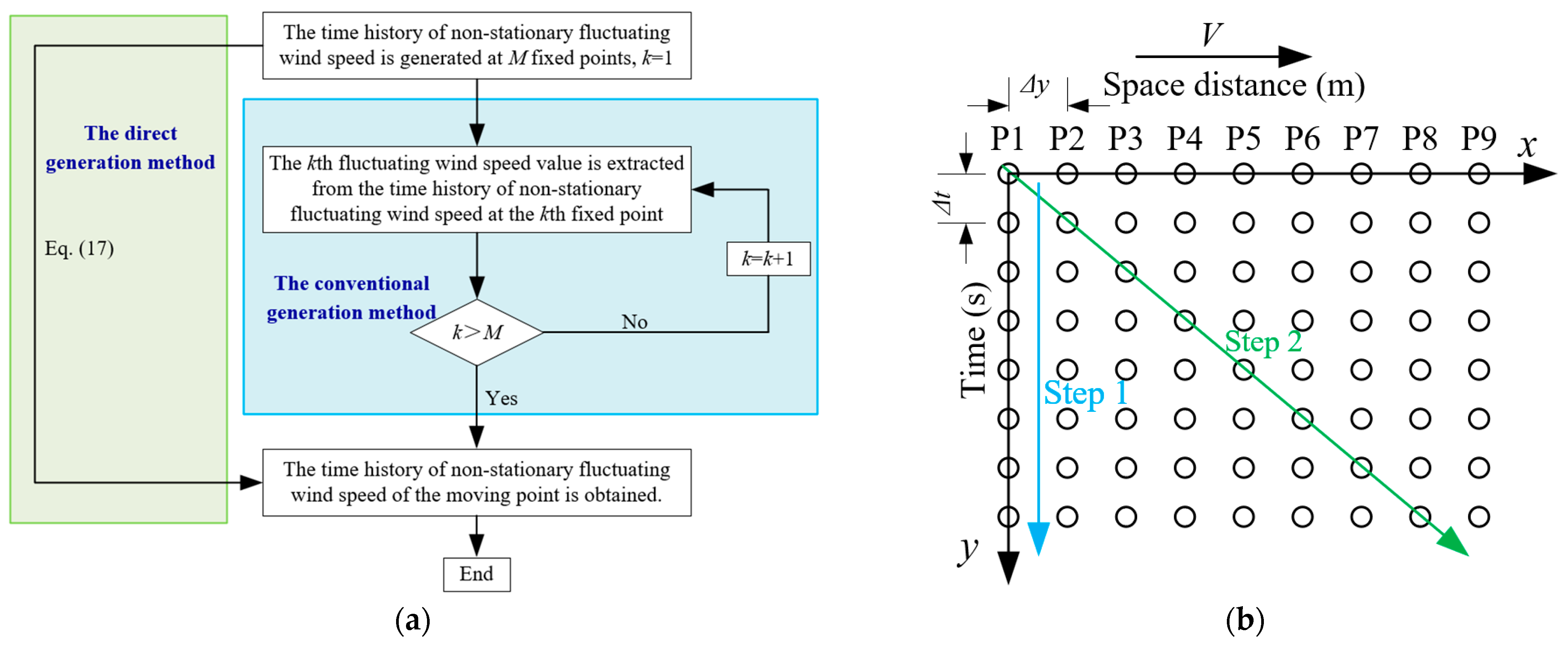
2.2. Time History of Non-Stationary Fluctuating Wind Speed at the Moving Point

The simulation of a non-stationary random process is conducted according to Priestley’s EPSD and Shiotani’s coherence function models. According to a research background that the high-speed train passes over a bridge under the thunderstorm downburst wind field, the parameters are taken as follows: ground clearance Z = 20 m, incoming mean wind speed U = 30 m/s, surface roughness height Z₀ = 0.01 m, sampling time Δt = 0.2 s, dividing number of frequency N = 1024, upper cut-off frequency ω_u = 5π, dividing number of time N_t = 2048, space interval Δy = 8 m, the number of simulated fixed points M = 800, and time of duration is 160 s. The non-stationary fluctuating wind speed time–histories at fixed points are obtained by Equation (10), with the simulated time–history of the 1st, 100th, and 300th points shown in Figure 2a–c. In this paper, N_s = 2000 means that 2000 wind speed samples are generated to estimate the time-varying correlation function and EPSD, which can verify the accuracy of the non-stationary fluctuating wind speeds at fixed points. The estimated results and corresponding target values are shown in Figure 3 and Figure 4, respectively, which show that the correlation function and EPSD of the simulated time history of non-stationary fluctuating wind speed samples at fixed points are both in good agreement with corresponding target values, proving the excellent performance of this method in simulation of non-stationary wind speed time–histories at fixed points.

For simulating the time history of non-stationary fluctuating wind speed at the moving point, the conventional generation method is to extract the wind speed values of corresponding temporal and spatial points from the time–history of non-stationary fluctuating wind speed at fixed points step by step, where the fixed points are points at different positions relative to the ground under the non-stationary wind field. Specifically, the first fluctuating wind speed value is extracted from the time history of non-stationary fluctuating wind speed at the first fixed point, and the second fluctuating wind speed value is extracted from the time history of non-stationary fluctuating wind speed at the second fixed point. By analogy, the kth fluctuating wind speed value is extracted from the time history of non-stationary fluctuating wind speed at the kth fixed point (k is an integer, 1 ≤ k ≤ M). The flow chart for the simulation steps of the conventional generation method is shown in Figure 5a, and the schematic diagram for generating the fluctuating wind speed time history of the moving vehicle is shown in Figure 5b. The hollow dot in the figure represents a fluctuating wind speed value relative to the ground; x is the direction of the moving vehicle, and y is the time. The conventional generating method is to first calculate the fluctuating wind speed time history of each fixed point, as shown in Step 1 in the figure, and then extract a fluctuating wind speed value from each fixed point to obtain the fluctuating wind speed time history of the moving vehicle, as shown in Step 2 in the figure. Then, the extracted time history of non-stationary fluctuating wind speed at the moving point is shown in Figure 2d, where the moving speed of vehicle V is calculated using Δy/Δt = 40 m/s. Obviously, this conventional generation method requires simulating the time history of fluctuating wind speed at each fixed point and then extracting a fluctuating wind speed value from the time histories of each fixed point. In other words, only one fluctuating wind speed value extracted from the time history of non-stationary fluctuating wind speed of each fixed point is used for the time history of non-stationary fluctuating wind speed at the moving point, suggesting a utilization rate of only 1/N_t = 1/2048 = 0.048% for the wind speed series at fixed points mentioned above. This highlights that the conventional generation method is less effective in the establishment of the time history of non-stationary fluctuating wind speed at the moving point.

Based on the research by Hu et al. [34], a direct generation method for the time history of non-stationary fluctuating wind speed of the moving point is proposed here. Accordingly, Equation (13) is mainly changed as follows:

$$\begin{gathered} x_j\left(t\right)=\mathrm{Re}\left\{2\sqrt{\Delta \omega }\sum _{q=1}^{N_q^{\mathit{jj}}}{a}_q^{\mathit{jj}}(t)\sum _{l=1}^N{\mathsf{\Phi }}_q^{\mathit{jj}}({\omega }_l){\mathrm{e}}^{-i{\omega }_{l}t}\sum _{k=1}^j{\beta }_{\mathit{jk}}({\omega }_l){\mathrm{e}}^{-i{\mathsf{\Phi }}_{\mathit{kl}}}\right\} \\ =\mathrm{Re}\left\{\sum _{l=1}^N\sum _{k=1}^{j}2\sqrt{\Delta \omega }\sqrt{S_{\mathit{jj}}({\omega }_l,t)}{\beta }_{\mathit{jk}}({\omega }_l){\mathrm{e}}^{-i{\mathsf{\Phi }}_{\mathit{kl}}}{\mathrm{e}}^{-i{\omega }_{l}t}\right\} \\ =\mathrm{Re}\left\{\sum _{l=1}^N{{\mathrm{H}}_j({\omega }_l,t)\mathrm{e}}^{-i{\omega }_{l}t}\right\} \end{gathered}$$

(14)

where

$${\mathrm{H}}_j\left({\omega }_l,t\right)=2\sqrt{\Delta \omega }\sum _{k=1}^j\sqrt{S_{\mathit{jj}}({\omega }_l,t)}{\beta }_{\mathit{jk}}({\omega }_l){\mathrm{e}}^{-i{\mathsf{\Phi }}_{\mathit{kl}}}$$

(15)

After analysis of the relationship between fluctuating wind speed series at the moving point and fixed points, take t = jΔt, so Equation (14) can be rewritten as:

$$x_j\left(j\Delta t\right)=\mathrm{Re}\left\{\sum _{l=1}^N{{\mathrm{H}}_j({\omega }_l,j\Delta t)\mathrm{e}}^{-i{\omega }_{l}j\Delta t}\right\}$$

(16)

It can be found that x_j(jΔt) is a one-dimensional non-stationary fluctuating wind speed series that only changes with j, so it degenerates into a one-dimensional non-stationary fluctuating wind speed series x(jΔt) and Equation (16) can be simplified as:

$$x\left(j\Delta t\right)=\mathrm{Re}\left\{\sum _{l=1}^N{{\mathrm{H}}_j({\omega }_l,j\Delta t)\mathrm{e}}^{-i{\omega }_{l}j\Delta t}\right\}$$

(17)

Non-stationary fluctuating wind speed series at the moving point can be directly generated by Equations (15) and (17), and such a method is called the direct generation method. Figure 5 also gives the simulation step of the direct generation method; it is seen that the direct generation method can directly generate the fluctuating wind speed time history of the moving vehicle, that is, Step 2 in Figure 5b. Comparison between the direct generation method and conventional generation method shows that the calculation speed of the direct generation method is faster than that of the conventional generation method, one reason for which lies in that the direct generation method does not require POD decomposition and can avoid n times of POD decomposition. On the other hand, the direct generation method does not require $N_{\mathrm{s}}\sum _{j=1}^n{N}_q^{\mathit{jj}}$ times of FFT calculation, while the conventional generation method needs to obtain N_t fluctuating wind speed series of each fixed point using FFT calculation in Equation (10) and then extract a fluctuating wind speed value of the corresponding temporal and spatial point. However, FFT calculation is not needed for simulating the time history of fluctuating wind speed of the moving point using the direct generation method. Therefore, the direct generation method saves more computational memory than the conventional generation method. To verify the correctness of the direct generation method, the time history curves of fluctuating wind speed are, respectively, generated using the direct generation method and the conventional generation method by setting the same parameters, as shown in Figure 2d. It can be seen that the time–history curves of fluctuating wind speed generated using the two methods overlap each other, which verifies the correctness of the direct generation method.

3. Influencing Factors on Time-Varying Correlation Function of Fluctuating Wind Speed at the Moving Point

The correlation function represents the interdependence of two different times in a random process. The comparison between time-varying correlation functions of fluctuating wind speed at fixed and moving points is shown in Figure 6. It indicates that the two function curves coincide well at the time delay τ = 0 s, and the time-varying correlation function of fluctuating wind speed at the moving point is smaller than that at fixed points but with the same variation trend at the time delay τ > 0 s, which will be illustrated and verified in details below. According to Wiener–Khinchin formula and Equations (11) and (12), the transformation relationship between the time-varying correlation function and the EPSD function of the non-stationary random process can be given as follows [35]:

$$\begin{array}{l}R(\tau ,t)={\displaystyle {\int }_0^{+\infty }}S(\omega ,t)\cos (\omega \tau )\mathrm{d}\omega =A(t){\displaystyle {\int }_0^{+\infty }}S(\omega )\cos (\omega \tau )\mathrm{d}\omega \\ =A(t)(6u_{*}^2-\frac{27{\mathsf{\pi }}^2{u}_{*}^2{\gamma }^2}{1250}+\frac{27}{250}{u}_{*}^2{5}^{\frac{2}{3}}{\mathsf{\pi }}^{\frac{7}{6}}{\gamma }^{\frac{7}{6}}\mathrm{LommelS}2(\frac{11}{6},\frac{1}{2},\frac{1}{25}\mathsf{\pi }\gamma ))\end{array}$$

(18)

where R(τ, t) is the time-varying correlation function of the time history of fluctuating wind speed at fixed points, in which τ is the time delay; S(ω, t) is the EPSD function; and γ = τU/Z. LommelS2(p, q, x) is the second kind of the solution of partial differential equation x²y″ + xy′ + (x² − q²)y = x^p+1, the numerical solution of which can be obtained using the mathematical analysis software.

As shown in Equation (18), the time-varying correlation function of fluctuating wind speed at fixed points is related to the temporal modulation function A(t), ground clearance Z, and mean wind speed U. In addition to the three parameters above, the time-varying correlation function of the time history of fluctuating wind speed at the moving point may also be related to the moving speed V. The sensitivity of the four parameters above is analyzed in detail below.

3.1. Effects of Different Mean Wind Speeds

In order to compare the effects of different mean wind speeds on the time-varying correlation function of fluctuating wind speed at the moving point and enhance the contrast under different mean wind speeds, the time–histories of non-stationary fluctuating wind speed at the moving point under the mean wind speeds of 10 m/s, 30 m/s and 50 m/s are generated using the above direct generation method, while other parameters of non-stationary the time history of fluctuating wind speed at moving and fixed points are set as the same as those in Section 2.2. It should be pointed out that the incoming mean wind speeds used here do not mean actual values but for better comparison. The workstation computer equipped with Intel (R) Xeon(R) Gold 6226R CPU @ 2.9 GHz 2.89 GHz and 128 GB RAM is used for computing. Compared with the conventional generating method, the computational efficiency of the direct generation method is increased by 22.7% when generating the wind speed samples. The time-varying correlation functions of fluctuating wind speed at the moving point under different mean wind speeds in Figure 7 represent that the time-varying correlation function values of fluctuating wind speed at moving and fixed points are roughly consistent at the time delay τ = 0 s. When the time delay τ > 0 s, the time-varying correlation function values of fluctuating wind speed at the moving point are smaller than those at fixed points at each time. Meanwhile, the maximum values of the time-varying correlation function of fluctuating wind speed at moving and fixed points increase as the mean wind speed increases. Figure 8 provides the variation of time-varying correlation function ratio between the moving and fixed points over time to further illustrate the relationship between the time-varying correlation function values of non-stationary fluctuating wind speed at moving and fixed points. As indicated in Figure 8, the ratios fluctuate up and down along a line with time, which may be caused by calculation errors. To facilitate data analysis, the ratio of time-varying correlation functions is processed as follows according to its data characteristics: the time-varying correlation functions at different times t are averaged, which then are taken as the final ratio of the two time-varying correlation functions at different time delays τ.

Figure 9 shows the average ratios of time-varying correlation functions of fluctuating wind speed at moving and fixed points under different mean wind speeds, which shows that the average ratio gradually decreases with the increase in time delay τ. More importantly, the average ratios of time-varying correlation functions of fluctuating wind speeds at moving and fixed points are basically coincident under different mean wind speeds, so it can be considered that the ratios do not vary with the change of mean wind speed.

3.2. Effects of Different Ground Clearances

The time–histories of non-stationary fluctuating wind speed at moving and fixed points under the ground clearances of 10 m, 20 m, and 30 m are generated; with the data processed using the same method in Section 3.1, Figure 10 shows the average ratios of time-varying correlation functions of fluctuating wind speed at moving and fixed points under different ground clearances, which also indicates that the average ratio gradually decreases with the increase in time delay τ. More importantly, the average ratios of time-varying correlation functions of fluctuating wind speed at moving and fixed points are basically coincident under different ground clearances, so it can be considered that the ratios do not vary with the change of ground clearances.

3.3. Effects of Different Temporal Modulation Function Parameters

As shown in Equation (11), the temporal modulation function A is a parameter related to λ and β. In order to compare the effects of different temporal modulation function parameters on the time-varying correlation function of fluctuating wind speed at the moving point, the time–histories of non-stationary fluctuating wind speed at the moving point under β = 4 while λ is 0.04, 0.08, 0.12, respectively, and λ = 0.08 while β is 2, 4, and 6, respectively, are generated, with those at fixed points generated as well, while other parameters are set as the same as those in Section 2.2. Figure 11 presents the average ratios between the two under different temporal modulation function parameters λ. It can be seen that the average ratios under different temporal modulation function parameters λ are basically consistent. Therefore, it can be considered that the time-varying correlation function ratio remains unchanged with the change of the temporal modulation function parameter λ.

Similarly, Figure 12 presents the average ratios between the two under different temporal modulation function parameter β. The average ratios are basically coincident under different temporal modulation function parameters β, so it can be considered that the ratios do not vary with the change of temporal modulation function parameter β.

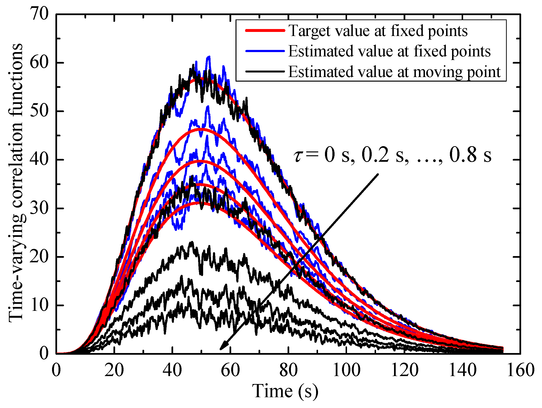
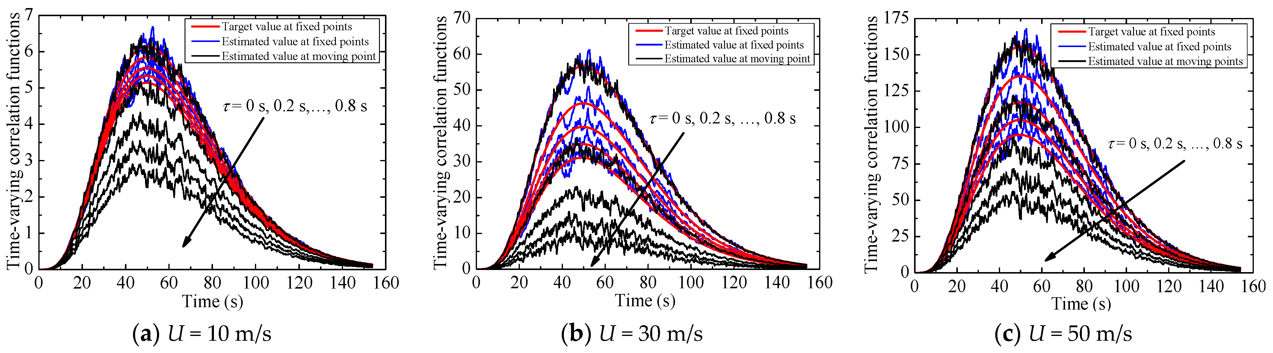
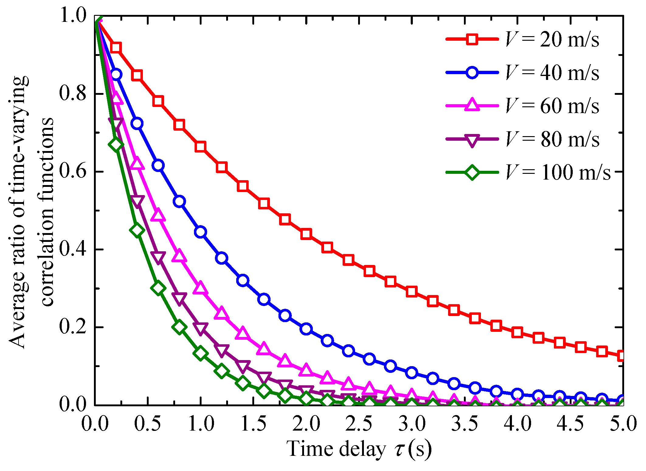
3.4. Effects of Different Vehicle’s Moving Speeds

According to the parameters in Section 2.2, the vehicle’s moving speed V = Δy/Δt = 40 m/s. In order to compare the effects of different vehicle’s moving speeds V on the time-varying correlation functions of fluctuating wind speed at the moving point, the time–history curves of fluctuating wind speed at moving and fixed points under the moving speed V of 20 m/s, 40 m/s, 60 m/s, 80 m/s, and 100 m/s are generated. Figure 13 shows the time-varying correlation functions of fluctuating wind speed at the moving point under different vehicle’s moving speeds. It indicates that the time-varying correlation function values of fluctuating wind speed at moving and fixed points are roughly consistent at the time delay τ = 0 s. However, the time-varying correlation function values of fluctuating wind speed at the moving point are smaller than those at fixed points at each time under the time delay τ > 0 s. Similarly, Figure 14 provides the ratios of time-varying correlation functions between the moving and fixed points at different vehicle’s moving speeds, which shows that the ratios fluctuate up and down along a line over time. However, different from previous sections, the ratios are different at different moving speeds V. Figure 15 shows the average ratios of time-varying correlation functions of fluctuating wind speed at moving and fixed points under different vehicle’s moving speeds V. It is seen that the average ratio between the two gradually decreases with the increase in time delay τ, and the average ratio under the same time delay τ gradually decreases with the increase in vehicle’s moving speed. In a word, the above analysis on the effects of different mean wind speeds, ground clearances, temporal modulation function parameters, and vehicle’s moving speeds on the time-varying correlation function ratios of the time history of fluctuating wind speed at fixed and moving points demonstrate that the ratio of the two is insensitive to mean wind speeds, ground clearances, temporal modulation function parameters, but more sensitive to different vehicle’s moving speeds.

4. Correlation Function Analysis and Fluctuating Wind Speed Spectra Model of the Moving Point under the Non-Stationary Wind Field

4.1. Correlation Function Expression of the Moving Point under the Non-Stationary Wind Field

According to the analysis above, few differences in the time-varying correlation function ratios of the time history of fluctuating wind speed at fixed and moving points are caused by different mean wind speeds, ground clearances, and temporal modulation function parameters, but the ratios are sensitive to different vehicle’s moving speeds. Therefore, it can be concluded that the ratio of the time-varying correlation function of the two is only correlated to the vehicle’s moving speed but uncorrelated to the mean wind speed, ground clearance, and temporal modulation function parameters. Subsequently, a quantitative analysis of the time-varying correlation function of fluctuating wind speed at moving and fixed points is carried out in light of Figure 15. The fitting results of the average ratio of time-varying correlation function between the two under different vehicles’ moving speeds V using the exponential function exp(−bτ) is provided in Figure 16. As indicated in Figure 16, high fitting accuracy is achieved using the exponential function, with the goodness-of-fit parameter R² [36] above 0.999. The changes of parameter b in the exponential function with moving speed V are shown in Figure 17, which reveals that parameter b is basically proportional to the moving speed V, and its relational expression is obtained using linear function fitting as b = 0.02V. Accordingly, the time-varying correlation function of fluctuating wind speed at the moving point R_M(τ, t) and that at fixed points R(τ, t) conform to:

R_M (τ, t) = exp(−0.02 Vτ) R(τ, t)

(19)

4.2. Fluctuating Wind Speed Spectra of the Moving Point under the Non-Stationary Wind Field

According to the Wiener–Khinchin formula, the transformation relationship between the time-varying correlation function and the EPSD function of the non-stationary random process can be given as follows [19]:

$$S(\omega ,t)=\frac{2}{\mathsf{\pi }}{\int }_0^{+\infty }R(\tau ,t)\cos (\omega \tau )\mathrm{d}\tau$$

(20)

The time-varying correlation function of fluctuating wind speed at fixed points by Equation (18) involves special functions and integral calculation of Equation (20), so it can be fitted into the form of exponential function sum to facilitate calculation, with the fitting result shown below:

$$R(\tau ,t)=6u_{*}^{2}A(t)(0.5597\exp (-0.1666\gamma )+0.2943\exp (-1.2237\gamma )+0.1460\exp (-0.0350\gamma ))$$

(21)

The fluctuating wind speed spectra of the moving point under the non-stationary wind field S_M(ω, t) can be obtained by Equations (19)–(21) as:

$$\begin{gathered} S_{\mathrm{M}}(\omega ,t)=\frac{2}{\mathsf{\pi }}{\int }_0^{+\infty }{R}_{\mathrm{M}}(\tau ,t)\cos (\omega \tau )\mathrm{d}\tau =\frac{2}{\mathsf{\pi }}{\int }_0^{+\infty }R(\tau ,t)\exp (-0.02V\tau )\cos (\omega \tau )\mathrm{d}\tau \\ =\frac{{12u}_{*}^{2}A(t)(0.5597A_0+0.2943B_0+0.1460C_0)}{\mathsf{\pi }} \end{gathered}$$

(22)

where

$$A_0=\frac{0.1666K+0.02V}{{(0.1666K+0.02V)}^2+{\omega }^2}$$

(23)

$$B_0=\frac{1.2337K+0.02V}{{(1.2337K+0.02V)}^2+{\omega }^2}$$

(24)

$$C_0=\frac{0.035K+0.02V}{{(0.035K+0.02V)}^2+{\omega }^2}$$

(25)

K = U/Z

(26)

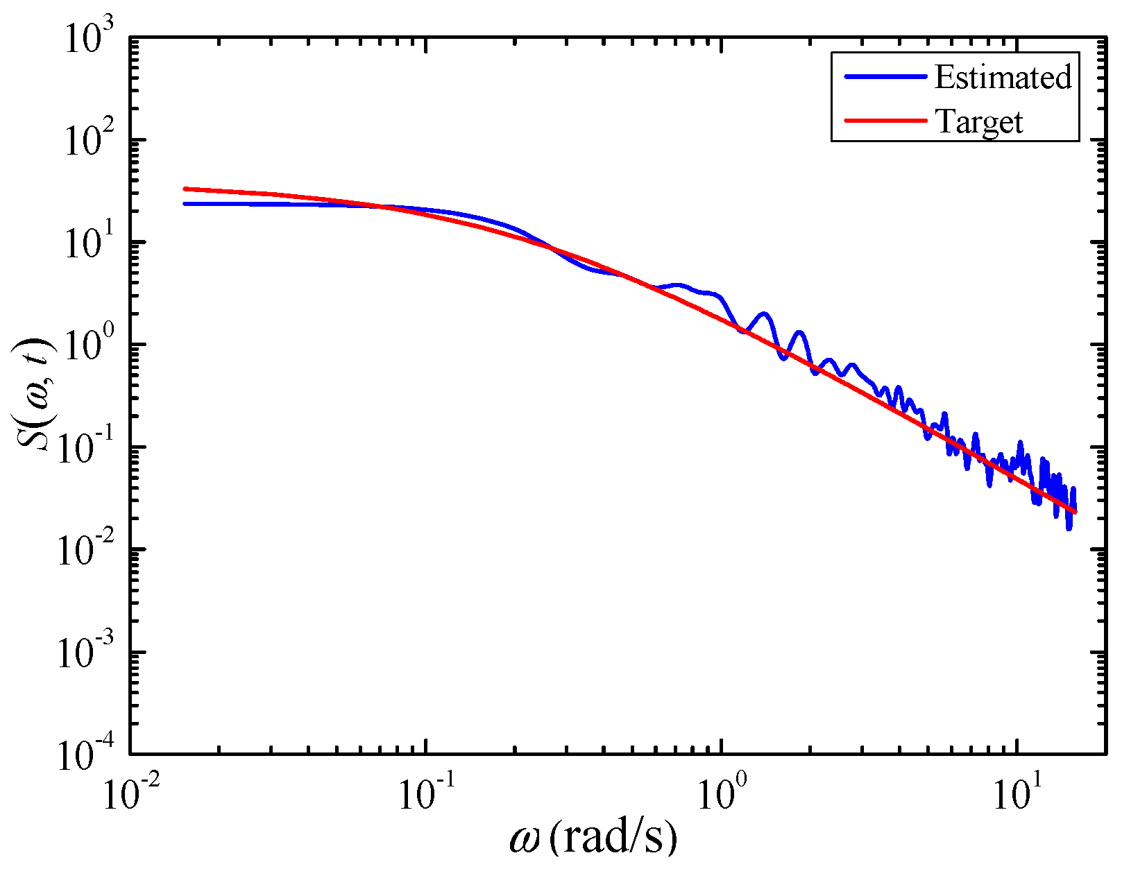
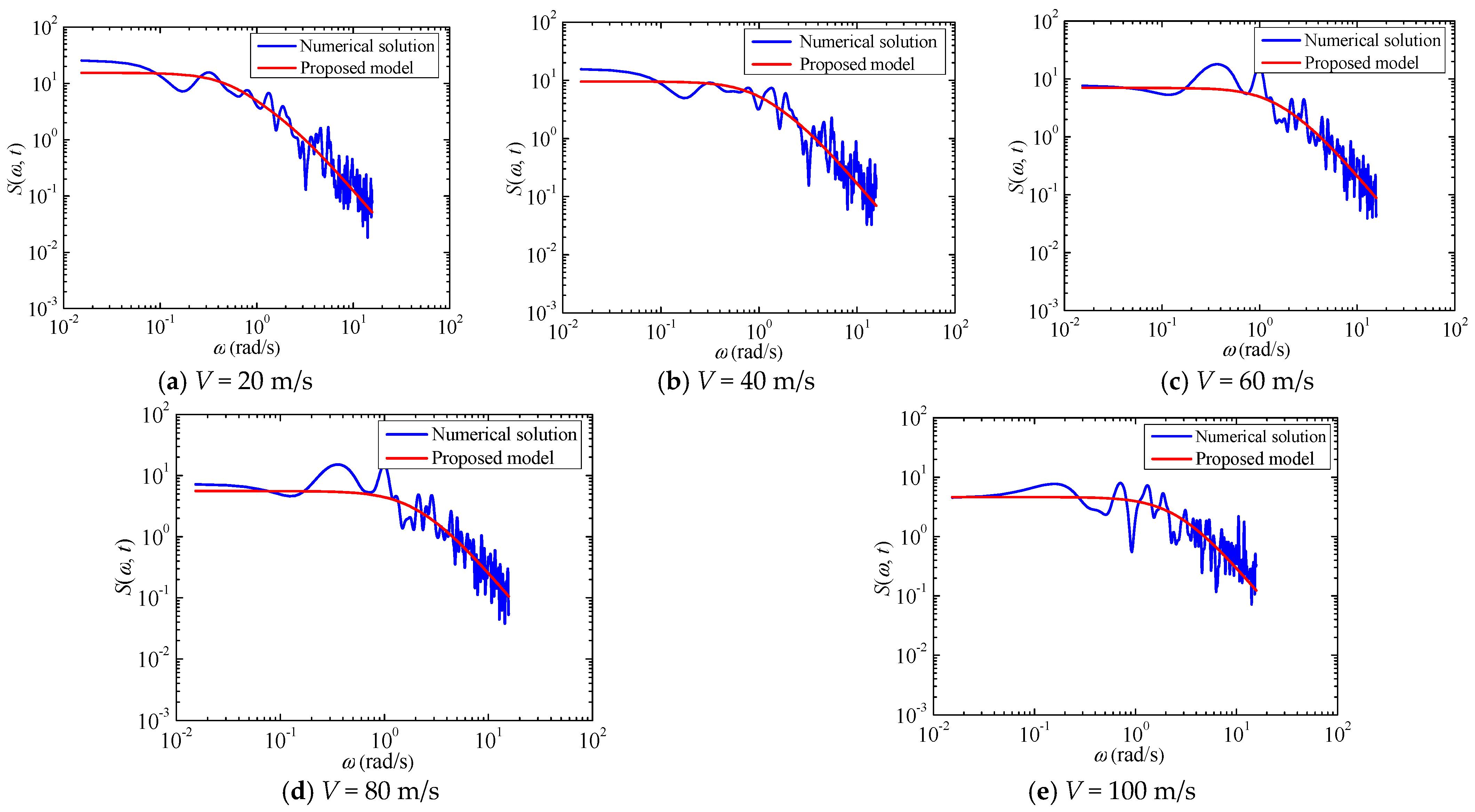
4.3. Verification of Fluctuating Wind Speed Spectra of the Moving Point under the Non-Stationary Wind Field

For the purpose of verifying the correctness of the above-proposed model in calculating the fluctuating wind speed spectra at the moving point under the non-stationary wind field, the numerical solutions of the spectra under the moving speeds of 20 m/s, 40 m/s, 60 m/s, 80 m/s, and 100 m/s are compared with the corresponding calculated values obtained using the proposed model (Equations (22)–(26)), as shown in Figure 18. In regard to the numerical solution, the time history of fluctuating wind speed at the moving point under the non-stationary wind field is generated using the direct generation method with the same parameter settings above, and then the fluctuating wind speed spectra of the moving point under the non-stationary wind field is solved numerically using mathematical software Matlab 2016b. As observed in Figure 18, the calculated values at different moving speeds match well with the corresponding numerical solutions, supporting the high calculation accuracy of the proposed model. In conclusion, the fluctuating wind speed spectra model proposed in this paper by Equations (22)–(26) can simulate the fluctuating wind speed at the moving point under the non-stationary wind field.

5. Comparison between the Fluctuating Wind Speed Spectra of the Moving Point under Stationary and Non-Stationary Wind Fields

5.1. Fluctuating Wind Speed Spectra Model of the Moving Point under the Stationary Wind Field

According to Hu et al. [19], the correlation function and spectra model of fluctuating wind speed at the moving point under the stationary wind field are derived as follows:

$$R_{\mathrm{M}}(\tau )={\int }_0^{\infty }S(\omega )\mathrm{Coh}(V\tau )\cos (\omega \tau )\mathrm{d}\omega$$

(27)

$$S_{\mathrm{M}}(\omega )=\frac{12u_{*}^2(0.5597A_0+0.2943B_0+0.1460C_0)}{\mathsf{\pi }}$$

(28)

where Coh(Vτ) is the coherence function relative to the ground, and other parameters are defined as follows:

$$A_0=\frac{0.1666K+0.02V}{{(0.1666K+0.02V)}^2+{\omega }^2}$$

(29)

$$B_0=\frac{1.2337K+0.02V}{{(1.2337K+0.02V)}^2+{\omega }^2}$$

(30)

$$C_0=\frac{0.035K+0.02V}{{(0.035K+0.02V)}^2+{\omega }^2}$$

(31)

K = U/Z

(32)

Obviously, Equation (22) is similar to Equation (28) except for an additional temporal modulation function A(t). This means that the fluctuating wind speed spectra model at the moving point under the non-stationary wind field can be derived by modulating the model under the stationary wind field with the temporal modulation function, and the temporal modulation function in the fluctuating wind speed spectra model at moving and fixed points keeps the same.

5.2. Fluctuating Wind Speed Spectra Model of the Moving Point under the Non-Stationary Wind Field with Different Modulation Functions

For further verification of the conclusions in Section 5.1, the time-invariant mean wind speed U in Equation (12) is replaced by the time-varying mean wind speed U(t), and the derivation of wind speed spectra model of the moving point under the non-stationary wind field is further carried out, where the time-varying mean wind speed is expressed as follows [37,38]:

U(t) = A(t)U

(33)

where A(t) is the three-parameter temporal modulation function as discussed above, and the EPSD is obtained below by substituting Equation (33) into Equation (12):

$$S(\omega ,t)=\frac{200}{2\mathsf{\pi }}\frac{Z}{U(t)}\frac{u_{*}^2}{{(1+50\frac{\omega Z}{2\mathsf{\pi }U(t)})}^{\frac{5}{3}}}$$

(34)

Hu et al. [19] derived the time-invariant correlation function of the time history of fluctuating wind speed at the moving point under the stationary wind field, as shown in Equation (27), which can also be used to express the time-varying correlation function of the time history of fluctuating wind speed at the moving point under the non-stationary wind field. Obviously, its expression can be written as follows:

$$R_M(\tau ,t)={\int }_0^{\infty }S(\omega ,t)\mathrm{Coh}(V\tau )\cos (\omega \tau )\mathrm{d}\omega$$

(35)

Then, the relational expression of the time-varying correlation functions of fluctuating wind speed at moving and fixed points can be obtained by substituting the Shiotani coherence function by Equation (13) into Equation (35):

R_M(τ, t) = exp(−0.02Vτ)R(τ, t)

(36)

It can be found that Equation (36) is the same as Equation (19), which also proves the accuracy of the above relational expression of the time-varying correlation functions of fluctuating wind speed time–histories at moving and fixed points under the non-stationary wind field obtained by the numerical analysis. Meanwhile, R_M (0, t) = R (0, t) at the time delay τ = 0, and R_M (τ, t) > R (τ, t) at the time delay τ > 0 can also be observed. In other words, under different mean wind speeds, ground clearances, temporal modulation function parameters, and vehicle’s moving speeds, the time-varying correlation function values of fluctuating wind speed at fixed and moving points are identical at the time delay τ = 0 s, while the time-varying correlation function values of fluctuating wind speed at the moving point are smaller than those at fixed points at each time under the time delay τ > 0 s, which also explains why the time-varying correlation function values of fluctuating wind speed at moving and fixed points vary at different time delay τ in Section 3.

By Substituting Equations (34) and (13) into Equation (36), the following equation can be obtained:

$$R_{\mathrm{M}}(\tau ,t)=\exp (-\frac{V\tau }{50})\left[6u_{*}^2-\frac{27{\mathsf{\pi }}^2{u}_{*}^2{{\gamma }_1}^2}{1250}+\frac{27}{250}{u}_{*}^2{5}^{\frac{2}{3}}{\mathsf{\pi }}^{\frac{7}{6}}{{\gamma }_1}^{\frac{7}{6}}\mathrm{LommelS}2(\frac{11}{6},\frac{1}{2},\frac{1}{25}\mathsf{\pi }{\gamma }_1)\right]$$

(37)

where γ₁ = τU(t)/Z = τA(t)U/Z.

Equation (37) is fitted into the form of an exponential function sum with the same fitting method as discussed above, as shown below:

$$R_{\mathrm{M}}(\tau ,t)=6u_{*}^2\exp (-0.02V\tau )\left[0.5597\exp (-0.1666{\gamma }_1)+0.2943\exp (-1.2237{\gamma }_1)+0.1460\exp (-0.0350{\gamma }_1)\right]$$

(38)

According to the Wiener–Khinchin formula, the fluctuating wind speed spectra of the moving point under the non-stationary wind field can be obtained as:

$$S_{\mathrm{M}}(\omega ,t)=\frac{{12u}_{*}^2(0.5597A_1+0.2943B_1+0.1460C_1)}{\mathsf{\pi }}$$

(39)

where

$$A_1=\frac{0.1666K_1+0.02V}{{(0.1666K_1+0.02V)}^2+{\omega }^2}$$

(40)

$$B_1=\frac{1.2337K_1+0.02V}{{(1.2337K_1+0.02V)}^2+{\omega }^2}$$

(41)

$$C_1=\frac{0.035K_1+0.02V}{{(0.035K_1+0.02)}^2+{\omega }^2}$$

(42)

K₁ = A(t)U/Z

(43)

For the purpose of verifying the correctness of the model above in calculating the fluctuating wind speed spectra at the moving point under the non-stationary wind field, the numerical solution of the spectra is compared with the corresponding calculated values obtained by Equations (39)–(43), as shown in Figure 19. It is seen that the calculated values of the model match well with the corresponding numerical solution, supporting the high calculation accuracy of the model by Equations (39)–(43).

Obviously, Equation (39) is similar to Equation (28), except for an additional temporal modulation function A(t) in the parameter K₁ in Equation (39) as compared to the K in Equation (28). This lies in that the above EPSD is obtained by modulating the mean wind speed in Kaimal spectra by the temporal modulation function (Equation (33)), which again proves that the fluctuating wind speed spectra model at the moving point under the non-stationary wind field can be derived using modulating the model under the stationary wind field with the temporal modulation function. Furthermore, the temporal modulation function in the fluctuating wind speed spectra model at moving and fixed points remains the same. It should be noted that the modulation function here only involves a temporal modulation function without a frequency modulation component.

6. Conclusions

Focusing on the generation method of the time history of fluctuating wind speed for the moving vehicle under the non-stationary wind field, this paper proposed a fluctuating wind speed spectra model of the moving vehicle under the non-stationary wind field based on Priestley’s EPSD theory, with the main conclusions listed as follows:

(1)

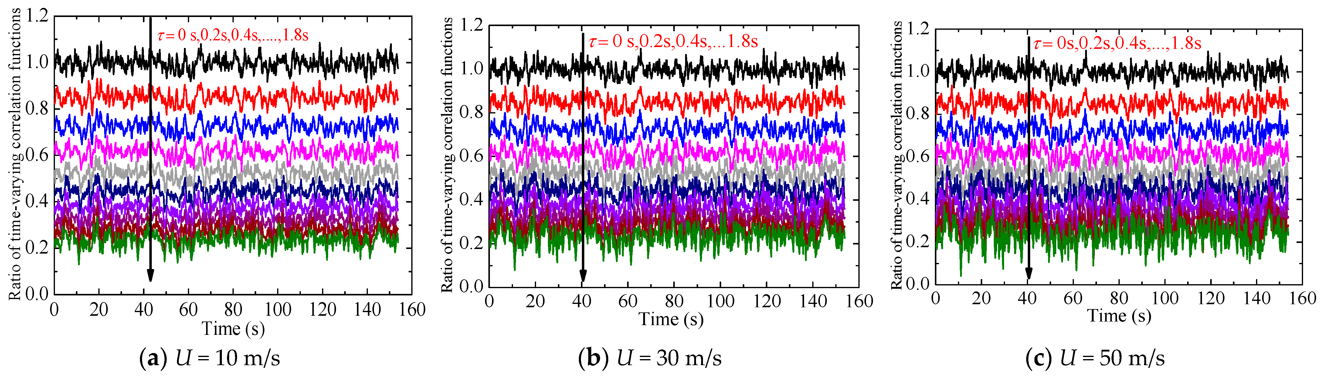
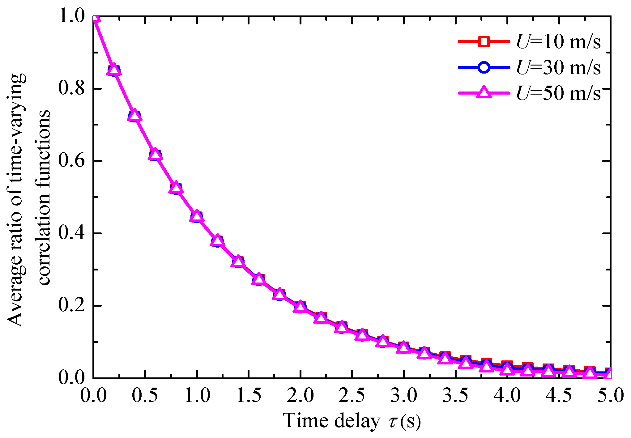
Compared with different mean wind speeds, ground clearances, and temporal modulation function parameters, different vehicles’ moving speeds are more sensitive to the time-varying correlation function ratios of moving and fixed points under the non-stationary wind field.

(2)

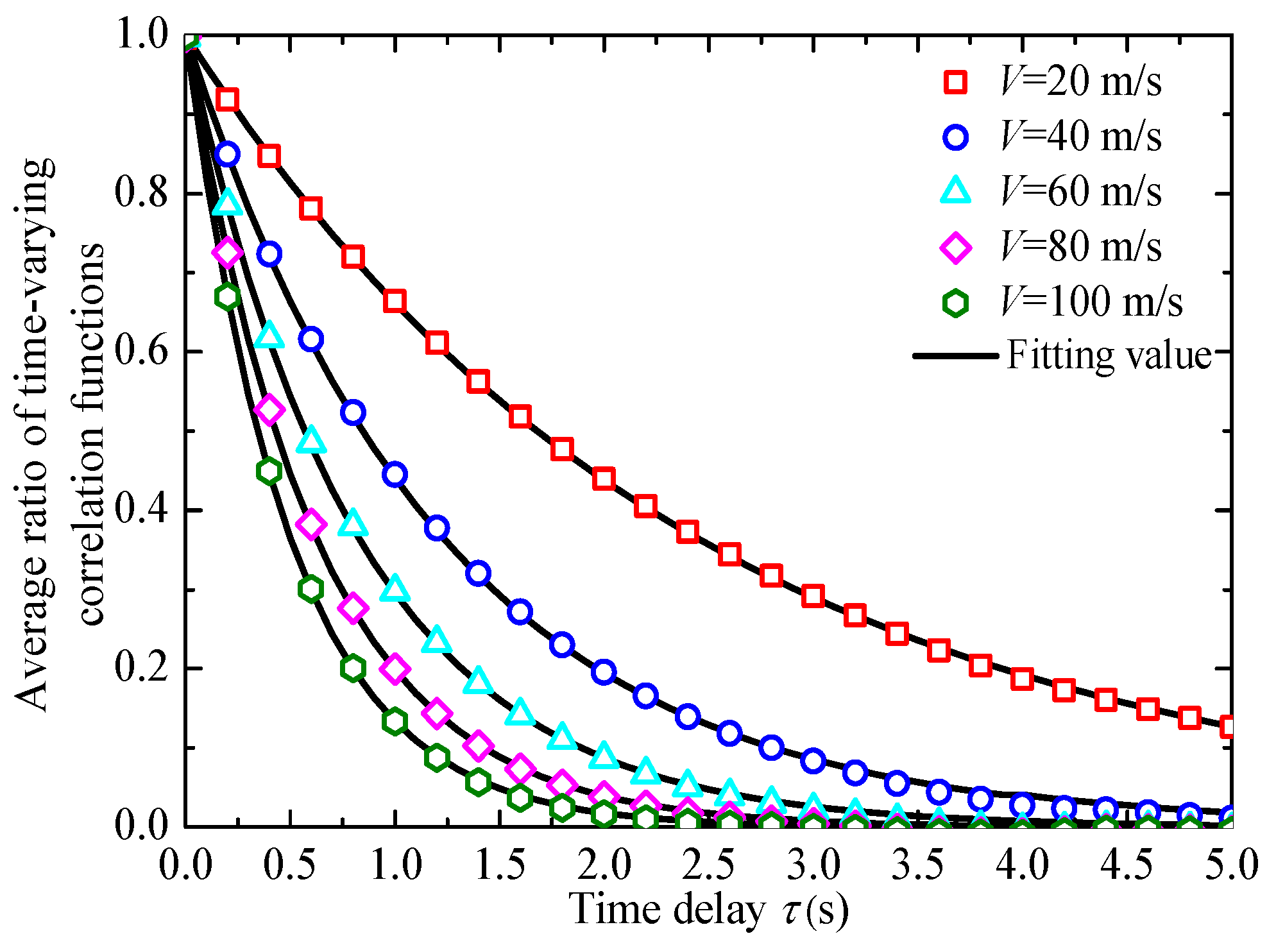
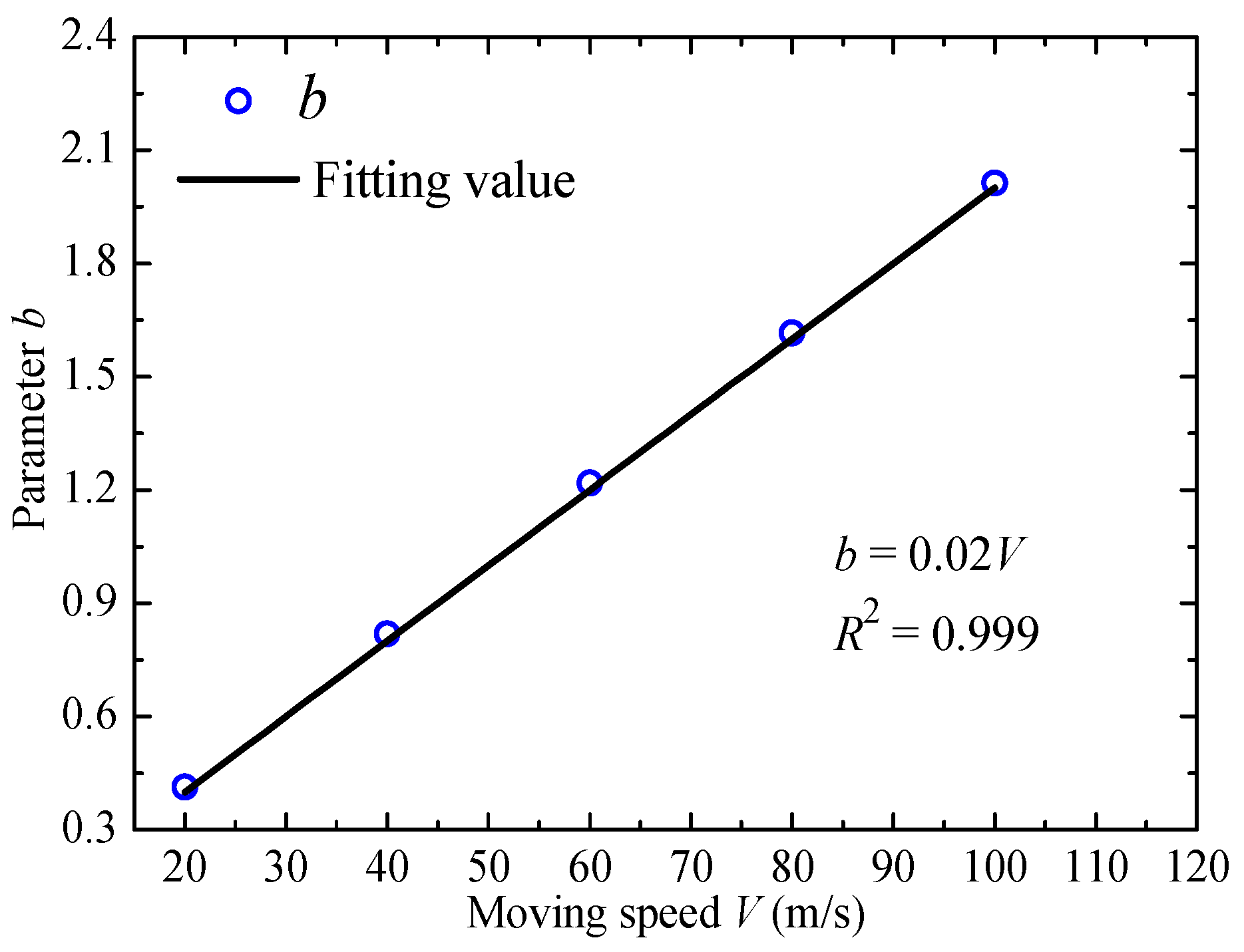
Based on the analysis of the time-varying correlation function ratios between moving and fixed points, the relational expression of the time-varying correlation functions of the time history of fluctuating wind speed at the moving and fixed points are established and the expression of the time-varying correlation function of the moving point under the non-stationary wind field is derived. Furthermore, the fluctuating wind speed spectra model of the moving point under the non-stationary wind field is proposed.

(3)

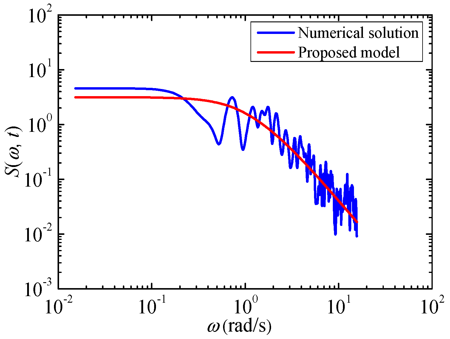
The comparison supports the accuracy of the proposed fluctuating wind speed spectra model at the moving point under the non-stationary wind field by demonstrating good agreement between the calculated values of the fluctuating wind speed spectra model at different vehicle moving speeds and the corresponding target numerical solutions.

(4)

The temporal modulation function of the fluctuating wind speed spectra at the moving point is found to be identical to that at fixed points under the non-stationary wind field.

References

1. Szuzki, M.; Tanemoto, K.; Maeda, T. Aerodynamic Characteristics of Train/Vehicles under Cross Winds. J. Wind Eng. Ind. Aerodyn. 2003, 91, 209–218. [Google Scholar] [CrossRef]
2. Ge, S.C.; Jiang, F.Q. Analyses of the Causes for Wind Disaster in Strong Wind Area Along Lanzhou-Xinjiang Railway and the Effect of Wind-break. J. Railw. Eng. Soc. 2009, 128, 1–4. [Google Scholar]
3. Ge, S.C.; Yin, Y.S. Field Test Study on Train Safety Operation Standard in Xinjiang Railway Wind Area. Railw. Qual. Control 2006, 34, 9–11. [Google Scholar]
4. Baker, C.J. A framework for the consideration of the effects of crosswinds on trains. J. Wind Eng. Ind. Aerodyn. 2013, 123, 130–142. [Google Scholar] [CrossRef]
5. Montenegro, P.; Carvalho, H.; Ortega, M.; Millanes, F.; Goicolea, J.; Zhai, W.; Calçada, R. Impact of the train-track-bridge system characteristics in the runnability of high-speed trains against crosswinds—Part I: Running safety. J. Wind Eng. Ind. Aerodyn. 2022, 224, 104974. [Google Scholar] [CrossRef]
6. Yan, N.; Chen, X.; Li, Y. Assessment of overturning risk of high-speed trains in strong crosswinds using spectral analysis approach. J. Wind Eng. Ind. Aerodyn. 2018, 174, 103–118. [Google Scholar] [CrossRef]
7. Zhou, Y.; Chen, S. Fully coupled driving safety analysis of moving traffic on long-span bridges subjected to crosswind. J. Wind Eng. Ind. Aerodyn. 2015, 143, 1–18. [Google Scholar] [CrossRef]
8. Zheng, Q.P. Jing hu high-speed railway and environment at protection. J. Railw. Eng. Soc. 1998, 1, 12–19. [Google Scholar]
9. Xu, X.C.; Liu, J.M.; Ma, J.; Zhang, C.; Zhang, J.Y.; Li, G. Discussion of environment impacts characters of the high speed railway. Railw. Energy Sav. Environ. Prot. Occup. Saf. Health 2012, 2, 117–121. [Google Scholar]
10. Cornet, Y.; Dudley, G.; Banister, D. High Speed Rail: Implications for carbon emissions and biodiversity. Case Stud. Transp. Policy 2018, 6, 376–390. [Google Scholar] [CrossRef]
11. Su, X.C.; Ma, Y.F.; Wang, L.; Guo, Z.Z.; Zhang, J.R. Fatigue life prediction for prestressed concrete beams under corrosion deterioration process. Structures 2022, 43, 1704–1715. [Google Scholar] [CrossRef]
12. Ma, Y.F.; Peng, A.Y.; Wang, L.; Zhang, C.Z.; Li, J.; Zhang, J.R. Fatigue performance of an innovative shallow-buried modular bridge expansion joint. Eng. Struct. 2020, 221, 111107. [Google Scholar] [CrossRef]
13. Davenport, A.G.; Agnew, R.; Harris, R.I.; Sachs, P. The application of statistical concepts to the wind loading of structures. Proc. Inst. Civil. Eng. Lond. 1961, 19, 449–472. [Google Scholar] [CrossRef]
14. Davenport, A.G. The spectrum of horizontal gustiness near the ground in high winds. Q. J. R. Meteorol. Soc. 1962, 88, 197–198. [Google Scholar] [CrossRef]
15. Balzer, L.A. Atmospheric turbulence encountered by high-speed ground transport vehicles. J. Mech. Eng. Sci. 1977, 19, 227–235. [Google Scholar] [CrossRef]
16. Cooper, R.K. Atmospheric turbulence with respect to moving ground vehicles. J. Wind Eng. Ind. Aerodyn. 1984, 17, 215–238. [Google Scholar] [CrossRef]
17. Wu, M.; Li, Y.; Chen, X.; Hu, P. Wind spectrum and correlation characteristics relative to vehicles moving through cross wind field. J. Wind Eng. Ind. Aerodyn. 2014, 133, 92–100. [Google Scholar] [CrossRef]
18. Li, X.-Z.; Xiao, J.; Liu, D.-J.; Wang, M.; Zhang, D.-Y. An analytical model for the fluctuating wind velocity spectra of a moving vehicle. J. Wind Eng. Ind. Aerodyn. 2017, 164, 34–43. [Google Scholar] [CrossRef]
19. Hu, P.; Han, Y.; Cai, C.S.; Cheng, W.; Lin, W. New analytical models for power spectral density and coherence function of wind turbulence relative to a moving vehicle under crosswinds. J. Wind Eng. Ind. Aerodyn. 2019, 188, 384–396. [Google Scholar] [CrossRef]
20. Chen, L.; Letchford, C.W. A deterministic–stochastic hybrid model of downbursts and its impact on a cantilevered structure. Eng. Struct. 2004, 26, 619–629. [Google Scholar] [CrossRef]
21. Holmes, J.D.; Oliver, S.E. An empirical model of a downburst. Eng. Struct. 2000, 22, 1167–1172. [Google Scholar] [CrossRef]
22. Wood, G.S.; Kwok, K.C.S.; Motteram, N.A.; Fletcher, D.F. Physical and numerical modelling of thunderstorm downdraft. J. Wind Eng. Ind. Aerodyn. 2001, 89, 535–552. [Google Scholar] [CrossRef]
23. Wang, H.; Wu, T.; Tao, T.; Li, A.; Kareem, A. Measurements and analysis of non-stationary wind characteristics at Sutong Bridge in Typhoon Damrey. J. Wind Eng. Ind. Aerodyn. 2016, 151, 100–106. [Google Scholar] [CrossRef]
24. Wang, H.; Li, A.Q.; Niu, J.; Zong, Z.; Li, J. Long-term monitoring of wind characteristics at Su Tong Bridge site. J. Wind Eng. Ind. Aerodyn. 2013, 115, 39–47. [Google Scholar] [CrossRef]
25. Ding, Y.L.; Zhou, G.D.; Li, W.H.; Wang, X.J.; Yan, X. Nonstationary analysis of wind-induced responses of bridges based on evolutionary spectrum theory. China J. Highw. Transport. 2013, 26, 54–61. [Google Scholar]
26. Huang, G.; Zheng, H.; Xu, Y. Spectrum models for nonstationary extreme winds. J. Struct. Eng. 2015, 141, 04015010. [Google Scholar] [CrossRef]
27. Priestley, M.B. Evolutionary spectra and non-stationary processes. J. R. Stat. Soc. B 1965, 27, 204–237. [Google Scholar] [CrossRef]
28. Li, Y.; Kareem, A. Simulation of multivariate nonstationary random processes by FFT. J. Eng. Mech ASCE 1991, 117, 1037–1058. [Google Scholar] [CrossRef]
29. Huang, G. An efficient simulation approach for multivariate random process: Hybrid of wavelet and spectral representation method. Probab. Eng. Mech. 2014, 37, 74–83. [Google Scholar] [CrossRef]
30. Zhao, N.; Huang, G. Fast simulation of multivariate nonstationary process and its application to extreme winds. J. Wind Eng. Ind. Aerodyn. 2017, 170, 118–127. [Google Scholar] [CrossRef]
31. Huang, G. Application of proper orthogonal decomposition in fast Fourier transform-assisted multivariate nonstationary process simulation. J. Eng. Mech. ASCE 2015, 141, 04015015. [Google Scholar] [CrossRef]
32. Huang, G.; Liao, H.; Li, M. New formulation of Cholesky decomposition and applications in stochastic simulation. Probab. Eng. Mech. 2013, 34, 40–47. [Google Scholar] [CrossRef]
33. Shiotani, M. Correlations of wind velocities in relation to the gust loadings. In Proceedings of the Third International Conference on Wind Effects on Buildings and Structures; Saikon, Co.: Tokyo, Japan, 1971. [Google Scholar]
34. Hu, P.; Lin, W.; Yang, D.; Yan, H.; Cong, Y. Fluctuation wind speed spectrum of a moving vehicle under crosswinds. China J. Highw. Transp. 2018, 31, 101–109. [Google Scholar]
35. Bendat, J.S.; Piersol, A.G. Random Data: Analysis and Measurement Procedures; Wiley: New York, NY, USA, 2000. [Google Scholar]
36. Originlab Corporation. Origin Reference for Origin 8.5 SR1; Originlab Corporation: Northampton, UK, 2010. [Google Scholar]
37. Chen, X. Analysis of alongwind tall building response to transient nonstationary winds. J. Struct. Eng. 2008, 134, 782–791. [Google Scholar] [CrossRef]
38. Zhao, N.; Huang, G. Wind velocity field simulation based on enhanced closed-form solution of Cholesky decomposition. J. Eng. Mech. 2020, 146, 04019128. [Google Scholar] [CrossRef]
Figure 1. The studied configuration of this paper.
Sustainability 15 12901 g001
Figure 2. Time histories of fluctuating wind speed at the fixed and moving points. (a) Fixed point 1; (b) Fixed point 100; (c) Fixed point 300; (d) Moving point.
Sustainability 15 12901 g002
Figure 3. Time-varying correlation function of fluctuating wind speed at a fixed point (Taking point 1 as an example).
Sustainability 15 12901 g003
Figure 4. EPSD of a fixed point (Taking point 1 as an example).
Sustainability 15 12901 g004
Figure 5. The simulation step of the conventional generation method and direct generation method. (a) Flow chart for simulation steps of conventional generation method and direct generation method. (b) The schematic diagram for generating the fluctuating wind speed time history of the moving vehicle.
Sustainability 15 12901 g005
Figure 6. Comparison between time-varying correlation functions of fluctuating wind speed at fixed and moving points.
Sustainability 15 12901 g006
Figure 7. Time-varying correlation functions of fluctuating wind speed at moving and fixed points under different mean wind speeds.
Sustainability 15 12901 g007
Figure 8. Ratios of time-varying correlation functions of fluctuating wind speed at moving and fixed points under different mean wind speeds.
Sustainability 15 12901 g008
Figure 9. Average ratio of time-varying correlation functions of fluctuating wind speed at moving and fixed points under different mean wind speeds.
Sustainability 15 12901 g009
Figure 10. Average ratio of time-varying correlation functions of fluctuating wind speed at moving and fixed points under different ground clearances.
Sustainability 15 12901 g010
Figure 11. Average ratio of time-varying correlation functions of fluctuating wind speed at moving and fixed points under different temporal modulation function parameter λ.
Sustainability 15 12901 g011
Figure 12. Average ratio of time-varying correlation functions of fluctuating wind speed at moving and fixed points under different temporal modulation function parameter β.
Sustainability 15 12901 g012
Figure 13. Time-varying correlation functions of fluctuating wind speed at moving and fixed points under different vehicle’s moving speeds.
Sustainability 15 12901 g013
Figure 14. Ratios of time-varying correlation functions of fluctuating wind speed at moving and fixed points under different vehicles’ moving speeds.
Sustainability 15 12901 g014aSustainability 15 12901 g014b
Figure 15. Average ratio of time-varying correlation functions of fluctuating wind speed at moving and fixed points under different vehicle’s moving speeds.
Sustainability 15 12901 g015
Figure 16. Fitting results of average ratio of time-varying correlation functions of fluctuating wind speed at moving and fixed points under different vehicle’s moving speeds.
Sustainability 15 12901 g016
Figure 17. Fitting results of parameter b.
Sustainability 15 12901 g017
Figure 18. Comparison of calculated values with numerical solutions of fluctuating wind speed spectra at the moving point under the non-stationary wind field (t = 150 s).
Sustainability 15 12901 g018
Figure 19. Comparison of calculated values with numerical solutions of fluctuating wind speed spectra at the moving point under the non-stationary wind field with different modulation functions (t = 150 s).
Sustainability 15 12901 g019
Disclaimer/Publisher’s Note: The statements, opinions and data contained in all publications are solely those of the individual author(s) and contributor(s) and not of MDPI and/or the editor(s). MDPI and/or the editor(s) disclaim responsibility for any injury to people or property resulting from any ideas, methods, instructions or products referred to in the content.