Assessment of Land Surface Temperature from the Indian Cities of Ranchi and Dhanbad during COVID-19 Lockdown: Implications on the Urban Climatology

Abstract

An apparent increase in average global temperature is evident globally, and India is no exception. With the recent decade (2011–2020) arguably being the warmest, significant challenges due to rapid climate change have gained attention. However, notable spatial-temporal changes, especially with regard to land surface temperature (LST), were observed during the COVID-19 pandemic lockdown period, when a comparatively cooler climate was experienced in many urban centers. Assessment of LST, crucial in many heat-balance, land use, and climate change models research studies, depicts the near-surface hotness of the Earth’s temperature at a given location. Thus, this study utilizes satellite remote-sensing data to investigate the spatial-temporal variations of LST pre and post-lockdown imposed during the COVID-19 outbreak. Unlike many existing research studies on the metropolitans of India, the study considers developing Indian cities, Ranchi and Dhanbad, as its study area. Accurate LST computation was performed using existing LANDSAT-8 OLI/TIRS images and judged using other parameters (NDVI, LSE) obtained directly from the thermal infrared bands. The LST assessment successfully estimated temperature variations in Ranchi and Dhanbad, depicting a significant drop in temperature coinciding with the lockdown period and subsequent increase in urban temperature post-pandemic, indicating a meaningful relationship between human activities and urban surface temperature.

1. Introduction

South Asian countries are vulnerable to natural disasters [1,2,3], and various scientists have worked on schemes for mitigating the impact of the disaster [4,5,6,7,8]. A high death toll and economic and infrastructural damages from natural disasters are not only linked to the event’s severity; an ignorance of scientific facts and uncontrolled urban sprawl also contribute to the misery [9,10]. Unprecedented growth in urban settlements has occurred in the past decade due to rapid urbanization. Approximately 50% of the global populace resides in urban centers, with estimates indicating a further rise in this figure in the coming years [11,12,13]. An increase in migration [14] and improved life expectancy due to better opportunities and healthcare frameworks in urban localities have contributed to the exponential population growth at a higher rate than in rural settlements leading to unplanned development of cities, particularly in emerging nations. The expected population growth forecasts that 6.3 billion people, or 70% of the predicted 9.1 billion globally by 2050, will live in urban areas [15,16]. Urban populations have presented a snowball scenario in Africa and Asia during the past 70 years, outnumbering Europe, North, and Latin America. In 1950, less than 20% of Africans and Asians resided in urban areas; by 2020, those numbers increased to 43% and 51%, respectively [17,18]. South America’s urban population grew significantly during this time, surpassing Europe’s urban population share by more than 80% [19,20]. India, with approximately 1.4 billion inhabitants, now has 377.1 million, accounting for 36% of the total population, living in urban settlements resulting in extensive changes to its land usage [21].

Transforming naturally permeable land surfaces into artificial built-up surfaces is the most significant alteration urban growth brings [22,23]. Moreover, NDVI, Pv measures the vegetation density, “Land-cover” (LC), and “land-use” (LU), phrases used interchangeably, imply to indicate the categorization of human activities and natural features on the landscape through time, broadly encompasses; flora, urban infrastructure, water bodies, etc. Additionally, changes in LULC, primarily caused by urbanization, substantially impact the local temperature, hydrogeological conditions, and environmental sustainability [24,25]. The surface energy balance in urban areas changes because of alterations in land surface characteristics [26,27], indicating that urbanization will further trigger the expansion in the geographic extent, significantly changing the LU-LC pattern, and shall be primarily responsible for the environmental degradation [28] while also influencing LST, which determines the UHI of the environment [26]. LST, a broad term for climatic variable, is a relative measure of temperature one meter above the lithosphere [29] and is among the crucial parameters to examine the surface UHI [26,30], which governs the near-surface energy equilibrium state and the influences surface heat redistribution, which subsequently influences cities microclimate [31]. LST derived from various remotely sensed data sources is extensively utilized for identifying and characterizing UHI and ecological comfort zones [32].

Furthermore, the UHI phenomenon, also known as urban heat island, refers to higher temperatures in urban areas than in the surrounding rural areas [33,34,35]. This effect is caused by higher thermal mass and greater heat absorption, storage, and release capacity in urban areas than in rural areas [36]. In general, the two main approaches for measuring UHIare; (i) The subsurface urban heat island (SUHI) and (ii) forest/canopy layer heat island (CLHI). The difference in ground temperature observed simultaneously between the metropolitan area and its peri-urban vicinity, i.e., (LSTurban—LSTrural) [37,38], is known as the SUHI intensity. It is accepted mainly for spatiotemporal research studies.

The intensity of LST and SUHI spatially varies dramatically owing to the extensive homogeneity of LC in small heterogeneous metropolitan regions or huge homogenous rural surfaces [29]. Additionally, various LULC types respond differently in the TIR band, resulting in a wide range of LST datasets in an urban landscape [39]. Furthermore, LST spatial and temporal data vary during the day (often higher during the day than at night) because of the influence of ultraviolet irradiance on climatic change [40]. They are also heavily impacted by urban surface features [41], i.e., the amount of vegetation cover, water bodies, and impermeable anthropogenic surfaces. Moreover, a similar variation trend in data was noticed with (i) seasonal changes since sun altitudes and azimuths fluctuate with seasons and (ii) atmospheric phenomena (typology, wind, urban ventilation, infrastructures, building materials, moisture, radiant and aerodynamics) which are sensitive and typically considered as localized phenomena. Time, season, and region-specific microclimate fluctuations are crucial factors in LST monitoring [42,43].

Since the beginning of the century, it has been observed that the average temperature of the Earth has risen by 0.6 °C. LST is anticipated to climb by 1.4 °C–5.8 °C globally as CO₂ levels ramp up, approximately twice from current levels as anticipated by IPCC (Intergovernmental Panel on Climate Change) [26,28]. Furthermore, numerous urban environmental issues or climatic parameters, like UHI, LST, Albedo, and LC changes, are directly or indirectly related to urbanization [44] and are responsible for global temperature rise. The heat significantly impacts the local climate, public health, quality of life, and energy use, most noticeable at night and when there is cloud cover. Urban canyons and substituting vegetative land covers with impervious surfaces (resulting from urbanization) have reduced the evapotranspiration rates and increased latent heat due to the thermal properties of various construction materials [26,45]. Thus, the anthropogenic heat generated from manufacturing facilities, chemicals, air conditioners, coolants, and motor vehicles [44,46] influences UHI’s dynamics changing the airflow and contributing to the local micro-climate [47]. UHI exacerbates airflow declination and is a distinct indicator of environmental deterioration [48,49].

Moreover, the impact of degraded thermal surroundings has thus resulted in increased morbidity and mortality [30,50]. LST and UHI generate a variety of socioeconomic, environmental, and climatic issues that harms or restrict biodiversity, energy balance, regional and urban climate [51,52,53], quality of air and water [37,54], and energy costs [55]. As such, climate change, unfavorable weather conditions (increased surface temperature), and heat waves in the urban setting brought on by the combined effects of UHI and global warming due to outrageous GHG emissions have resulted in precarious circumstances for urban communities [54] making climate change-brought catastrophes seemed inevitable for developing nations like India.

Despite the Corona-Virus pandemic’s detrimental effects on the global economy [56,57,58] and massive human mortality rate [59,60], it envisaged preventive measures such as travel bans and mass quarantine to prevent disease transmission [46], which resulted in reduced business and transportation sector interruption [61]. This provided an excellent possibility for climate enthusiasts and researchers to study the potential variations of; UHI intensity, near-surface temperature, and climate alterations incorporating a comparative study of the pre and post-lockdown period [59,62] and interlinking them with the emission of air pollutants. While studies [63,64] examining exhaustive factors of environmental pollution and UHI highlight the interdependent relationship between them, other research works [65,66] confirm the correlation between LST and environmental temperature mainly through the utilization of satellite images [37]. The spatial-temporal assessment of LST has been extensively conducted in cities like; China, Canada, the USA, Italy, and Spain [67] since the outbreak. These studies show the temporal and geographical history of surface and air heating and highlight various elements(like; spatial range, magnitude, and direction) of concrete settlements.

The study efficiently determined radiated temperature (LST) for the most populated districts of Jharkhand (Ranchi & Dhanbad) for the years 2019–2022 primarily to assess the impact of the lockdown period during the COVID-19 pandemic on the temperature variance throughout the year’s driest months (April–May). ArcGIS was used to analyze NDVI, LSE, LST, and brightness temperature for Ranchi and Dhanbad. The present study attempts to map temporal variation caused by urban expansion and the impacts of anthropogenic activity on the environment during the phase of the pandemic. The research focuses on substantial knowledge about LST at a time when the world is feeling the effects of the climate crisis and developing a relationship between LST and other climatic geospatial metrics. The present study can be further used to develop strategies for the climate change phenomenon and devise a relationship between LST and other geospatial metrics in emerging nations.

2. Past Studies

A complete restriction of the industrial and transportation sector due to the economic lockdown to contain COVID-19 significantly reduced the GHG emissions in the country, leading to a notable decrease in air pollution levels and a subsequent improvement in the overall atmospheric climate and temperature. These findings have also been studied by various studies [37,61,66,68,69]. Research studies revealed a decline in LST in the range of 5–8 °C in the San Francisco [70,71], 3–5 °C in the Dwarka River basin [72], 1 °C in Canada (Montreal) [46], 0.49 °C in Tokyo [73], and 0.13 °C in Osaka, Japan [69] thereby resulting a cooling trend in the cities respectively. Moreover, most carbon-emitting nations, China and India, and studies of other countries within south-east Asia, mainly developing economies, also reported significant temporal variation. Assessment of Chinese cities, Yogyakarta, and other distinct localities showed a remarkable reduction of carbon and NO₂ emissions by 25–30% [59,72,74]. Research studies conducted by [44,61,62] concluded that limited human activities during the lockdown time in India reduced UHI and improved the atmospheric environment and air quality. Ref. [37] reported 71% of PM2.5 levels were reduced in New Delhi (India). A staggering 80% of air pollution in Kolkata decreased [68]. Furthermore, research conducted on basins located in the eastern region of India, with a specific focus on the Dwarka River, revealed a reduction of 74% in PM10 levels within a mere 18-day period of the lockdown [72]. Similarly, a 46% decrease in the NO₂ indices was witnessed in Dehradun (India), with a simultaneous 27% improvement in the environmental quality index [75]. Furthermore, [56], in their research, included Indian cities (Mumbai, Chennai, Kolkata, and Delhi), and they reported a decline in the mean intensity of SUHI (about 19.2%) during COVID-19 enforced quarantine. Similar findings were observed in nine cities in Pakistan, where five megacities exhibited an average reduction of 19.5% in their SUHI evaluation, while four major cities experienced an 8.7% decrease [76].

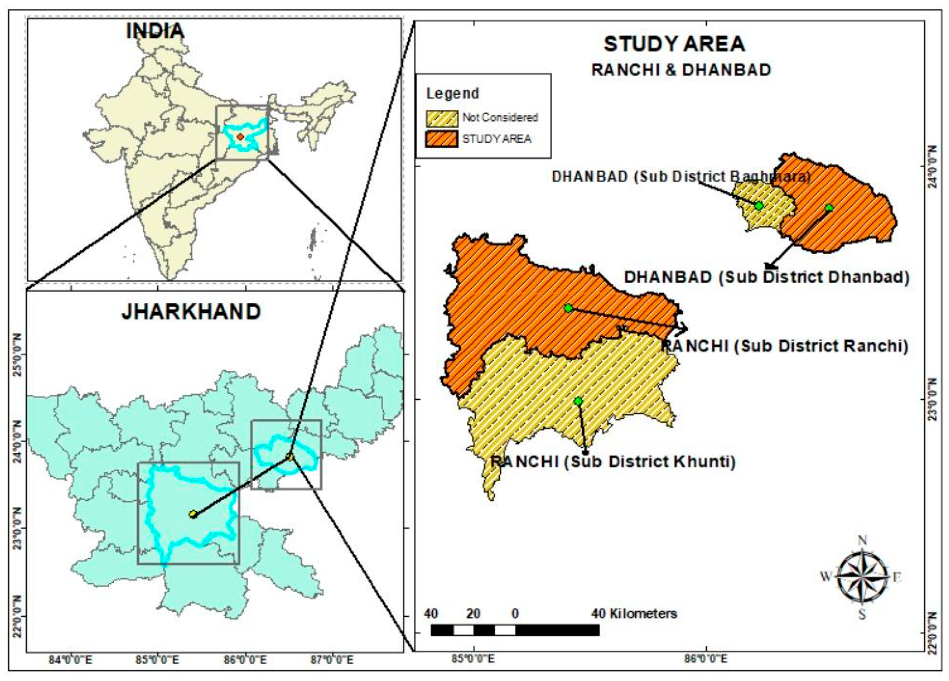
3. Study Area

In recent decades, Jharkhand state has experienced swift urbanization and exponential migration resulting in a significant population increase, leading to distinct LULC changes, particularly in the periphery of major developing cities and districts. The development of contemporary industry, particularly around the state and industrial capital, has accelerated urbanization. Ranchi and Dhanbad districts (Figure 1) have experienced significant changes in LULC, leading to many environmental problems. These changes may be linked to population expansion, altered farming techniques [77], and the implementation of numerous development projects over the previous two decades.

Dhanbad and Ranchi are 152 km apart, come under the Chota Nagpur plateau, and are famous minerals like Mica, Coal, Bauxite, lime, etc. To understand the dynamics of the built environment and the impact of LULC on radiated temperature, a spatial-temporal analysis of two major urban agglomerations (Ranchi and Dhanbad) was carried out. According to the 2011 Census, Ranchi and Dhanbad collectively accommodate a population of roughly 5 million individuals, with Ranchi being the more populous. Ranchi, the capital of Jharkhand state, has undergone significant urbanization owing to its economic and demographic expansion. The district encompasses an area of 5097 km² and is inhabited by 291,425 individuals. Ranchi is situated at the southernmost extremity of the Chota Nagpur plateau, which functions as the eastern frontier of the Deccan plateau.

The average elevation of Dhanbad and Ranchi is 222 m and 645 m, respectively. While Dhanbad geographical coordinates are 23.7957° N to 86.4304° E, Ranchi’s are 23°22′ N to 85°20′ E [77]. Moreover, while Dhanbad experiences a somewhat tropical wet and dry climate with summer and winter temperatures varying from 24–44.5 °C to 8–25 °C, Ranchi has a subtropical climate with a monsoon effect, i.e., 20–42 °C in summers and 2–25 °C in winters [77,78]. Relative humidity in Dhanbad and Ranchi fluctuates between 100% to 20% and 80% to 40% during monsoon and summer. Furthermore, Dhanbad and Ranchi experience an average yearly rainfall of 1598 mm and 1430 mm, respectively [77]. The principal rivers across the districts are Damodar and Subernarekha [14].

The present study considers ‘Sub District Ranchi’, which includes 14 blocks, as illustrated in Figure 2, for its LST analysis. Dhanbad is also known as the coal capital of Jharkhand due to the abundant availability of the coal mining industry and has the second-highest population after Ranchi [79,80]. According to (Census 2011), the people of the Dhanbad district is 1,560,384, covering an area of 2074.68 km². Dhanbad district is also divided into two sub-districts. While the former consists of two blocks, Baghmara and Topchanchi, the latter includes Gobindpur, Tundi, PurbTundi, Balliapur, Nirsa, Sindri, and Dhanbad Central. In our analysis, Dhanbad (Sub District Dhanbad) has been considered, including seven blocks as illustrated in Figure 2a, for its radiated temperature analysis.

Table 1. Geographical information related to the study area.

Parameter	Dhanbad	Ranchi
Latitude	23.7957° N	23.3441° N
Longitude	86.4304° E	85.3096° E
Population	1,560,384	291,425
Area (sq. km)	2074.68	5097
Climate	Humid sub-tropical	Moist sub-humid
Elevation (m)	222	651
Average Rainfall (mm)	1598	1355

highlights the physiographic features of the study areas.

4. Materials and Methods

The present study involves the calculation of LST using standard formulae available on the USGS webpage, which includes the stepwise calculation of parameters (BT, NDVI, Emissivity, etc.) discussed in detail in the procedure section below. Figure 3 attempts to provide a visual representation of the methodology of the research work.

4.1. Datasets

The Landsat-8 Operational Land Imager (OLI) data were utilized to assess and classify LST. The Landsat-8 has captured thermal images of the Earth’s surface using its recently launched TIRS sensors, which offer high-resolution capabilities. The satellite imagery in .tiff format was retained from United States Geological Survey (USGS) Earth Explorer, an open-access resource. The data contained within the portal has been gathered at regular 16-day intervals and has a resolution of 30 m and WGS1984 coordinate systems. The Landsat-8 OLI satellite data, belonging to the Landsat series of the National Aeronautics and Space Administration (NASA), has been noted by [82] for its 12-bit dynamic range The characteristic as mentioned earlier is accountable for enhancing the precision of radiation and the ratio of signal strength to background noise. Enhancement of land cover characteristics can be achieved through the improvement of the signal-to-noise ratio.

Table 2. LANDSAT-8_OLI and TIRS.

Band	Wavelength (Micrometers)	Resolution (Meters)	Band	Wavelength (Micrometers)	Resolution (Meters)
Band 1—Ultra Blue (coastal/aerosol)	0.435–0.451	30	Band 6—Shortwave Infrared (SWIR) 1	1.566–1.651	30
Red	0.452–0.512	30	Band 7—Shortwave Infrared (SWIR) 2	2.107–2.294	30
Band 3—Green	0.533–0.590	30	Band 8—Panchromatic	0.503–0.676	15
Band 4—Red	0.636–0.673	30	Band 9—Cirrus	1.363–1.384	30
Band 5—Near Infrared (NIR)	0.851–0.879	30	Band 10—Thermal Infrared (TIRS) 1	10.60–11.90	30
			Band 11—Thermal Infrared (TIRS) 2	11.50–12.51	30

summarizes the bandwidth specifications, including wavelength, electromagnetic spectrum, and resolution in meters.

The study also includes estimation brightness temperature Band 10 (TIRS1) was used, and for the NDVI generation of the study, area bands 4 and 5 were analyzed. Band 10 is recommended by USGS and is utilized alongside band 11 for the calculations even because of the inconsistencies in band 11. The classification of land use is facilitated through the utilization of Bands 4, 5, 6, and 7, while the calculation of indices is based on land cover. The study did not utilize certain spectral bands such as the Coastal Aerosol (band 1), Panchromatic (band 8), or Cirrus (Band 11).

Satellite imagery of dates (17 March 2019, 4 April 2020, 7 April 2021, and 17 April 2022) was considered for Ranchi and Dhanbad to effectively analyze LST in the study area. For image processing, image correction, area of interest cutting, preparing the vegetation index, and estimate of LST, among other tasks, ArcGIS 10.8 was employed. Images obtained are free from cloud cover and further corrected for additional atmospheric disturbances. The bands’ metadata from Landsat 8 were utilized to calculate LST. Images were reclassified using the closest neighbor method, and all data was re-projected onto the datum WGS84, zone 43, Universal Transverse Mercator (UTM) coordinate system. The atmospheric corrections are carried out in this investigation using an established based on image dark object removal model, as suggested by [83].

Table 3. Meta Data.

YEAR	District	Radiance Add Band	Radiance Mult Band	K1 Constant Band-10	K2 Constant Band-10
2019–2022	Ranchi	0.10000	0.0003342	774.8853	1321.0789
	Dhanbad	0.10000	0.0003342	774.8853	1321.0789

represents metadata used to calculate parameters (BT, PV, Emissivity, and LST). The subsequent paragraphs provide details on the datasets, the methodology employed for data processing, and the statistical techniques utilized for detecting discrepancies in diverse spectral values.

4.1.1. Estimation of Top of Atmosphere (TOA) Spectral Radiance

In order to improve the accuracy of satellite data products, geometric corrections were made. For the first part of the study, the formula and equation for L, or thermal spectral radiance (Watt/(m² × sr × nm)) is used to rescale the band 10 DN (Digital Number) data to at sensor spectral radiance [84] is as follows:

(L_Λ) = M_L × Q_cal + A_L

(1)

where A_L is the additive rescaling factor, i.e., radiance number of add band, M_L is the Multiplicative rescaling factor (radiance band number), and Q_cal (Quantized and Calibrated Standard Product Pixel) is the DN value of the picture and its corresponding band [85].

4.1.2. TOA to BT Transformation

The brightness temperature (BT) is determined by ground thermal radiance and is computed at the satellite level. By converting the DN values into sensor spectral radiance (BT), we calculated the brightness temperature for the TIRS band data. The TIRS band data was converted from spectral radiance to BT using thermal constants provided in the metadata file.

$$\mathrm{BT}=\frac{K2}{ln(\frac{K1}{L\lambda }+1)}-273.5$$

(2)

where K2 and K1 (thermal conversion constant) of the thermal infrared band (K) defines BT, while) Moreover, $L\lambda$ is spectral radiance. Moreover, to further convert the radiant temperature to degrees Celsius, an addition of 273.15 °C (making absolute zero) [85].

4.1.3. Determining the NDVI

The Normalized Difference Vegetation Index (NDVI) is a vegetation index that has been normalized and calculated based on the near-infrared (Band5) and surface-reflectance of red bands (Band4) [82]. It is significant to calculate NDVI to estimate the Pv (Proportion of Vegetation), which is essential for calculating emissivity (ε), without which calculation of LST is impossible. NDVI was determined using the formula [85] below;

$$NDVI=\frac{\left(Band 5 - Band 4\right)}{(Band 5+Band 4)},$$

(3)

4.1.4. Pv Estimation

Proportional vegetation (Pv) was determined from NDVI values obtained in step 4. This parameter approximates the extent of various land uses or land covers [86]

$$Pv={\left(\frac{NDVI-NDVI min}{\left(NDVI max-NDVI min\right)}\right)}^2,$$

(4)

where Vegetation proportion (Pv) is directly proportional to the square of the ratio of the difference between the calculated DN value and its minimum value of NDVI image to the difference of DN maximum and minimum value from NDVI images [85].

4.1.5. Land Surface Emissivity (ε) Determination

Based on NDVI, land surface emissivity (LSE) measures the average emissivity of a surface area on Earth. The computation of LST necessitates the computation of LSE. Emissivity is calculated by calibrating the vegetation proportion [85].

ε = 0.004 × Pv + 0.986,

(5)

4.1.6. Land Surface Temperature Estimation

The radiation wavelength, LSE, and the top-of-atmosphere brightness temperature were measured in the LST [87]. Notably, the Local Standard Time is not equivalent to the atmospheric temperature. The following equation was used to compute $Local Standard Time$ in (°C);

$$\mathrm{L}\mathrm{a}\mathrm{n}\mathrm{d} \mathrm{S}\mathrm{u}\mathrm{r}\mathrm{f}\mathrm{a}\mathrm{c}\mathrm{e} \mathrm{T}\mathrm{e}\mathrm{m}\mathrm{p}\mathrm{e}\mathrm{r}\mathrm{a}\mathrm{t}\mathrm{u}\mathrm{r}\mathrm{e}=\left(\frac{BT}{1}\right)+\lambda \times \left(\frac{BT}{\mathrm{14,380}}\right)\times Ln \left(\epsilon \right)$$

(6)

where $\lambda$ = wavelength of emitted radiance, BT = atmosphere brightness temperature, and Ln ($\epsilon$) is the logarithmic function of thermal emissivity (adimensional) [85,87].

4.1.7. Kriging Interpolation

The study incorporated the kriging interpolation method for investigating and depicting the unbiassed predicted values of LST. Kriging, a geostatistical approach derived from statistics, can be described as a process consisting of two steps. Firstly, estimating a variogram or semivariogram characterizes the spatial relationship between the sampled points. Semi variogram provides information through a visual depiction of the covariance between each pair of points in the sampled structure data. In the second step, weights derived from the estimated covariance structure are employed to estimate values for unsampled points or blocks over continuous spatial surfaces using a limited set of sample data points within the spatial domain. It is ideal for estimating the uncertainty surrounding each interpolated value (points). Moreover, Kriging is an optimal linear predictor and interpolator, i.e., each interpolated value is calculated to minimize the prediction error for that point. It is beneficial when there is a spatially associated distance or directional bias in the sampled data, which was also present in our data due to the sophisticated surface construction of the study area.

The approach was used to interpolate collected data and provide a concise picture of our data sets. Kriging weighted linear combination of the known sample values surrounding the point was calculated because Kriging considers both the distance between available data points and the degree of variability when estimating values for unknown regions, i.e., points closer to the location of interest are given more weightage than those farther away. Furthermore, Kriging invalidates the effect of clustered points by weighing them less heavily, thereby reducing the biases in prediction.

Therefore, raster points were firstly allocated raster values using the ArcGIS Database Management tool. While the ordinary kriging model was chosen as the semivariogram properties, the software suggested the best-fitting variogram model (spherical) along with the search radius. The process yields a surface approximation based on a distribution of points with z-values. Kriging Interpolation in ArcGIS resulted in sample sites’ spatial separation and orientation. In contrast, the spatial correlation was utilized to elucidate the alterations in LST within the designated area of interest.

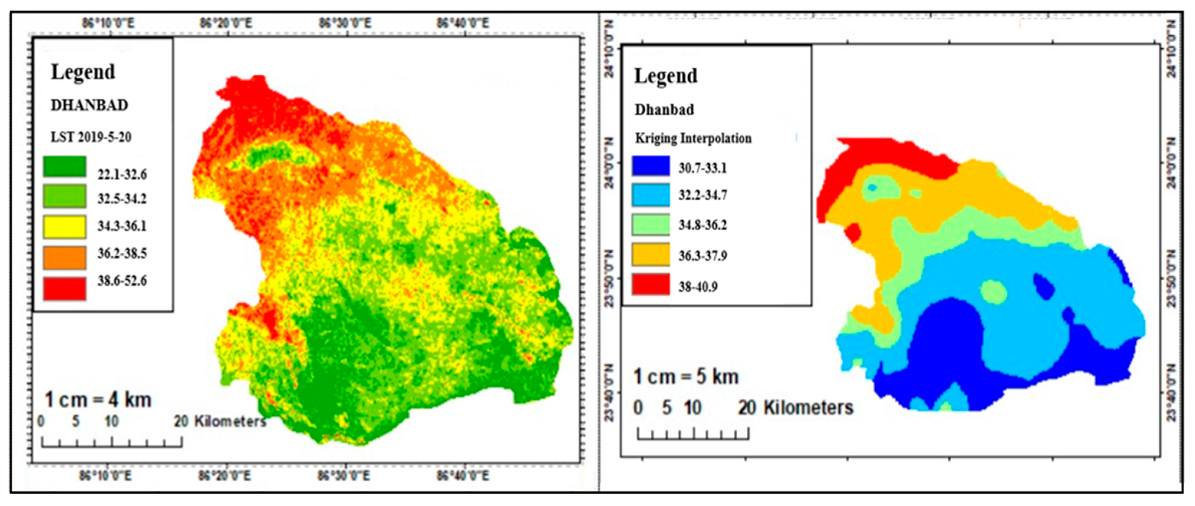
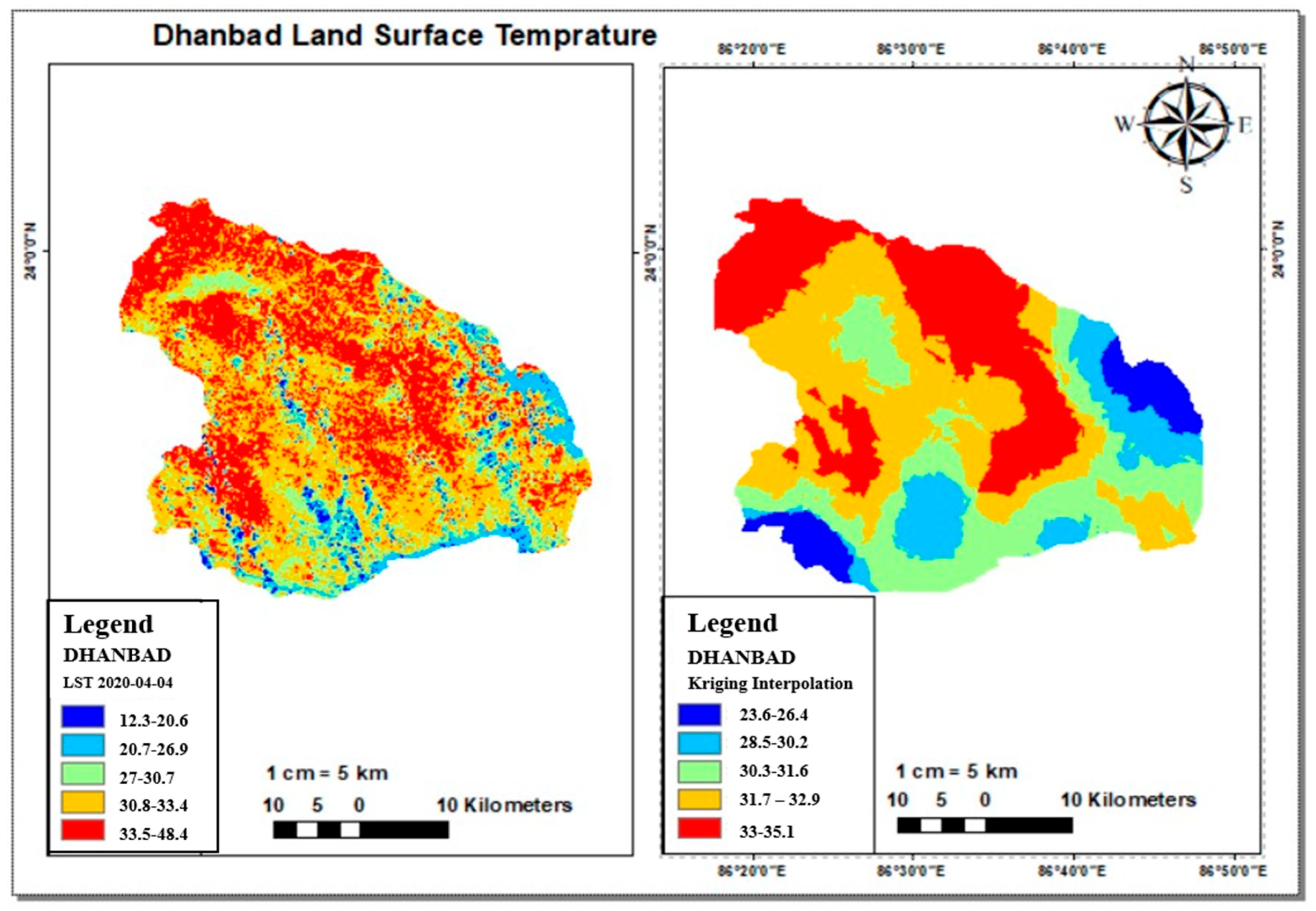
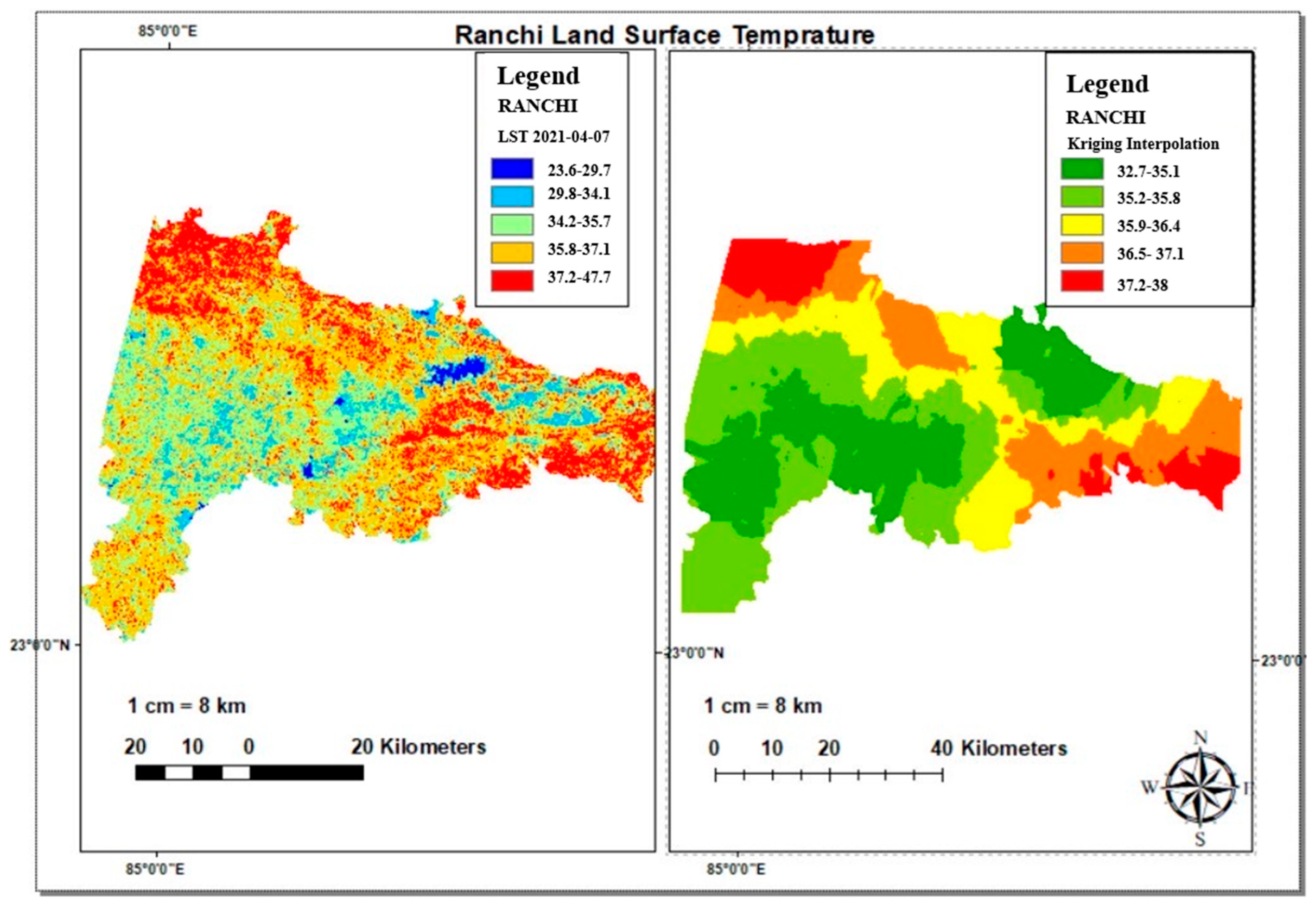
5. Results and Discussion

Gupta et al. (2020) [26] assessment of vegetation quantity through the detection of the contrast between near-infrared light, which is reflected intensely by vegetation, and red light is carried out by the NDVI. (Which vegetation absorbs). According to Kumar and Kumar (2020) [87], it can be observed that the human eye perceives green as vegetation. The NDVI exhibits a range of negative and positive values within a given boundary region. While the negative value highlights less or no vegetation or water availability, the NDVI value corresponding to +1 represents a high possibility of dense vegetation (green forest or agricultural lands) [26]. However, the NDVI value close to zero indicated the presence of an urbanized area. In our analysis, Landsat was considered the satellite sensor with the band, i.e., NIR and RED. A high NDVI value will result from a solution produced by the NDVI formula having less reflectance (low value) in the red channel, greater reflectance in the NIR channel, and vice versa.

Figure 4a,b depicts the NDVI of Ranchi and Dhanbad for 2019 and 2022. This is mainly illustrated to indicate the decrease in vegetation with a simultaneous increase in concrete settlements between the period in the districts. For Ranchi NDVI value ranged from −0.224 to 0.559 in 2019, and in 2022 this changed to −0.193 to 0.517 (Figure 4a), depicting that not only has there been decrement in vegetation and greener land cover but also a subsequent decrease of available surface water has been experiencing by the district’s populace. Similarly, in Dhanbad, as illustrated in Figure 4b, the NDVI ranged from −0.111 to 0.506 in 2019. It decreased from −0.109 to 0.462 in 2022, indicating the rapid depletion of vegetation in the area, making it a cause of concern.

ε (emissivity) is a critical surface parameter and an intrinsic property of all matter, which can be derived from measured emitted radiative emissions from space. Along with the surface temperature, wavelength and angle impact the calculated emissivity. The study utilized the NDVI threshold approach method to create LSE. As illustrated in Figure 5a,b, LSE was higher in the southern, south-eastern, and western districts because these areas were substantially elevated and had greater vegetative cover than the northern and central portions of the investigated area. The LSE of the Ranchi district ranged between 0.986–0.987 (in 2019) and varied between 0.98 and 0.99 (in 2022), as shown in Figure 5a. This was also evident in Dhanbad, where emissivity ranged from 0.986 to 0.989 (Figure 5b) over 4 years.

The average mean temperature ranged from 32.8 to 40.9 degree Celsius (Figure 6a) in Ranchi. In contrast, in Dhanbad, the temperature varied from 31.5 to 39.7 °C (Figure 6b), both having the lowest temperature during the lockdown in 2020. For all years under consideration, it was evident that Ranchi’s temperature remained at a minimum of 1 °C and higher than in Dhanbad. Figure 6a depicts the mean temperature variation of LST and its Kriging Interpolation in Ranchi and Dhanbad, where the solid line represents the linear trendline of LST and the dotted line depicts the moving average trend variations. The most difference of almost 4 °C was observed in 2019 between the two districts just 4 h apart. This observation was contrary to the author’s hypothesis that Dhanbad, the coal hub of Jharkhand, shall experience a rather hotter climate. However, the analysis shows that the capital district remained hotter in the dry months between 2019 and 2022.

The study utilized the LST derived from top atmosphere BT, emissivity, and emitted radiance wavelength to examine the temperature fluctuations over 4 years. The selection of Landsat data dates was based on the criterion that the period should exhibit minimal cloud and scene land cover, specifically less than 10%. Furthermore, data collection was restricted to the dry months of March, April, and May, during which a relatively dry atmosphere prevailed in the chosen study region. The range of water vapor values was comparatively low. Consequently, the attained outcomes did not necessitate atmospheric correction, and its impact was not factored in the LST computation.

The result from the experimental analysis depicted a significant decrease in temperature in degree Celsius experienced during the early months of 2020 compared to its preceding and succeeding years, i.e., 2019 & 2021, for both the study area, as illustrated in Figure 6a,b. This decrease can be attributed to the pre-existing lockdown and unlock-down process (

Table 4. COVID-19 Lockdown & Unlock-down Timeline.

Lockdown in 2020-1st Wave	Unlock 2020-1st Wave
Phase 1 (24 Mr *–14 A *)	Phase 1 (1–30 J *)
Phase 2 (15 A *–3 M *)	Phase 2 (1–31 Jy *)
Phase 3 (4–17 M *)	Phase 3 (1–31 Au *)
Phase 4 (18–31 M *)	Phase 4 (1–30 S *)
	Phase 5 (1–31 O *)
	Phase 6 (1–30 N *)
Lockdown in 2021-2nd Wave
April 5–June 15

* (Mr = March, A = April, M = May, J = June, Jy = July, Au = August, S = September, O = October, and N = November).

), which occurred in 2020 when the first wave of COVID-19 struck, forcing many carbons and other greenhouse gases emitting industries to remain closed. The lockdown distinctly restricted pollution-emitting sectors, including the transportation sector, which directly impacted the overall temperature of India. In this case, our study area also showed the same consistency.

Figure 7, Figure 8, Figure 9, Figure 10, Figure 11, Figure 12, Figure 13 and Figure 14 highlight the spatial distribution maps for LST during 2019-2022 in Ranchi and Dhanbad. The findings showed that the northeastern and eastern parts, including blocks like Ormanjhi, Rahe, Silli, and Angara, were much cooler than their western counterparts (Figure 7, Figure 9, Figure 11 and Figure 13). This can be attributed to its more extensive vegetation cover, which can be observed from the illustration of NDVI Figure 5. The blocks of Lapung, Kanke, Mander, and Khilari were comparatively hotter in all years. The same trend was seen in the Dhanbad district, where southern and south-eastern regions were much cooler; northern parts remained hottest. Southern blocks of Nirsa, Ballapur, Sindri, and parts of Dhanbad central experienced temperature variation of 26–32 °C in 2019 and 2020 (Figure 8, Figure 9 and Figure 10), but it drastically increased in 2021–2022 (Figure 12, Figure 13 and Figure 14). Moreover, Tundi and northern Gobindpur, where most of the coal sites of Dhanbad are located, remained hot for all four years. Figure 8, Figure 10, Figure 12 and Figure 14 indicate a direct interlinking and influence of coal mining on the region’s temperature. Moreover, it is notable that the higher vegetative cover was more apparent in high altitude areas (hilly terrains), as depicted in Figure 15, in both regions under focus and simultaneously experienced reduced exposure to higher LST variations.

Human interference is considered one of the most significant environmental challenges worldwide. It is essential to understand the changes related to area-specific characteristics and man–environment interactions because of their distinct impact on the regional landscape and disrupts the energy balance [88]. Study of GHG NO₂, CO, and PM10 concentration, which are predominant contributors to climate change and have been linked to various health issues [89] in such an exceptional opportunity—the COVID-19 Lockdown—is crucial and necessary to study, understand and assist public agencies and urban planners into adopting pollution reduction strategies, which shall contribute in map creation of urban areas that are robust and resistant to climate change in terms of SUHI and LST phenomenon. Indian urban hotspots facing migration and an urban agglomeration over the past three decades are negatively affected by the consequences of unplanned development [23]. As such, an attempt to map LULC traits to analyze urban expansion and evaluate the effects of anthropogenic activity on the environment is made in this study. Such research helps generate substantial knowledge about LST when the world is feeling the effects of the climate crisis and establishes a relationship between LST and other climatic geospatial metrics. This knowledge could further be used to develop strategies for reducing the climate phenomenon in emerging nations.

6. Conclusions

By estimating LST using ArcGIS and its existing equations, the research highlights the relationship between human activities and the actual impact of the COVID-19 closure on the urban surface temperature. This research is significant as it contributes to understanding how human activities, such as urbanization and land use changes, affect the local microclimate of the surrounding. It also provides insights into the potential for mitigating the UHI effect and encourages the formulation of sustainable urban planning and climate change predictive and model mitigation strategies. The study efficiently determined radiated temperature and LST for the most populated district of Jharkhand (Ranchi &Dhanbad) for 2019, 2020, 2021, and 2022 to analyze the temperature variance during the driest months (April–May). The LST was accurately computed using existing LANDSAT-8 equations and parameters obtained from the thermal infrared bands (OLI and TIR).form the USGSplatform. Additionally, ArcGIS 10.8 remote sensing software was utilized to assess the study area’s NDVI, LSE, LST, and brightness temperature. The observations from the results of the study can be summarized as follows;

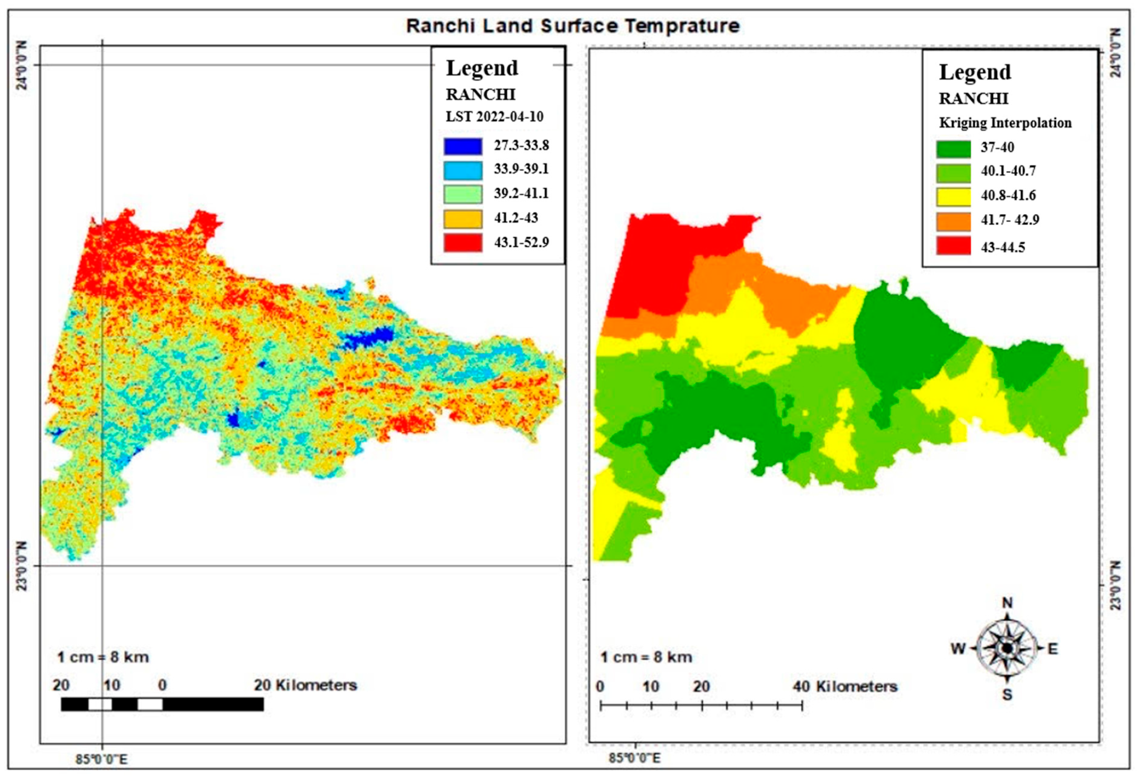
• The NDVI results from maps depict that vegetation cover is much more in the northeastern regions of Ranch and Dhanbad, which receive abundant rainfall and have lower concrete settlement penetration.
• Study results depicted that vegetative cover is higher in hilly areas in both districts, and with increases in elevation, LST decreased proportionately in the study area.
• Moreover, the LST in the southern & south-eastern parts was low in Dhanbad, while it was evident in the northeastern plateaus of Ranchi.
• The uncultivable lands of (Khilgir and/or Tundi) plains with barren lands in both study areas had higher urban penetration, which experienced comparatively high LST.
• The year of COVID-19, i.e., 2020, reported the lowest temperature in Ranchi & Dhanbad.
• The capital Ranchi remained a minimum of 1 degree Celsius hotter than Dhanbad even in 2020.
• The study also highlights that although both districts in 2019 experienced harsh summer temperatures of more than 40 °C temperature across various regions, it is 2022 which has become the hottest year, with summer temperatures reaching as much as 44.5 °C in the urban centers, depicting the impact of reduced man-incurred activity has faded away and the regions after confronting two consecutive comfortable summers the citizens are now vulnerable to sweltering heat.
• By comparing LST during the lockdown period with the pre-pandemic period, we observed a significant drop in temperature, indicating a meaningful relationship between human activities and urban surface temperature. This analysis provides insights into the impact of reduced human activities during the lockdown on the urban thermal environment and highlights the potential influence of anthropogenic heat on urban temperature.

Furthermore, the results revealed that cool airflow might be obtained in city centers if a belt of undeveloped and ideally vegetated land is provided around the metropolis. Our research highlights the possibility of future research on delineating heat islands for large urban areas using a similar methodology, as applied to UHI, seismic movement, thermal springs, stubble burning volcanic, coal mines, forest fires, and their impact on temperature variations.

References

- Sajjad, S.H.; Khan, T.; Qadri, S.M.T.; Gilani, N.; Waheed, S. Natural Hazards and Related Contents in Curriculum of Geography in Pakistan. Asian J. Nat. Appl. Sci. 2014, 3, 40–48. [Google Scholar]
- Rahman, Z.; Rehman, K.; Ali, W.; Ali, A.; Burton, P.; Barkat, A.; Ali, A.; Qadri, S.M.T. Re-Appraisal of Earthquake Catalog in the Pamir—Hindu Kush Region, Emphasizing the Early and Modern Instrumental Earthquake Events. J. Seism. 2021, 25, 1461–1481. [Google Scholar] [CrossRef]
- Qadri, S.M.T.; Mirza, M.Q.; Raja, A.; Yaghmaei-Sabegh, S.; Hakimi, M.H.; Ali, S.H.; Khan, M.Y. Application of Probabilistic Seismic Hazard Assessment to Understand the Earthquake Hazard in Attock City, Pakistan: A Step towards Linking Hazards and Sustainability. Sustainability 2023, 15, 1023. [Google Scholar] [CrossRef]
- Talha Qadri, S.M.; Nawaz, B.; Sajjad, S.H.; Sheikh, R.A. Ambient Noise H/V Spectral Ratio in Site Effects Estimation in Fateh Jang Area, Pakistan. Earthq. Sci. 2015, 28, 87–95. [Google Scholar] [CrossRef]
- Qadri, S.M.T.; Sajjad, S.H.; Sheikh, R.A.; Rehman, K.; Rafi, Z.; Nawaz, B.; Haider, W. Ambient Noise Measurements in Rawalpindi—Islamabad, Twin Cities of Pakistan: A Step towards Site Response Analysis to Mitigate Impact of Natural Hazard. Nat. Hazards 2015, 78, 1111–1123. [Google Scholar] [CrossRef]
- Talha Qadri, S.M.; Aminul Islam, M.; Shalaby, M.R.; Khattak, K.R.; Sajjad, S.H. Characterizing Site Response in the Attock Basin, Pakistan, Using Microtremor Measurement Analysis. Arab. J. Geosci. 2017, 10, 267. [Google Scholar] [CrossRef]
- Qadri, S.M.T.; Malik, O.A. Establishing Site Response-Based Micro-Zonation by Applying Machine Learning Techniques on Ambient Noise Data: A Case Study from Northern Potwar Region, Pakistan. Environ. Earth Sci. 2021, 80, 53. [Google Scholar] [CrossRef]
- Talha Qadri, S.M.; Shah, A.A.; Sahari, S.; Raja, A.; Yaghmaei-Sabegh, S.; Khan, M.Y. Tectonic Geomorphology-Based Modeling Reveals Dominance of Transpression in Taxila and the Contiguous Region in Pakistan: Implications for Seismic Hazards. Model. Earth Syst. Environ. 2023, 9, 1029–1050. [Google Scholar] [CrossRef]
- Shah, A.A.; Qadri, T.; Khwaja, S. Living with Earthquake Hazards in South and South East Asia. ASEAN J. Community Engag. 2018, 2, 15. [Google Scholar] [CrossRef]
- Khan, M.Y.; Turab, S.A.; Ali, L.; Shah, M.T.; Qadri, S.M.T.; Latif, K.; Kanli, A.I.; Akhter, M.G. The Dynamic Response of Coseismic Liquefaction-Induced Ruptures Associated with the 2019 Mw 5.8 Mirpur, Pakistan, Earthquake Using HVSR Measurements. Lead. Edge 2021, 40, 590–600. [Google Scholar] [CrossRef]
- United Nations. 68% of the World Population Projected to Live in Urban Areas by 2050, Says UN, UN DESA, United Nations Department of Economic and Social Affairs. Available online: https://www.un.org/development/desa/en/news/population/2018-revision-of-world-urbanization-prospects.html (accessed on 1 July 2023).
- Mallik, R.; Dikkila Bhutia, K.; Roy, S.; Nandi, M.; Dash, P.; Mukherjee, K. Spatio-Temporal Analysis of Environmental Criticality: Planned Versus Unplanned Urbanization. IOP Conf. Ser. Earth Environ. Sci. 2023, 1164, 012014. [Google Scholar] [CrossRef]
- Jardas, M.; Perić Hadžić, A.; Tijan, E. Defining and Measuring the Relevance of Criteria for the Evaluation of the Inflow of Goods in City Centers. Logistics 2021, 5, 44. [Google Scholar] [CrossRef]
- Sahana, M.; Dutta, S.; Sajjad, H. Assessing Land Transformation and Its Relation with Land Surface Temperature in Mumbai City, India Using Geospatial Techniques. Int. J. Urban Sci. 2019, 23, 205–225. [Google Scholar] [CrossRef]
- Tiwari, A.; Suresh, M.; Jain, K.; Shoab, M.; Dixit, A.; Pandey, A. Urban landscape dynamics for quantifying the changing pattern of urbanisation in delhi. J. Rural Dev. 2018, 37, 399. [Google Scholar] [CrossRef]
- Kammen, D.M.; Sunter, D.A. City-Integrated Renewable Energy for Urban Sustainability. Science 2016, 352, 922–928. [Google Scholar] [CrossRef] [PubMed]
- Agergaard, J.; Tacoli, C.; Steel, G.; Ørtenblad, S.B. Revisiting Rural–Urban Transformations and Small Town Development in Sub-Saharan Africa. Eur. J. Dev. Res. 2019, 31, 2–11. [Google Scholar] [CrossRef]
- Kanos, D.; Heitzig, C. Figures of the Week: Africa’s Urbanization Dynamics. Available online: https://www.brookings.edu/articles/figures-of-the-week-africas-urbanization-dynamics/ (accessed on 1 July 2023).
- Seto, K.C.; Fragkias, M.; Güneralp, B.; Reilly, M.K. A Meta-Analysis of Global Urban Land Expansion. PLoS ONE 2011, 6, e23777. [Google Scholar] [CrossRef]
- Shi, K.; Cui, Y.; Liu, S.; Wu, Y. Global Urban Land Expansion Tends To Be Slope Climbing: A Remotely Sensed Nighttime Light Approach. Earths Future 2023, 11, e2022EF003384. [Google Scholar] [CrossRef]
- Alam, T.; Banerjee, A. Deciphering Urbanization and Spatial Disparity in South 24 Parganas District of West Bengal, India. In Proceedings of the 58th ISOCARP World Planning Congress; ISOCARP, Brussels, Belgium, 3–6 October 2022. [Google Scholar]
- Ketterer, C.; Matzarakis, A. Comparison of Different Methods for the Assessment of the Urban Heat Island in Stuttgart, Germany. Int. J. Biometeorol. 2015, 59, 1299–1309. [Google Scholar] [CrossRef]
- Shahfahad; Kumari, B.; Tayyab, M.; Ahmed, I.A.; Baig, M.R.I.; Khan, M.F.; Rahman, A. Longitudinal Study of Land Surface Temperature (LST) Using Mono- and Split-Window Algorithms and Its Relationship with NDVI and NDBI over Selected Metro Cities of India. Arab. J. Geosci. 2020, 13, 1040. [Google Scholar] [CrossRef]
- Parlow, E. Regarding Some Pitfalls in Urban Heat Island Studies Using Remote Sensing Technology. Remote Sens. 2021, 13, 3598. [Google Scholar] [CrossRef]
- Shafiq, M.U.; Rasool, R.; Ahmed, P.; Dimri, A.P. Temperature and Precipitation Trends in Kashmir Valley, North Western Himalayas. Theor. Appl. Clim. 2019, 135, 293–304. [Google Scholar] [CrossRef]
- Gupta, N.; Mathew, A.; Khandelwal, S. Spatio-Temporal Impact Assessment of Land Use / Land Cover (LU-LC) Change on Land Surface Temperatures over Jaipur City in India. Int. J. Urban Sustain. Dev. 2020, 12, 283–299. [Google Scholar] [CrossRef]
- Stewart, I.D.; Oke, T.R. Local Climate Zones for Urban Temperature Studies. Bull. Am. Meteorol. Soc. 2012, 93, 1879–1900. [Google Scholar] [CrossRef]
- Jallu, S.B.; Shaik, R.U.; Srivastav, R.; Pignatta, G. Assessing the Effect of COVID-19 Lockdown on Surface Urban Heat Island for Different Land Use /Cover Types Using Remote Sensing. Energy Nexus 2022, 5, 100056. [Google Scholar] [CrossRef]
- Guha, S.; Govil, S.; Diwan, P. Analytical Study of Seasonal Variability in Land Surface Temperature with Normalized Difference Vegetation Index, Normalized Difference Water Index, Normalized Difference Built-up Index, and Normalized Multiband Drought Index. J. Appl. Remote Sens. 2019, 13, 1. [Google Scholar] [CrossRef]
- Pathak, C.; Chandra, S.; Maurya, G.; Rathore, A.; Sarif, M.O.; Gupta, R.D. The Effects of Land Indices on Thermal State in Surface Urban Heat Island Formation: A Case Study on Agra City in India Using Remote Sensing Data (1992–2019). Earth Syst. Environ. 2021, 5, 135–154. [Google Scholar] [CrossRef]
- Degirmenci, K.; Desouza, K.C.; Fieuw, W.; Watson, R.T.; Yigitcanlar, T. Understanding Policy and Technology Responses in Mitigating Urban Heat Islands: A Literature Review and Directions for Future Research. Sustain. Cities Soc. 2021, 70, 102873. [Google Scholar] [CrossRef]
- Hao, X.; Li, W.; Deng, H. The Oasis Effect and Summer Temperature Rise in Arid Regions—Case Study in Tarim Basin. Sci. Rep. 2016, 6, 35418. [Google Scholar] [CrossRef] [PubMed]
- Fadhil, M.; Hamoodi, M.N.; Ziboon, A.R.T. Mitigating Urban Heat Island Effects in Urban Environments: Strategies and Tools. IOP Conf. Ser. Earth Environ. Sci. 2023, 1129, 012025. [Google Scholar] [CrossRef]
- Vuckovic, M.; Schmidt, J.; Ortner, T.; Cornel, D. Combining 2D and 3D Visualization with Visual Analytics in the Environmental Domain. Information 2021, 13, 7. [Google Scholar] [CrossRef]
- Arifwidodo, S.D.; Tanaka, T. The Characteristics of Urban Heat Island in Bangkok, Thailand. Procedia Soc. Behav. Sci. 2015, 195, 423–428. [Google Scholar] [CrossRef]
- Probst, N.; Bach, P.M.; Cook, L.M.; Maurer, M.; Leitão, J.P. Blue Green Systems for Urban Heat Mitigation: Mechanisms, Effectiveness and Research Directions. Blue Green Syst. 2022, 4, 348–376. [Google Scholar] [CrossRef]
- Hidalgo García, D.; Arco Díaz, J. Impacts of the COVID-19 Confinement on Air Quality, the Land Surface Temperature and the Urban Heat Island in Eight Cities of Andalusia (Spain). Remote Sens. Appl. Soc. Environ. 2022, 25, 100667. [Google Scholar] [CrossRef] [PubMed]
- Oke, T.R. Boundary Layer Climates; Routledge: Abingdon, UK, 2002; ISBN 0-203-40721-0. [Google Scholar]
- Fatemi, M.; Narangifard, M. Monitoring LULC Changes and Its Impact on the LST and NDVI in District 1 of Shiraz City. Arab. J. Geosci. 2019, 12, 127. [Google Scholar] [CrossRef]
- Rajeshwari, A. Estimation of land surface temperature of dindigul district using LANDSAT 8 data. Int. J. Res. Eng. Technol. 2014, 3, 122–126. [Google Scholar] [CrossRef]
- Mathew, A.; Sarwesh, P.; Khandelwal, S. Investigating the Contrast Diurnal Relationship of Land Surface Temperatures with Various Surface Parameters Represent Vegetation, Soil, Water, and Urbanization over Ahmedabad City in India. Energy Nexus 2022, 5, 100044. [Google Scholar] [CrossRef]
- Valjarević, A.; Djekić, T.; Stevanović, V.; Ivanović, R.; Jandziković, B. GIS Numerical and Remote Sensing Analyses of Forest Changes in the Toplica Region for the Period of 1953–2013. Appl. Geogr. 2018, 92, 131–139. [Google Scholar] [CrossRef]
- Tewari, A.; Srivastava, N. Impact of COVID Lockdowns on Spatio-Temporal Variability in Land Surface Temperature and Vegetation Index. Environ, Monit. Assess. 2023, 195, 507. [Google Scholar] [CrossRef]
- Chakraborty, T.; Sarangi, C.; Lee, X. Reduction in Human Activity Can Enhance the Urban Heat Island: Insights from the COVID-19 Lockdown. Environ. Res. Lett. 2021, 16, 054060. [Google Scholar] [CrossRef]
- Imhoff, M.L.; Zhang, P.; Wolfe, R.E.; Bounoua, L. Remote Sensing of the Urban Heat Island Effect across Biomes in the Continental USA. Remote Sens. Environ. 2010, 114, 504–513. [Google Scholar] [CrossRef]
- Teufel, B.; Sushama, L.; Poitras, V.; Dukhan, T.; Bélair, S.; Miranda-Moreno, L.; Sun, L.; Sasmito, A.P.; Bitsuamlak, G. Impact of COVID-19-Related Traffic Slowdown on Urban Heat Characteristics. Atmosphere 2021, 12, 243. [Google Scholar] [CrossRef]
- Akbari, H.; Konopacki, S. Calculating Energy-Saving Potentials of Heat-Island Reduction Strategies. Energy Policy 2005, 33, 721–756. [Google Scholar] [CrossRef]
- Chetia, S.; Saikia, A.; Basumatary, M.; Sahariah, D. When the Heat Is on: Urbanization and Land Surface Temperature in Guwahati, India. Acta Geophys. 2020, 68, 891–901. [Google Scholar] [CrossRef]
- Roshan, G.; Sarli, R.; Grab, S.W. The Case of Tehran’s Urban Heat Island, Iran: Impacts of Urban ’Lockdown’ Associated with the COVID-19 Pandemic. Sustain. Cities Soc. 2021, 75, 103263. [Google Scholar] [CrossRef]
- Arbuthnott, K.G.; Hajat, S. The Health Effects of Hotter Summers and Heat Waves in the Population of the United Kingdom: A Review of the Evidence. Environ. Health 2017, 16, 119. [Google Scholar] [CrossRef]
- Dwivedi, A.; Mohan, B.K. Impact of Green Roof on Micro Climate to Reduce Urban Heat Island. Remote Sens. Appl. Soc. Environ. 2018, 10, 56–69. [Google Scholar] [CrossRef]
- Macintyre, H.L.; Heaviside, C.; Taylor, J.; Picetti, R.; Symonds, P.; Cai, X.-M.; Vardoulakis, S. Assessing Urban Population Vulnerability and Environmental Risks across an Urban Area during Heatwaves—Implications for Health Protection. Sci. Total Environ. 2018, 610–611, 678–690. [Google Scholar] [CrossRef]
- Yang, C.; Yan, F.; Zhang, S. Comparison of Land Surface and Air Temperatures for Quantifying Summer and Winter Urban Heat Island in a Snow Climate City. J. Environ. Manag. 2020, 265, 110563. [Google Scholar] [CrossRef]
- Feizizadeh, B.; Blaschke, T. Examining Urban Heat Island Relations to Land Use and Air Pollution: Multiple Endmember Spectral Mixture Analysis for Thermal Remote Sensing. IEEE J. Sel. Top. Appl. Earth Obs. Remote Sens. 2013, 6, 1749–1756. [Google Scholar] [CrossRef]
- Santamouris, M. Recent Progress on Urban Overheating and Heat Island Research. Integrated Assessment of the Energy, Environmental, Vulnerability and Health Impact. Synergies with the Global Climate Change. Energy Build. 2020, 207, 109482. [Google Scholar] [CrossRef]
- Ghosh, P.; Baladandayuthapani, V.; Banerjee, M.; Mukherjee, B.; Ray, D. Predictions, Role of Interventions and Effects of a Historic National Lockdown in India’s Response to the the COVID-19 Pandemic: Data Science Call to Arms. Harv. Data Sci. Rev. 2020. [Google Scholar] [CrossRef] [PubMed]
- Hua, L.; Zhang, X.; Nie, Q.; Sun, F.; Tang, L. The Impacts of the Expansion of Urban Impervious Surfaces on Urban Heat Islands in a Coastal City in China. Sustainability 2020, 12, 475. [Google Scholar] [CrossRef]
- Huang, X.; Ding, A.; Gao, J.; Zheng, B.; Zhou, D.; Qi, X.; Tang, R.; Wang, J.; Ren, C.; Nie, W.; et al. Enhanced Secondary Pollution Offset Reduction of Primary Emissions during COVID-19 Lockdown in China. Natl. Sci. Rev. 2021, 8, nwaa137. [Google Scholar] [CrossRef]
- Arrofiqoh, E.N.; Setyaningrum, D.A. The Impact of COVID-19 Pandemic on Land Surface Temperature in Yogyakarta Urban Agglomeration. J. Appl. Geospat. Inf. 2021, 5, 480–485. [Google Scholar] [CrossRef]
- El Kenawy, A.M.; Lopez-Moreno, J.I.; McCabe, M.F.; Domínguez-Castro, F.; Peña-Angulo, D.; Gaber, I.M.; Alqasemi, A.S.; Al Kindi, K.M.; Al-Awadhi, T.; Hereher, M.E.; et al. The Impact of COVID-19 Lockdowns on Surface Urban Heat Island Changes and Air-Quality Improvements across 21 Major Cities in the Middle East. Environ. Pollut. 2021, 288, 117802. [Google Scholar] [CrossRef]
- Ali, G.; Abbas, S.; Qamer, F.M.; Wong, M.S.; Rasul, G.; Irteza, S.M.; Shahzad, N. Environmental Impacts of Shifts in Energy, Emissions, and Urban Heat Island during the COVID-19 Lockdown across Pakistan. J. Clean. Prod. 2021, 291, 125806. [Google Scholar] [CrossRef] [PubMed]
- Alqasemi, A.S.; Hereher, M.E.; Kaplan, G.; Al-Quraishi, A.M.F.; Saibi, H. Impact of COVID-19 Lockdown upon the Air Quality and Surface Urban Heat Island Intensity over the United Arab Emirates. Sci. Total Environ. 2021, 767, 144330. [Google Scholar] [CrossRef]
- Di Sabatino, S.; Barbano, F.; Brattich, E.; Pulvirenti, B. The Multiple-Scale Nature of Urban Heat Island and Its Footprint on Air Quality in Real Urban Environment. Atmosphere 2020, 11, 1186. [Google Scholar] [CrossRef]
- Schaefer, M.; Ebrahimi Salari, H.; Köckler, H.; Thinh, N.X. Assessing Local Heat Stress and Air Quality with the Use of Remote Sensing and Pedestrian Perception in Urban Microclimate Simulations. Sci. Total Environ. 2021, 794, 148709. [Google Scholar] [CrossRef]
- Avdan, U.; Jovanovska, G. Algorithm for Automated Mapping of Land Surface Temperature Using LANDSAT 8 Satellite Data. J. Sens. 2016, 2016, 1480307. [Google Scholar] [CrossRef]
- Srivastava, A.K.; Bhoyar, P.D.; Kanawade, V.P.; Devara, P.C.S.; Thomas, A.; Soni, V.K. Improved Air Quality during COVID-19 at an Urban Megacity over the Indo-Gangetic Basin: From Stringent to Relaxed Lockdown Phases. Urban Clim. 2021, 36, 100791. [Google Scholar] [CrossRef]
- Zambrano-Monserrate, M.A.; Ruano, M.A.; Sanchez-Alcalde, L. Indirect Effects of COVID-19 on the Environment. Sci. Total Environ. 2020, 728, 138813. [Google Scholar] [CrossRef] [PubMed]
- Das, N.; Sutradhar, S.; Ghosh, R.; Mondal, P. Asymmetric Nexus between Air Quality Index and Nationwide Lockdown for COVID-19 Pandemic in a Part of Kolkata Metropolitan, India. Urban Clim. 2021, 36, 100789. [Google Scholar] [CrossRef]
- Nakajima, K.; Takane, Y.; Kikegawa, Y.; Furuta, Y.; Takamatsu, H. Human Behaviour Change and Its Impact on Urban Climate: Restrictions with the G20 Osaka Summit and COVID-19 Outbreak. Urban Clim. 2021, 35, 100728. [Google Scholar] [CrossRef]
- Ban-Weiss, G.A.; Woods, J.; Millstein, D.; Levinson, R. Using Remote Sensing to Quantify Albedo of Roofs in Seven California Cities, Part 2: Results and Application to Climate Modeling. Sol. Energy 2015, 115, 791–805. [Google Scholar] [CrossRef]
- Potter, C.; Alexander, O. Impacts of the San Francisco Bay Area Shelter-in-Place during the COVID-19 Pandemic on Urban Heat Fluxes. Urban Clim. 2021, 37, 100828. [Google Scholar] [CrossRef]
- Mandal, I.; Pal, S. COVID-19 Pandemic Persuaded Lockdown Effects on Environment over Stone Quarrying and Crushing Areas. Sci. Total Environ. 2020, 732, 139281. [Google Scholar] [CrossRef]
- Fujibe, F. Temperature Anomaly in the Tokyo Metropolitan Area during the COVID-19 (Coronavirus) Self-Restraint Period. SOLA 2020, 16, 175–179. [Google Scholar] [CrossRef]
- He, G.; Pan, Y.; Tanaka, T. The Short-Term Impacts of COVID-19 Lockdown on Urban Air Pollution in China. Nat. Sustain. 2020, 3, 1005–1011. [Google Scholar] [CrossRef]
- Maithani, S.; Nautiyal, G.; Sharma, A. Investigating the Effect of Lockdown During COVID-19 on Land Surface Temperature: Study of Dehradun City, India. J. Indian Soc. Remote Sens. 2020, 48, 1297–1311. [Google Scholar] [CrossRef]
- Ali, S.S.; Kaur, R.; Gupta, H.; Ahmad, Z.; Elnaggar, G. Determinants of an Organization’s Readiness for Drone Technologies Adoption. IEEE Trans. Eng. Manag. 2021, 1–15. [Google Scholar] [CrossRef]
- Kumar, A.; Pandey, A.C.; Hoda, N.; Jeyaseelan, A.T. Evaluation of Urban Sprawl Pattern in the Tribal-Dominated Cities of Jharkhand State, India. Int. J. Remote Sens. 2011, 32, 7651–7675. [Google Scholar] [CrossRef]
- Mohanta, K.; Sharma, L.K. Assessing the Impacts of Urbanization on the Thermal Environment of Ranchi City (India) Using Geospatial Technology. Remote Sens. Appl. Soc. Environ. 2017, 8, 54–63. [Google Scholar] [CrossRef]
- Kumar, A.; Samadder, S.R. An Empirical Model for Prediction of Household Solid Waste Generation Rate—A Case Study of Dhanbad, India. Waste Manag. 2017, 68, 3–15. [Google Scholar] [CrossRef]
- Population Census 2011 India. Available online: https://www.census2011.co.in/ (accessed on 11 September 2022).
- Ranchi Tehsil Map. Available online: https://www.mapsofindia.com/maps/jharkhand/tehsil/ranchi.html (accessed on 17 December 2022).
- Yasir, M.; Hui, S.; Rahman, S.U.; Ilyas, M.; Zafar, A.; Mehmood, A. Estimation of Land Surface Temperature Using LANDSAT-8 Data—A Case Study of District Malakand, Khyber Pakhtunkhwa, Pakistan. J. Lib. Arts Humanit. 2020, 1, 10. [Google Scholar]
- Chavez, P.S. An Improved Dark-Object Subtraction Technique for Atmospheric Scattering Correction of Multispectral Data. Remote Sens. Environ. 1988, 24, 459–479. [Google Scholar] [CrossRef]
- Mohanasundaram, S.; Baghel, T.; Thakur, V.; Udmale, P.; Shrestha, S. Reconstructing NDVI and Land Surface Temperature for Cloud Cover Pixels of Landsat-8 Images for Assessing Vegetation Health Index in the Northeast Region of Thailand. Environ. Monit. Assess. 2023, 195, 211. [Google Scholar] [CrossRef]
- Cook, M.; Schott, J.; Mandel, J.; Raqueno, N. Development of an Operational Calibration Methodology for the Landsat Thermal Data Archive and Initial Testing of the Atmospheric Compensation Component of a Land Surface Temperature (LST) Product from the Archive. Remote Sens. 2014, 6, 11244–11266. [Google Scholar] [CrossRef]
- Rosado, R.M.G.; Guzmán, E.M.A.; Lopez, C.J.E.; Molina, W.M.; García, H.L.C.; Yedra, E.L. Mapping the LST (Land Surface Temperature) with Satellite Information and Software ArcGis. IOP Conf. Ser. Mater. Sci. Eng. 2020, 811, 012045. [Google Scholar] [CrossRef]
- Kumar, R.; Kumar, A. Estimation of Land Surface Temperature Using LANDSAT 8 Satellite Data of Panchkula District, Haryana. J. Geogr. Environ. Earth Sci. Int. 2020, 24, 47–66. [Google Scholar] [CrossRef]
- Bae, J.; Ryu, Y. Land Use and Land Cover Changes Explain Spatial and Temporal Variations of the Soil Organic Carbon Stocks in a Constructed Urban Park. Landsc. Urban Plan. 2015, 136, 57–67. [Google Scholar] [CrossRef]
- Bashir, M.F.; Ma, B.; Bilal; Komal, B.; Bashir, M.A.; Tan, D.; Bashir, M. Correlation between Climate Indicators and COVID-19 Pandemic in New York, USA. Sci. Total Environ. 2020, 728, 138835. [Google Scholar] [CrossRef] [PubMed]