Developing the Actual Precipitation Probability Distribution Based on the Complete Daily Series

Abstract

The defense against urban pluvial flooding relies on the prediction of rainfall frequency, intensity, and long-term trends. The influence of the choice of the complete time series or the wet-day series on the rain analyses remains unclear, which affects the adaptive strategies for the old industrial cities such as Changchun in Northeastern China, with the outdated combined sewer systems. Based on the data from the two separate weather stations, four types of distributions were compared for analyzing the complete daily precipitation series, and their fitting accuracy was found in decreasing order of Pearson III, Pareto–Burr–Feller distribution (PBF), generalized extreme value (GEV), and Weibull. The Pearson III and the PBF probability distribution functions established based on the complete time series were found to be at least 458% and 227%, respectively, more accurate in fitting with the consecutive observations than those built from the wet-day-only series, which did not take account of the probability of the dry periods between the rain events. The rain depths of the return periods determined from the wet-day-only series might be over-predicted by at least 76% if the complete daily series were regarded as being more closely representative of the real condition. A clear threshold of 137 days was found in this study to divide the persistent or autocorrelated time series from the antipersistent or independent time series based on the climacogram analysis, which provided a practical way for independence determination. Due to the significant difference in the rain analyses established from the two time series, this work argued that the complete daily series better represented the real condition and, therefore, should be used for the frequency analysis for flood planning and infrastructure designs.

1. Introduction

Pluvial flooding is a major type of natural disaster affecting urban development. The frequent occurrence of urban rain flood damage could cause serious losses of lives and properties such as the recent flooding event in Zhengzhou, Henan Province, China on 20 July 2021 [1]. In order to efficiently reduce the risk of urban waterlogging according to the current practices, it is reasonable to design the drainage system to cope with a series of rain events with a specified maximum recurrence, which could only be given by an accurate frequency analysis.

The widely used method for precipitation frequency analysis is fitting the observation data to a probability distribution curve intrinsically determined by the corresponding probability density function (PDF) that applies to a specific region. Pearson type III distribution was initially proposed for analyzing precipitation data in the early stage and was recommended as an ideal distribution [2], followed by Fréchet [3], Weibull [4], Gumbel [5], Burr [6] and generalized extreme value (GEV) distributions [7]. For small and ungauged basins, the continuity framework integrating the rain generator and the runoff models were usually applied [8,9], for which the parameter estimation played an important role in affecting the accuracy of the frequency analysis.

According to the increasing need for parameter estimation [10], the regional analysis method was widely used. As the main method of parameter estimation in the calibration of the regional analytical method, the L-moment method was proposed and quickly accepted due to its excellent unbiasedness and stability [11,12,13,14], and it can be a very good solution to the problem that the magnitudes of the large design storms are inaccurate [15,16], though the maximum likelihood method was found to better respond to the extreme values at the point scale [17]. But the regional methods have some limitations. First, regional analysis methods target the average condition of a region with a high demand for the number of stations and the duration of the data, which can be hardly met by a city without enough gauges and long-term observations. Second, through the literature survey, it was found that few studies have considered analyzing the rainfall frequency on a daily basis including dry days [18], but most studies rather considered the probability of rains only on rainy days, which tends to be a higher chance than the probability of rains without knowing in advance if a day will rain or not.

Historically, precipitation frequency analyses mainly used the incomplete time series of only wet days with non-zero rain data to fit the probability distributions, such as Gamma [19], Log-Pearson III [20], or the power-type distributions [21,22]. Recently, the generalized gamma distribution has been used to analyze rainfall data, providing insights into the link of the beta prime distribution [21,22].

Intuitively, the frequency analysis methods based on wet days instead of the complete time series do not accurately represent the daily rainfall probability, as they fail to consider the probability of rainfall occurrence. One disadvantage of using the wet-day rain series to build a probability distribution is that it assumes a rainy day as a prerequisite but does not convey the actual chance of a rain event on any given day. However, the actual chance of rainfall determines flood risk and hydraulic designs, and its distribution can be achieved by using a stochastic model that controls the occurrence of zeros. Only a few studies have explored the rain frequency from the complete daily series based on the log-normal [18,23] and the Pareto–Burr–Feller (PBF) distributions [24]. However, the difference in the performance of the models built on the complete versus the wet daily series is still unclear.

The persistence, or autocorrelation of the time series data was found to vary with the temporal scale [25,26]. The influence of incorporating a large sum of zero values into the rain series on the dependence structure of the time series becomes further complicated, but matters for the regional water supply and food security [27,28,29,30].

Meanwhile, developing the actual precipitation probability distributions also needs to consider the mutations in the long-term trend. In China, the rainfall has an overall increasing trend, while the rainfall of the northeastern part of China has increased by 119% above the multi-year average in 2020 [31,32].

Therefore, this work aims to use Changchun, Jilin Province, in Northeastern China as a case study to develop four types of actual precipitation probability distributions, and compared the accuracy of the models established by the complete daily series and by the wet-day series. The link between the long-term trend and the actual rainfall probability distributions was also investigated.

2. Methods

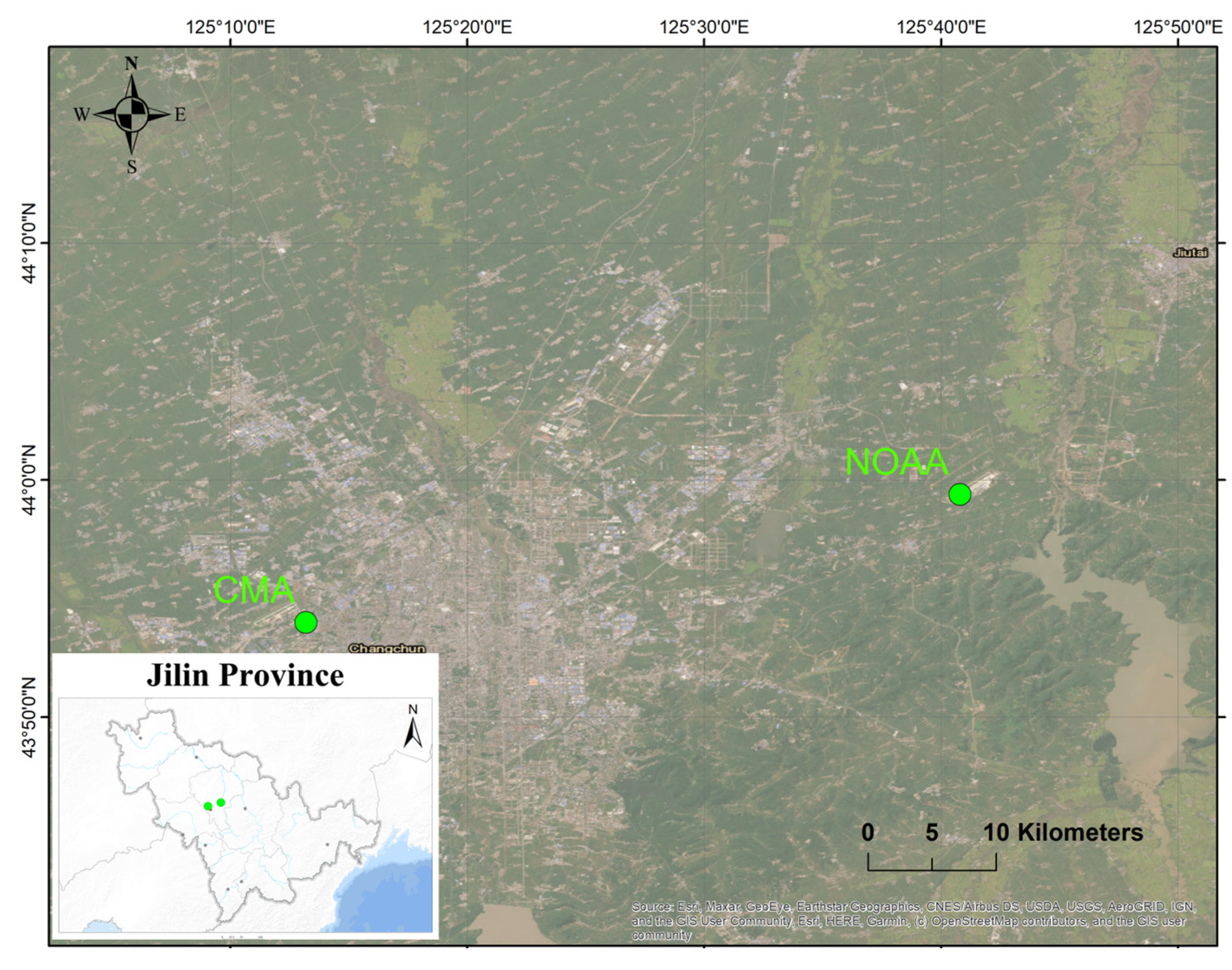
2.1. Data Preprocessing

This study collected the historic precipitation time series from the China Meteorological Administration (CMA; Station ID: 54161; Lat: 43.90° N; Lon: 125.22° E) and the National Oceanic and Atmospheric Administration (NOAA) of the United States (Station ID: 54161099999; Lat: 43.99° N; Lon: 125.68° E) (Figure 1). The CMA data were on a daily scale ranging from 1960 to 2019, while the NOAA data was on a 3 h scale ranging from 1960 to 2019 that were aggregated into daily values. The NOAA data had a ten-year missing gap from 1964 to 1973 (approximately 16% data loss), which was ignored by this study. The CMA station was close to the downtown with an annual precipitation of 584.68 mm, while the NOAA station was located in the northeastern region outside the city area with 591.19 mm yearly precipitation.

2.2. Probability Distributions

Four types of probability distributions were examined for the study area including Pearson type III, PBF, GEV, and Weibull. The probability density function of the Pearson type III distribution could be written as follows:

$$f(x)=\frac{{\beta }^a}{\Gamma \left(\alpha \right)}{\left(x-a_0\right)}^{\alpha -1}{e}^{-\beta \left(x-a_0\right)},$$

(1)

$$C_v=\frac{\sigma }{\overline{x}},$$

(2)

$$C_s=\frac{\sum {\left(x-\overline{x}\right)}^3}{\left(n-3\right){\sigma }^3},$$

(3)

$$a_0=\overline{x}\left(1-\frac{C_v}{C_s}\right),$$

(4)

where $f$ is the probability density of Pearson type III distribution, $\Gamma \left(\alpha \right)$ is the gamma function, α is the shape parameter, β is the scale parameters and $a_0$ is the location parameters, x is the sampled rainfall data. $\overline{x}$ is the mean of the sampled time series. $\sigma$ is the standard deviation of the sampled time series. These three parameters (α, β, and $a_0$) would determine the corresponding probability density function, and were estimated by the maximum likelihood method based on the skewness coefficient (C_s) and the variation coefficient (C_v) [33], e.g., the location parameter could be calculated by substituting (2) and (3) into Equation (4), as follows:

$$a_0=\overline{x}-\frac{\left(n-3\right){\sigma }^4}{\sum {\left(x-\overline{x}\right)}^3}.$$

(5)

The distribution function of the PBF distribution could be written as follows [24]:

$$F(x)=1-{\left(1+\left(\frac{x}{a}-h\right)\right)}^{-c},$$

(6)

where F(x) is the distribution function of PBF distribution, x represents the rainfall data, a is a dimensionless scale parameter, c is a dimensionless parameter characterizing the right tail (extreme events) of the distribution and h is a dimensionless parameter representing a threshold value and characterizing the left tail (dry events) of the distribution.

The probability density function of the GEV distribution could be written as follows [34]:

$$G(x)=exp\left(-{\left(1+\gamma \frac{x-\mu }{\sigma }\right)}^{-1/\gamma }\right),$$

(7)

where $G\left(x\right)$ is the probability function of GEV distribution, $\gamma$ is the shape parameter. In this distribution, when the parameter γ > 0, the distribution is an extreme type II distribution [35], $\sigma$ is the scale parameter, and $\mu$ is the position parameter. These three parameters were quantified through the maximum likelihood estimation as follows:

$$L(\theta )={\prod }_{i=1}^n p\left(x_i,p\right),$$

(8)

where L($\theta$) is the likelihood function, x_i is the rainfall data, $p$ is the parameter needed to estimate, and $p\left(x_i,\theta \right)$ is the univariate density function given a value of the dependent parameter.

The probability density function of the Weibull distribution could be written as follows [36]:

$$f(x)=\frac{\alpha (x-\theta {)}^{\alpha -1}}{\beta }exp\left(-{\left(\frac{x-\theta }{\beta }\right)}^{\alpha }\right),$$

(9)

where $f$ is the probability density of Weibull distribution density, α is the shape parameter, x is the rainfall data, β is the scale parameter, and θ is the position parameter.

It is worth noting that the GEV method requires consecutive records of the data series to be independent of each other [37]. But the Pearson type Ⅲ distribution does not have this requirement. To test the studied datasets, the serial correlation of the wet-day series and complete series could be calculated as follows:

$$r_1=\frac{\frac{1}{n-1}\sum _{i=1}^{n-1} \left(x_i-E\left(x_i\right)\right)\cdot \left(x_{i+1}-E\left(x_i\right)\right)}{\frac{1}{n}\sum _{i=1}^n {\left(x_i-E\left(x_i\right)\right)}^2},$$

(10)

$$E\left(x_i\right)=\frac{1}{n}{\sum }_{i=1}^n x_i,$$

(11)

where $r_1$ is the lag-1 serial correlation, $x_i$ is the rainfall data, $E\left(x_i\right)$ is the mean of sample data, and n is the sample size.

The serial correlation could be evaluated by following criterion [37]:

$$\frac{-1-1.645\sqrt{n-2}}{n-1}\le r_1\le \frac{-1+1.645\sqrt{n-2}}{n-1}.$$

(12)

The time series data would be considered serially correlated when $r_1$ value is outside the above interval; otherwise, the observations would be thought of as independent series.

The independence or the antipersistence of the time series can also be evaluated by the climacogram [38], as a double logarithmic plot of the standard deviation versus the averaging time scale k [39]. The standard deviation of a time scale k could be estimated by the classical law [40]:

$${\sigma }^{\left(k\right)}=\frac{\sigma }{\sqrt{k}},$$

(13)

where the ${\sigma }^{\left(k\right)}$ is the function of scale k. However, this law may not be applicable to natural systems, and the simplest alternative is [40]:

$${\sigma }^{\left(k\right)}=\frac{\sigma }{k^{1-H}},$$

(14)

where H is the Hurst coefficient (0 < H < 1) [41]. The slope of the double logarithmic plot is equal to H + 1. The time series could be regarded as antipersistent when the value of H falls into the range between 0 and 0.5 [40].

2.3. Skill Assessment

After the probability density models were established, their accuracy was evaluated based on Nash–Sutcliffe Efficiency (NSE):

$$\mathrm{N}\mathrm{S}\mathrm{E}=1-\frac{\sum _{i=1}^n {\left(q_i-p_i\right)}^2}{\sum _{i=1}^n {\left(q_i-\overline{q}\right)}^2},$$

(15)

where q_i is the sorted rainfall data, $\overline{q}$ is the mean of rainfall data, and p_i is the predicted rainfall that has been sorted as well.

2.4. Trend Analysis

Trend analysis, such as Mann–Kendall (MK) method [42,43], Modified Mann–Kendall method (MMK) [44], and Sen’s slope estimator [45], have been widely used for detecting the long-term, local, and regional variations in precipitation [46,47,48,49]. The Mann–Kendall trend test was adopted in this study to analyze the monotonic trend of the rainfall series for the study area, and its mathematical formula could be represented as follows:

$$S={\sum }_{k=1}^{n-1} {\sum }_{j=k+1}^n Sgn\left(X_j-X_k\right),$$

(16)

$$Sgn\left(X_j-X_k\right)=\left\{\begin{array}{cc}+1& \left(X_j-X_k\right)>0\\ 0& \left(X_j-X_k\right)=0\\ -1& \left(X_j-X_k\right)<0\end{array}\right\},$$

(17)

$$V_{ar}\left(S\right)=n(n-1)(2n+5)/18,$$

(18)

$$Z=\left\{\begin{array}{cc}\frac{S-1}{\sqrt{V_{ar}\left(S\right)}}& S>0\\ 0& S=0\\ \frac{S+1}{\sqrt{V_{ar}\left(S\right)}}& S<0\end{array}\right\},$$

(19)

where S is the total of the sampled data pair, X_j and X_k are the two measured data points forming a data pair, $V_{ar}\left(S\right)$ is variance, n is the number of sample sizes, and Z is the statistical magnitude of the MK test method.

After completing the above tests, the MK mutation test was used to examine the abrupt change of the trend by the following equations [50]:

$$S_k={\sum }_{i=1}^k {\sum }_j^i {\alpha }_{ij},k=1,2,3,4,\cdots ,n; j=1,2,3,4,\cdots ,i,$$

(20)

$${\alpha }_{ij}=\left\{\begin{array}{c}1\hspace{0.25em}\hspace{0.25em}\hspace{0.25em}\hspace{0.25em}{X}_i>X_j\\ 0\hspace{0.25em}\hspace{0.25em}\hspace{0.25em}\hspace{0.25em}{X}_i\le X_j\end{array},1⩽j⩽i\right.,$$

(21)

$$U{F}_k=\frac{\left[S_k-E\left(S_k\right)]\right.}{\sqrt{V\alpha r\left(S_k\right)}},$$

(22)

$$\left\{\begin{array}{c}U{B}_t=-U{F}_k\\ t=n+1-k\end{array},\right.$$

(23)

$$E\left(S_k\right)=\frac{k(k-1)}{4},$$

(24)

$$Var\left(S_k\right)=\frac{k\left(k-1\right)\left(2k+5\right)}{72},$$

(25)

where S_k is the number of the data pairs, UF_k and UB_k are standard normal distribution statistics, E(S_k) and Var(S_k) are the average value and variance of S_k, and ${\alpha }_{ij}$ is a conditional counting measurement.

Through the above calculations, the trend of the measured data can be determined and the intersection between the UF_k and UB_k curves would be the mutation point.

3. Results and Discussion

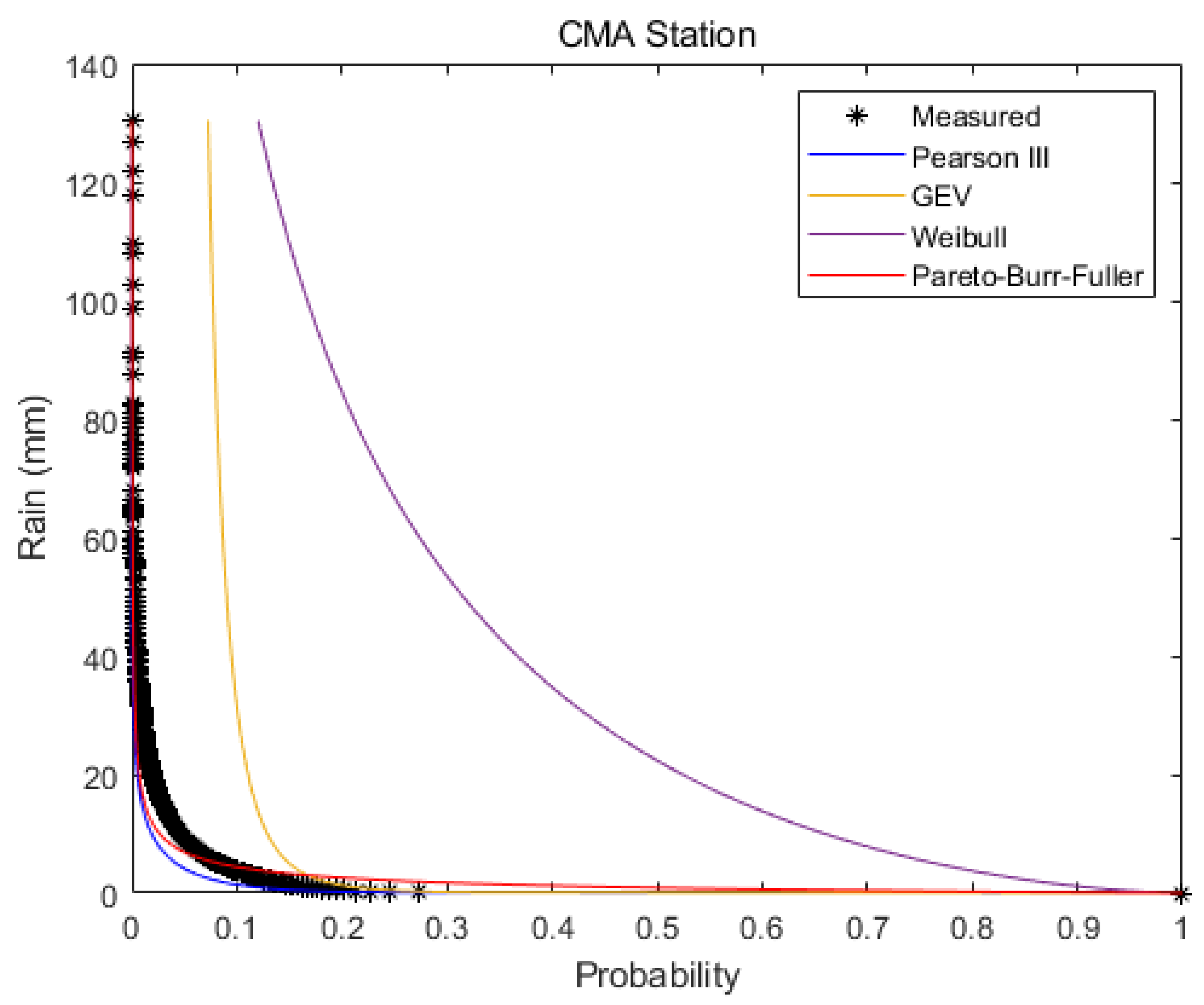
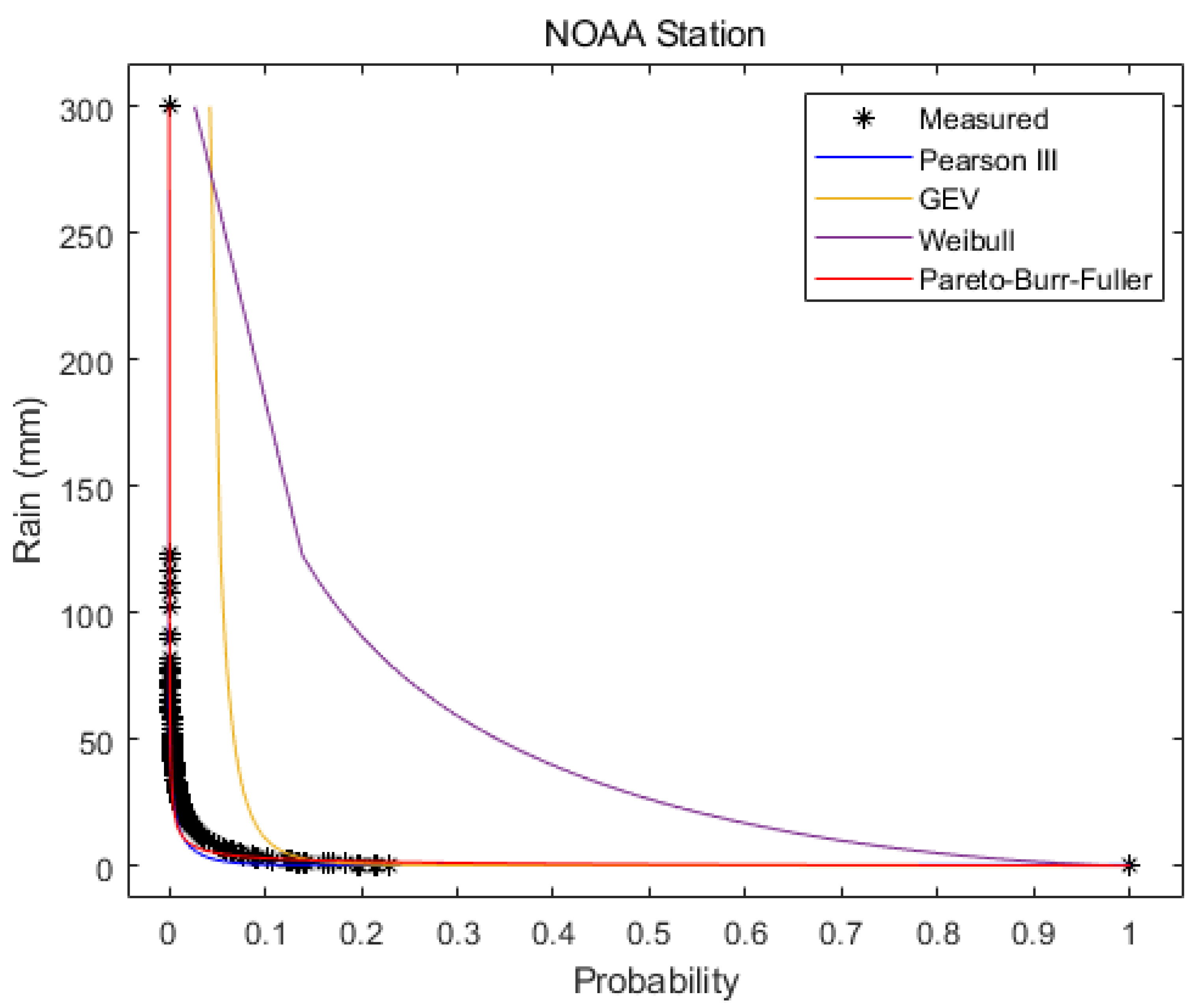
3.1. Frequency Distributions of the Daily Versus Wet-Day Series

For the complete daily time series of the CMA station, the Pearson type III model achieved the best accuracy with the corresponding NSE close to one, followed by the PBF model (Figure 2). With regards to the NOAA station, the accuracy of the Pearson III type model and PBF model were also better than GEV and Weibull distributions with the corresponding NSE value close to one (Figure 3). This was consistent with the findings from Ye [18]. Since the data with zero precipitation values should be removed for the Weibull distribution model [51], its curve was excluded. Though only used to handle the wet-day series, the Weibull distribution did not appear to fit with the local precipitation time series very well.

The analysis of the complete time series yielded superior results compared to the analysis conducted solely on the wet-day time series. The PDFs derived from the complete series exhibited significantly better fitting compared to the PDF derived from the wet-day series, using the observed complete series as the benchmark (

Table 1. The comparison of the NSE values of the four distributions based on the CMA data.

Distributions	NSE (Modeled Complete Series vs. Measured Complete Series)	NSE (Modeled Wet-Day Series vs. Measured Complete Series)	NSE (Modeled Wet-Day Series vs. Measured Wet-Day Series)
Pearson III	0.994	−0.2404	0.990
PBF	0.881	−0.5283	0.955
GEV	−3.85 × 104	−4.59 × 104	−7.06 × 105
Weibull	-	−207.5789	−71.68

and

Table 2. The comparison of the NSE values of the four distributions based on the NOAA data.

Distributions	NSE (Modeled Complete Series vs. Measured Complete Series)	NSE (Modeled Wet-Day Series vs. Measured Complete Series)	NSE (Modeled Wet-Day Series vs. Measured Wet-Day Series)
Pearson III	0.930	−0.2600	0.922
PBF	0.838	−0.6605	0.952
GEV	−2.03 × 1021	−2.47 × 1021	−2.34 × 103
Weibull	-	−246.7235	−62.20

). For the CMA station, when established from the complete series, the Pearson III, PBF, and GEV distributions achieved 514%, 260%, and 16% higher NSE values in fitting with the observed complete series, compared to those three distributions established from the wet series, respectively. For the NOAA station, the improvements of the Pearson III, PBF, and GEV distributions established from the complete daily series in fitting with the observed complete series were 458%, 227%, and 18%, respectively. This aligned with the previous study that the fitting could sometimes be enhanced without the need to separate dry and wet rainfall [24]. According to the analysis results, for daily rainfall, the Pearson type III distribution performed better than other distributions, while the PBF distribution also well generalized the complete daily series (Table 1 and Table 2). This is because the frequency analysis based on the complete daily time series considered dry spells between rain events and estimated the probability of rain on any given day. This comprehensive approach is more useful for practical applications such as runoff calculation and irrigation estimation than using only the wet-day series [52]. Interestingly, these findings align with the outcomes obtained from the analysis using the normal distribution [23].

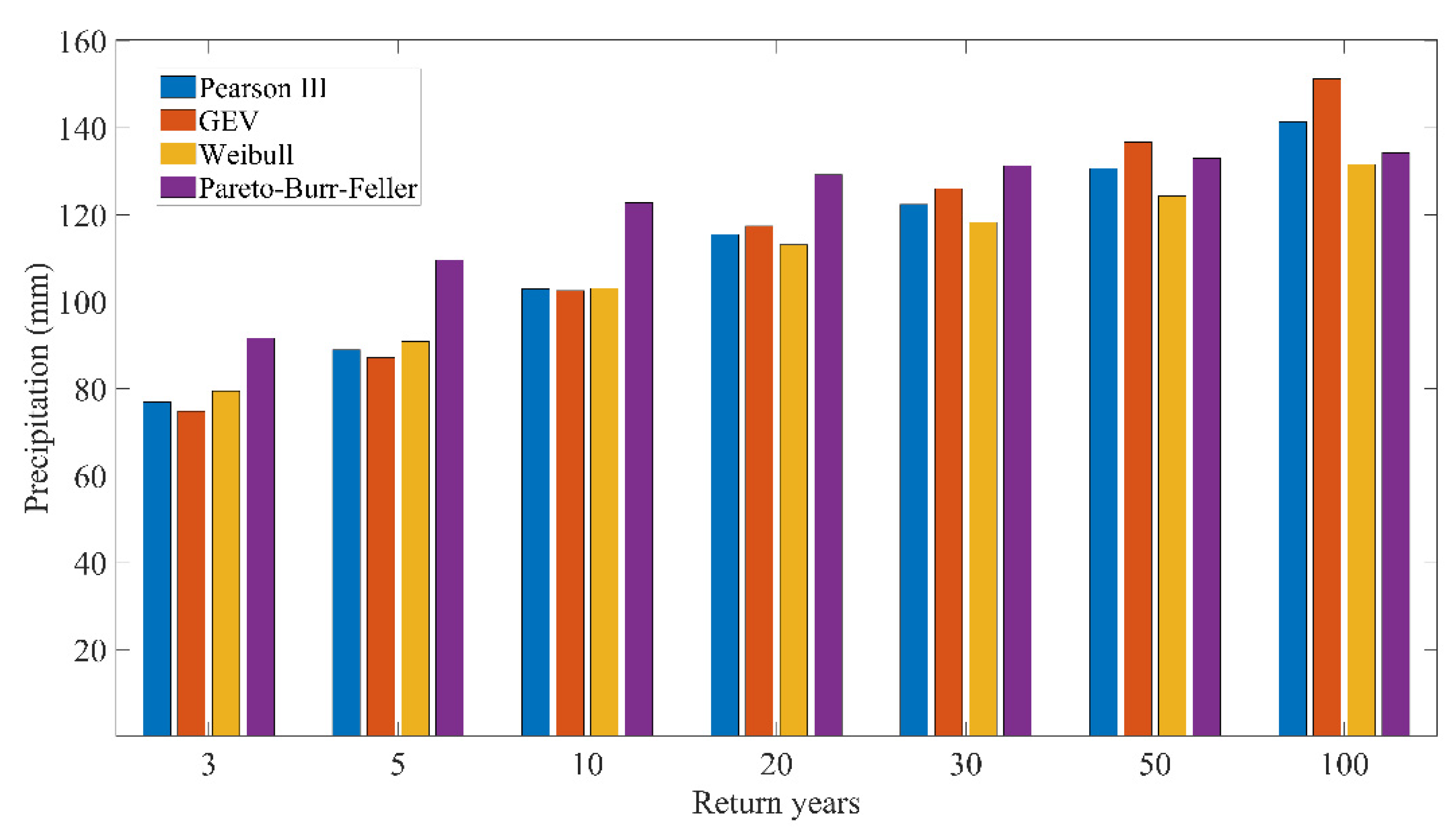
3.2. Return Periods Corresponding to the Daily Versus Wet-Day Series

The return periods of precipitation events affected the design of flood control and urban drainage systems. As mentioned above, Pearson type III distribution was more suitable for fitting the complete series of precipitation, so it was used to compute the return periods. Out of the 21,915 daily records of the CMA observation dataset, a total of 207 days had precipitation depths greater than 30.79 mm, which was approximately equal to 1% probability and then validated the aforementioned frequency analysis based on the Pearson type III distribution.

Again, compared with the return periods predicted based on the wet-day series, the prediction based on the complete time series of the CMA station took account of the factor of the dry spells between rain events, which could be practically significant for balancing the urban flooding risk management with the system efficiency and lifetime costs. If determined based on the wet series, the rain depth of the studied return periods was at least 75.67% higher than that determined from the complete daily series, indicating a significant overestimation of the real condition which includes both rainy and dry periods. Such overestimation became even larger as the recurrence decreased (

Table 3. The comparison of the rain depths of different recurrence intervals determined by the complete series and wet-day series based on Pearson III distribution for the CMA station.

Inputs	3Y	5Y	10Y	20Y	30Y	50Y	100Y
Complete Series	0.09	0.45	2.96	8.64	13.24	20.08	30.79
Wet-day Series	3.27	7.40	15.64	25.89	32.53	41.39	54.09

). It is, therefore, necessary to consider the chance of a rain occurrence before using the probability of a certain rain depth determined by the frequency analysis based on the wet days only. Ignoring the probability of whether raining or not would lead to significant over-prediction of surface runoff in the hydrologic calculations and over-investments in drainage designs that would be rarely operated at full capacity.

In this study, the earlier fits of the GEV distribution and Weibull distribution were found to be ineffective for daily series. In order to eliminate the possibility of any errors in the methods themselves, further investigations and analyses were conducted for annual maxima. The four probability models were adopted to estimate the return periods of the annual maximums (Figure 4). Since only the yearly maximum of every year was used, the issue of autocorrelation was mostly avoided, which made the estimated return periods and the corresponding rain depths comparable among the four models. So, the previous bad performance of the GEV and Weibull methods should be mainly caused by the mismatch between the models and the observations on a daily basis.

3.3. Threshold of Data Independence

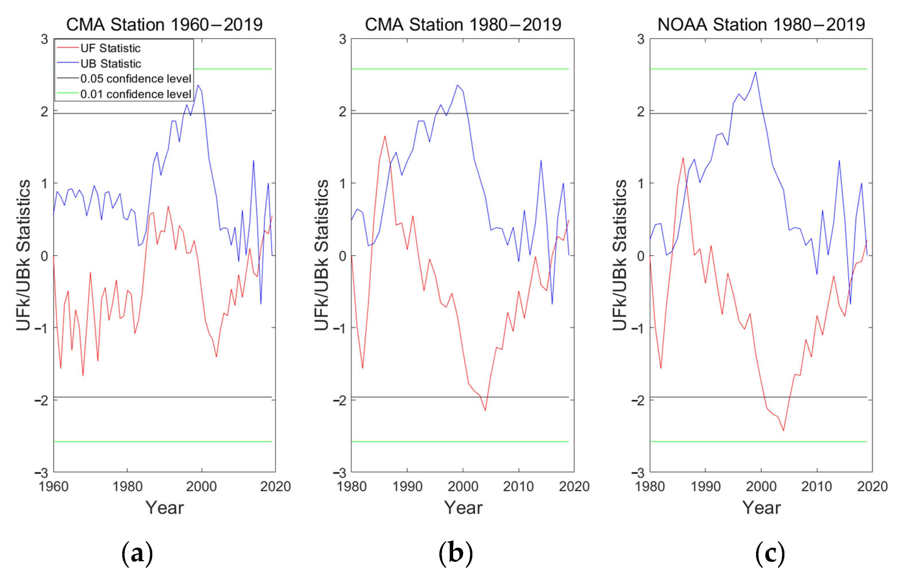
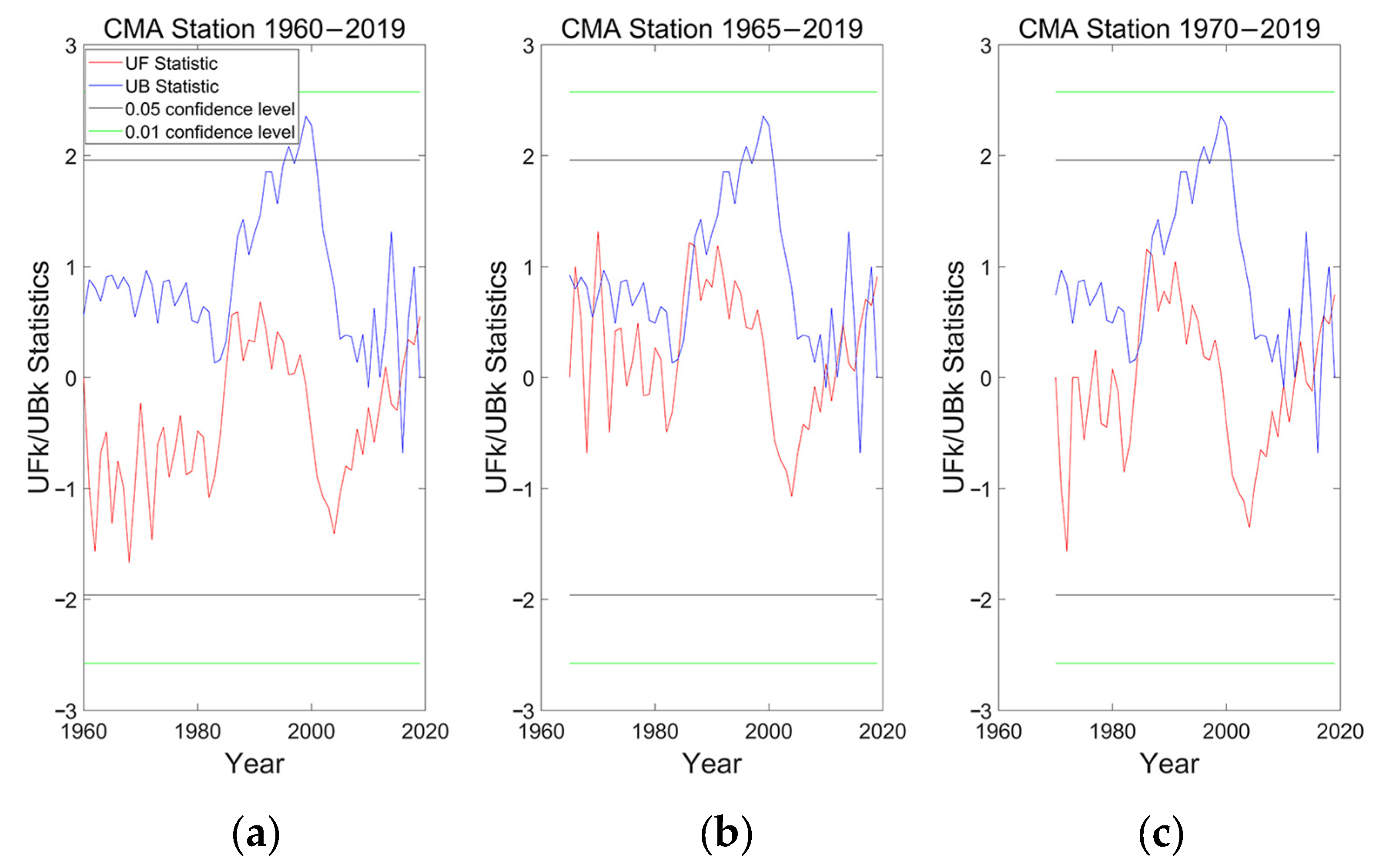
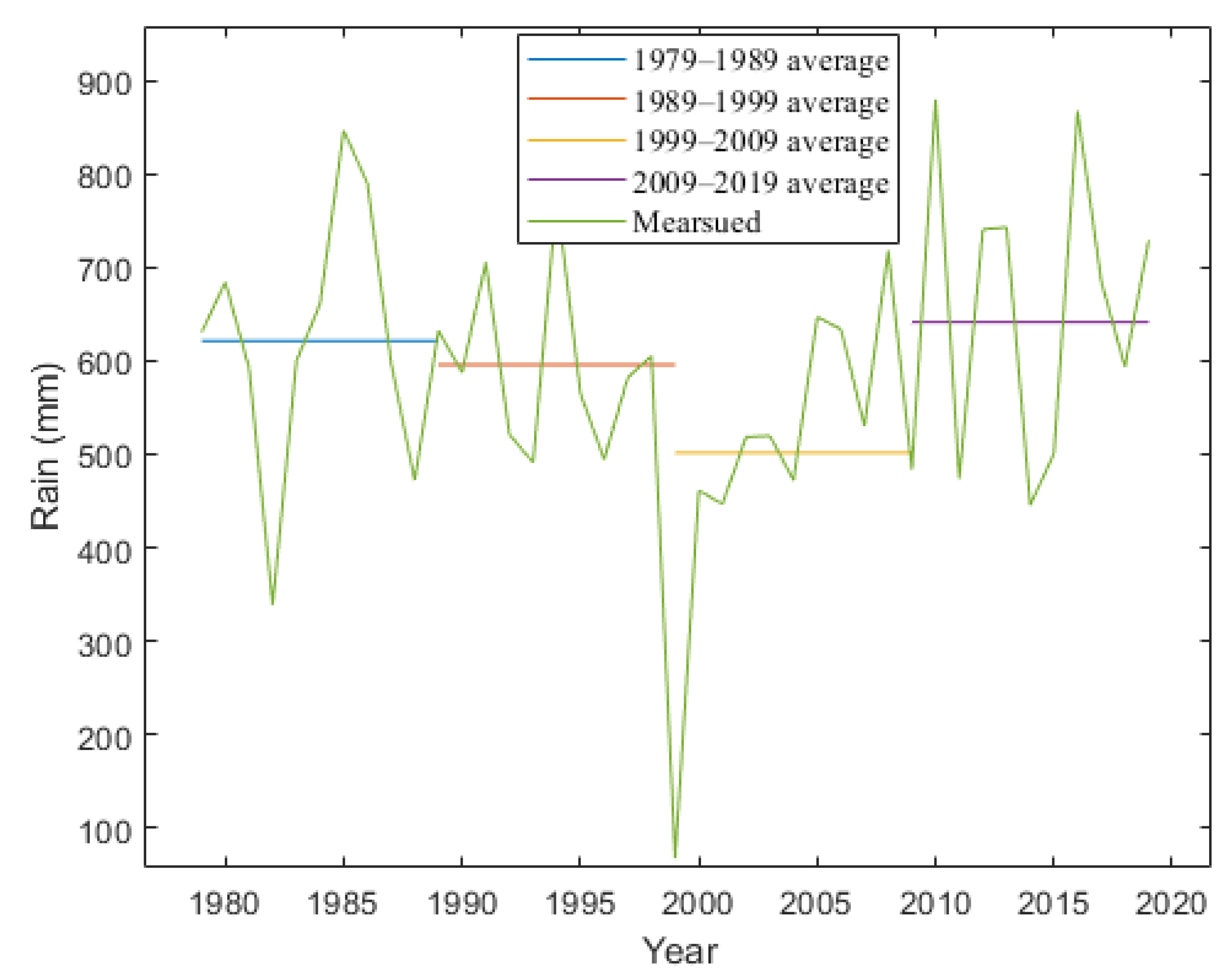
Based on this study, the daily time series were found to have a strong autocorrelation, but when the time series was expanded to an annual scale, the correlation tended to weaken, resulting in the independent time series (

Table 4. Test of serial correlation.

	$\frac{-1-1.645\sqrt{\mathit{n}-2}}{\mathit{n}-1}$	${\mathit{r}}_1$	$\frac{-1+1.645\sqrt{\mathit{n}-2}}{\mathit{n}-1}$
Wet daily series	−0.0112	0.1632	0.0111
Complete daily series	−0.0214	0.1307	0.0211
Annual extremes	−0.2293	−0.2037	0.1954

).

Conststently, the climacogram analysis not only supported this finding, but also showed a clear step threshold (k = 137) dividing the persistent time series from the antipersistent series. When the temporal scale k exceeded the threshold, the ending slope of the double logarithmic plot for the annual maxima was −0.62 (Figure 5), so the Hurst coefficient was 0.38 that fell into the range between 0 and 0.5, indicating that the time series became long-term antipersistent, or independent. Although a recent study indicated that the Hurst parameter, as a type of metric assessing the persistence, might lead to a false indication of data independence for the non-Gaussian time series [39], the annual maxima of this study followed a Gaussian distribution. On the other hand, when the temporal scale k was lower than the threshold, the data series became autocorrelated in terms of having a persistent structure. Such a threshold might be region dependent. This finding, therefore, proposed a practical means to validate the results of models such as the GEV that required data independence, and the threshold could be estimated to predetermine the lowest time step required for conducting the long-term trend tests.

As a longer time interval was considered, the serial independence of the time series gradually improved, and so did the NSE values of the GEV, as GEV required data independence [37]. The daily rainfall time series did not have a decent independence compared to the annual extremes (Table 4), which was the reason why the GEV models could not achieve a good fitting for the daily time series even if only the wet-day data were counted. Despite the prolonged time intervals between the observation points, the accuracy of the Pearson type III model was still quite stable and way better than the GEV models (Figure 6).

3.4. Trend Analysis

The MK tests were conducted for the CMA and NOAA stations, which indicate that intersection points between the UF and UB curves occurred in 1983, 1986, 2015, 2016, and 2018 at the NOAA station and in 2015, 2016, and 2018 at the CMA station (Figure 7). The common years were found as 2016 and 2018.

For the CMA station, the UF values in 2016 and 2018 were both greater than zero. An upward trend showed up right after the UF values exceeded zero in 2015, which was then considered the mutation year. The intersection points of the NOAA data were located in 1983, 1986, 2015, 2016, and 2018. Notably, the long-term negative UF values became positive in 2018, which was regarded as the mutation year.

The mutation years determined by the two stations appeared to be slightly different, which might be because the NOAA data had a shorter duration due to the ten-year data gap before 1980 (Figure 7). As the duration of the time series prolonged, the mutation points between the two stations became closer.

Through the analysis, it was found that the MK mutation test method was highly sensitive to the starting and end points of the time series to be analyzed. It is necessary to note that the UF had a positive sequence while the UB used the negative sequence of the rain series. So, if the starting point (or the endpoint) of the time series was picked differently, the UF and UB curves would shift in the reverse directions and intersect at new points. More importantly, the UF values of the same time range could also vary due to a different choice of the starting point, because the rise and fall of the UF curve mainly depends on the relation between S_k and E(S_k) in Equation (19). For instance, if the analysis started from 1960, the UF value around 1987 was slightly above 0.5 (Figure 7a), since the period 1960–1980 provided a decent magnitude of E(S_k) around 600 mm (Figure 8). But, if the starting point of the analysis window was picked at 1980, 20 years later than the previous window, the UF value around the same 1987 would jump to over 1.5 (Figure 7b), because of the lack of the period of 1960–1980 with the stable rainfall amounts led to a lower E(S_k) (Figure 8).

Similarly, if choosing 1960, 1965, and 1970 as the three starting points with the fixed endpoint, the MK tests led to significantly different mutation points (Figure 9), i.e., the total of the intersection points became 3, 13, and 7, respectively. When 2014, 2009, and 2004 were selected to be the 3 endpoints while the starting year was fixed at 1960, the total of the intersection points changed into 10, 15, and 9, respectively (Figure 10).

The ten-year averages of precipitation were calculated for the 40 years ranging from 1979 to 2019 (Figure 11 and Figure 12). It indicates that the 30-year period from 1979 to 2009 exhibited a descending trend, while the average precipitation of the decade from 2009 to 2019 significantly increased, which consolidates the previous finding concerning the mutation test. This could be further demonstrated by the 30-year comparison, in which the precipitation amount of any recurrence of the period of 1990–2019 was higher than that of 1960–1989 (Figure 13), indicating the increase in the magnitude of the local precipitation events. Correspondingly, the same level of precipitation could arrive in fewer return years in the recent 30 years (1990–2019) than the previous 30 years (1960–1989), indicating an acceleration of the frequency of the local precipitation events.

The increase in the average precipitation in the study area in Northeastern China might be related to the northward movement of the rain belt in China. Gao, et al. [53] through the study of 77 stations in 28° N–32° N found that China was considered to be in the range of the phenomenon of northward shift of the Meiyu rain belt. Liu, et al. [54] found that the rain belt moved northward and made rainfall increase in China north. Yun, Jianxin and Huatang [31] used 50-year rainfall data and proved that the rainfall in Northeastern China significantly increased after 2010, which was consistent with the previous finding in this study. It is then speculated that the reason why the increase in the northeast was related to the northward movement of the rain belt in northeast China.

A finding in this work was that the precipitation trend influenced the results of the rainfall frequency analysis. When the precipitation time series had an increasing trend, the NSE of the frequency analysis based on the Pearson III distribution was better than the time series having a descending trend from 1974 to 1982 (

Table 5. The NSE of different trends based on CMA station.

Time Series	Data Type	Trend	NSE	STD
1974–1982	Complete	Decreasing	0.9721	5.5297
1982–1990	Complete	Increasing	0.9946	6.1688
1974–1982	Wet day	Decreasing	0.9603	9.6523
1982–1990	Wet day	Increasing	0.9923	10.6826

Note: STD refers to standard deviation.

). The 20 years of time series (1970–1990) were extracted, during which the mutation point was 1982 (Figure 14). The 1982–1990 time series had an increasing trend while the 1974–1982 time series had a decreasing trend. At the same time, the NSE of the 1982–1990 time series was better than the 1974–1982 time series based on the complete rainfall time series.

3.5. Missing Gaps

Since a frequency analysis was often restrained by the missing data, this study also explored the relationship between data missing and the fitting effect by randomly inserting a spectrum of missing gaps into the CMA dataset on purpose. The sampling method of the K-permutations was adopted. Surprisingly, the results indicate that the accuracy of the curve fitting only started to significantly deteriorate only after the missing data took up 70%, which further indicates that the Pearson III distribution was quite robust in dealing with the precipitation time series for the study area. The data loss, therefore, should be controlled below 70% for a similar study.

The missing gaps between the wet-day time series were also tested based on the Pearson III distribution (

Table 6. Impact of missing data of complete daily series frequency analysis.

Loss Rate	NSE (Complete)	NSE (Wet Day)
10%	0.98	0.99
20%	0.97	0.99
30%	0.97	0.99
40%	0.97	0.99
50%	0.97	0.99
60%	0.97	0.99
70%	0.12	0.98
80%	0.31	0.99

). Different from the results of the complete time series, the wet-day series appeared not to be affected by the data missing. When the data missing rate achieved 80%, the NSE of the fitting result did not fall. The reason why the missing gaps affect the two datasets differently is due to the parameters of Pearson III distribution.

Within the rainfall dataset, the majority of the data were from dry days. During the verification process of missing data, a large portion of the non-rainy data was excluded, leading to variations in the standard deviation. In the case of the complete time series, with the increase in the number of missing data, the standard deviation gradually exhibited fluctuations to various degrees, which then passed to the C_s and C_v. In the unbiased estimate formula (Equation (3)), as the standard deviation with a cubic exponent decreased, the influence of the perturbation in the time series on the C_s value would be amplified (Equation (3)) causing a highly variable C_s curve (Figure 15). The fluctuations of those parameters eventually influenced the results of the frequency analysis based on the complete series. Therefore, when analyzing the probability of rainfall based on the complete time series, special attention should be paid to the amount of missing data because the calculated parameters based on the complete time series tend to have greater fluctuation on the derived PDFs.

The threshold of the 70% loss rate was expected to be influenced by the fraction of the dry days within the dataset. This finding may hold true for continental climates and dry regions where the dry days took up the majority of the time series dataset (72.6% in this study). As the time series included more dry days, such as dry Northeastern China, the threshold of loss rate would gradually decrease; while in wet climates where the dry days were much fewer, the threshold of loss rate would gradually increase, i.e., the frequency analysis was less affected by the data missing.

4. Conclusions

This work aimed to develop the precipitation probability distribution fitting with complete daily series, which could provide the actual probability of rainfall on any given day regardless of knowing in advance if it is a rainy/wet day or if it belongs to a wet season. Changchun, Jilin Province, China was picked as a case study to conduct the frequency analysis and trend analysis of the recent precipitation events in Northeastern China. An approximate 60 years of precipitation time series were collected from the CMA and NOAA stations. Four types of probability distributions were tested and compared, which included Pearson type III, GEV, Weibull, and PBF distributions. The M-K tests were further adopted to analyze the historic trend. The major findings were listed as follows.

(1)

The use of complete time series in precipitation frequency analysis gave more realistic estimates of probabilities than the traditional methods relying on rainy days only. Based on the two separate weather stations, the Pearson III and PBF distributions established from the complete daily series were at least 458% and 227% more accurate in fitting with the observed complete daily series than the distributions established from the wet-day-only series. The return periods of historic rainfall should also be determined from the complete daily series rather than the wet-day-only series, since the latter might overestimate the rain depths of the studied return periods by at least 76% if the depths of the corresponding return periods are more closely represented by the real condition.

(2)

A clear threshold of 137 days was found in this study to separate the persistent or autocorrelated time series from the antipersistent or independent time series based on the climacogram analysis. This threshold, possibly varied case by case, was proposed as a practical way to validate the GEV model or as such required data independence and predetermine the lowest time step for the long-term trend tests.

(3)

The choice of the starting and ending points had a significant influence on the M-K test and easily led to different mutation points for trend analysis.

(4)

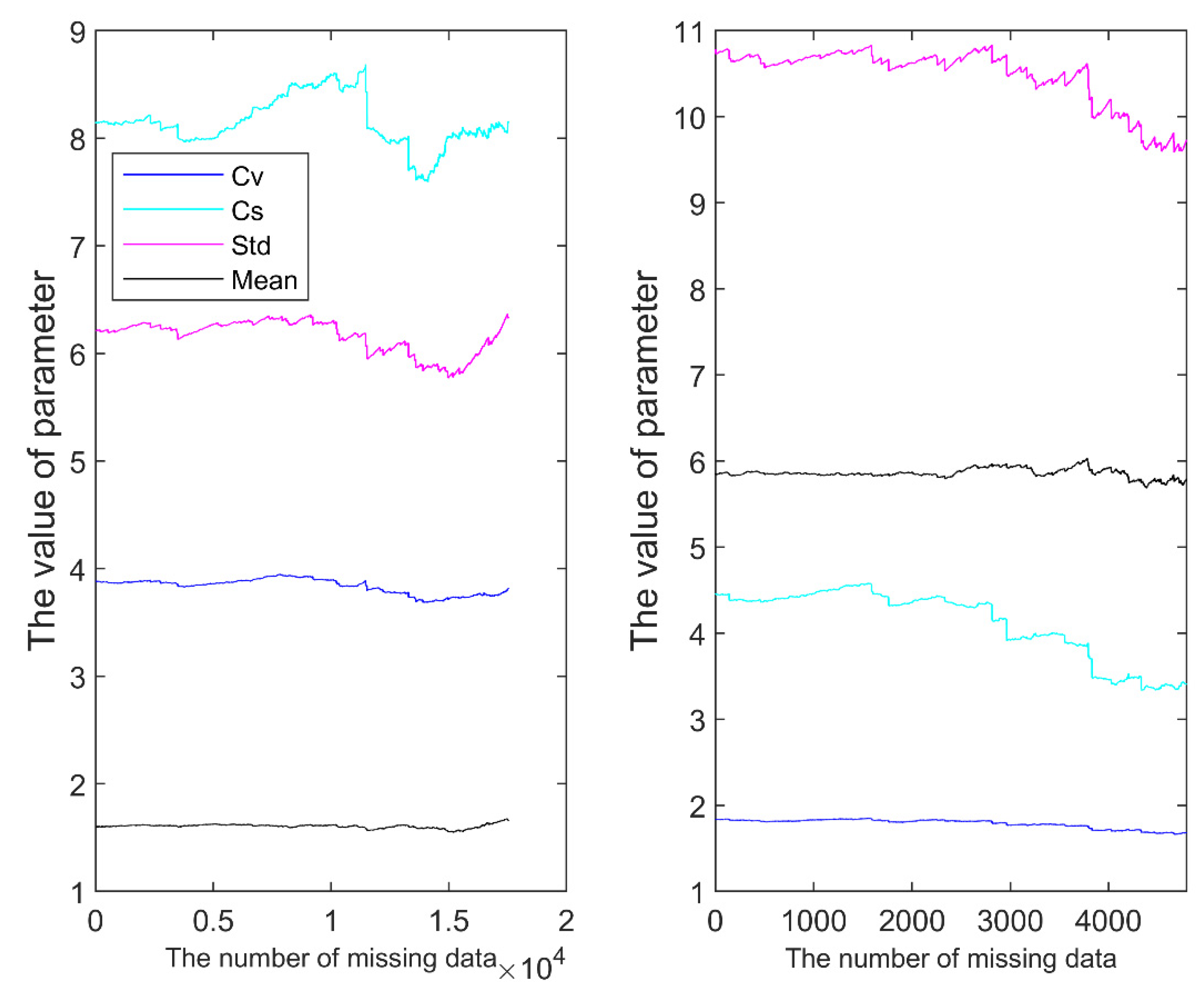
The test of K-permutation sampling revealed that the lack of data would affect the accuracy of the frequency analysis only after the missing data reached 70% of the whole dataset. The wet-day series were less affected by the data gaps than the complete time series.

Based on the significant difference between the precipitation frequency analyses conducted by the complete daily series and the wet-day-only series, this work strongly argued that the complete daily series better represented the real condition and, therefore, should be used for the frequency analysis by the designs and constructions of the flood control and drainage systems.

References

1. Zhong, S.; Zhuang, Y.; Hu, S.; Chen, Z.; Ding, W.; Feng, Y.; Deng, T.; Liu, X.; Zhang, Y.; Xu, D.; et al. Verification and Assessment of Real-time Forecasts of Two Extreme Heavy Rain Events in Zhengzhou by Operational NWP Models. J. Trop. Meteorol. 2021, 27, 406–417. [Google Scholar]
2. Benson, M.A. Uniform Flood-Frequency Estimating Methods for Federal Agencies. Water Resour. Res. 1968, 4, 891–908. [Google Scholar] [CrossRef]
3. Fréchet, M. Sur la loi de probabilité de l’écart maximum. Ann. Soc. Math. Pol. 1927, 6, 93–116. [Google Scholar]
4. Weibull, W. A statistical distribution function of wide applicability. J. Appl. Mech. 1951, 18, 293–297. [Google Scholar] [CrossRef]
5. Gumbel, E.J. Statistics of Extremes; Courier Corporation: North Chelmsford, MA, USA, 1958. [Google Scholar]
6. Burr, I.W. Cumulative frequency functions. Ann. Math. Stat. 1942, 13, 215–232. [Google Scholar] [CrossRef]
7. Jenkinson, A.F. The frequency distribution of the annual maximum (or minimum) values of meteorological elements. Q. J. R. Meteorol. Soc. 1955, 81, 158–171. [Google Scholar] [CrossRef]
8. Serinaldi, F.; Petroselli, A.; Grimaldi, S. A continuous simulation model for design-hydrograph estimation in small and ungauged watersheds. Hydrol. Sci. J. 2012, 57, 1035–1051. [Google Scholar]
9. Grimaldi, S.; Volpi, E.; Langousis, A.; Papalexiou, S.M.; De Luca, D.L.; Piscopia, R.; Nerantzaki, S.D.; Papacharalampous, G.; Petroselli, A. Continuous hydrologic modelling for small and ungauged basins: A comparison of eight rainfall models for sub-daily runoff simulations. J. Hydrol. 2022, 610, 127866. [Google Scholar] [CrossRef]
10. Hosking, J.R.M.; Wallis, J.R. Regional Frequency Analysis; Cambridge University Press: Cambridge, UK, 1997. [Google Scholar]
11. Lin, B.; Bonnin, G.M.; Martin, D.L.; Parzybok, T.; Yekta, M.; Riley, D. Regional Frequency Studies of Annual Extreme Precipitation in the United States Based on Regional L-Moments Analysis. In Proceedings of the World Environmental and Water Resource Congress 2006: Examining the Confluence of Environmental and Water Concerns, Omaha, NB, USA, 21–25 May 2006. [Google Scholar]
12. Hosking, J.R. L-moments: Analysis and estimation of distributions using linear combinations of order statistics. J. R. Stat. Soc. Ser. B Methodol. 1990, 52, 105–124. [Google Scholar] [CrossRef]
13. Wilks, D. Multisite generalization of a daily stochastic precipitation generation model. J. Hydrol. 1998, 210, 178–191. [Google Scholar] [CrossRef]
14. Naghavi, B.; Yu, F.X. Regional frequency analysis of extreme precipitation in Louisiana. J. Hydraul. Eng. 1995, 121, 819–827. [Google Scholar] [CrossRef]
15. Xie, Y. Urban drainage and waterlogging disaster prevention planning. China Water Wastewater 2013, 29, 105–108. [Google Scholar]
16. Shao, Y.-m.; Shao, D.-n.; Ma, J.-s. Practice and Suggestion on New Generation of Formula of Urban Rainstorm Intensity. China Water Wastewater 2012, 28, 19–22. [Google Scholar]
17. Yifan, J.; Songbai, S. Optimization of flood frequency distribution parameter estimation method based on TL-moments. Water Resour. Prot. 2021, 37, 34–39. [Google Scholar]
18. Ye, L.; Hanson, L.S.; Ding, P.; Wang, D.; Vogel, R.M. The probability distribution of daily precipitation at the point and catchment scales in the United States. Hydrol. Earth Syst. Sci. 2018, 22, 6519–6531. [Google Scholar] [CrossRef]
19. Yevjevich, V. Probability and Statistics in Hydrology; Water Resources Publications: Highlands Ranch, CO, USA, 1972. [Google Scholar]
20. El Adlouni, S.; Bobée, B.; Ouarda, T.B.M.J. On the tails of extreme event distributions in hydrology. J. Hydrol. 2008, 355, 16–33. [Google Scholar] [CrossRef]
21. Koutsoyiannis, D. Uncertainty, entropy, scaling and hydrological stochastics. 1. Marginal distributional properties of hydrological processes and state scaling/Incertitude, entropie, effet d’échelle et propriétés stochastiques hydrologiques. 1. Propriétés distributionnel. Hydrol. Sci. J. 2005, 50, 381–404. [Google Scholar]
22. Koutsoyiannis, D. Uncertainty, entropy, scaling and hydrological stochastics. 2. Time dependence of hydrological processes and time scaling/Incertitude, entropie, effet d’échelle et propriétés stochastiques hydrologiques. 2. Dépendance temporelle des processus hydrologiques et échelle temporelle. Hydrol. Sci. J. 2005, 50, 405–426. [Google Scholar]
23. Shoji, T.; Kitaura, H. Statistical and geostatistical analysis of rainfall in central Japan. Comput. Geosci. 2006, 32, 1007–1024. [Google Scholar] [CrossRef]
24. Dimitriadis, P.; Koutsoyiannis, D. Stochastic synthesis approximating any process dependence and distribution. Stoch. Environ. Res. Risk Assess. 2018, 32, 1493–1515. [Google Scholar] [CrossRef]
25. Iliopoulou, T.; Koutsoyiannis, D. Projecting the future of rainfall extremes: Better classic than trendy. J. Hydrol. 2020, 588, 125005. [Google Scholar] [CrossRef]
26. Koutsoyiannis, D.; Montanari, A. Negligent killing of scientific concepts: The stationarity case. Hydrol. Sci. J. 2015, 60, 1174–1183. [Google Scholar] [CrossRef]
27. Borah, P.; Hazarika, S.; Prakash, A. Assessing the state of homogeneity, variability and trends in the rainfall time series from 1969 to 2017 and its significance for groundwater in north-east India. Nat. Hazards 2022, 111, 585–617. [Google Scholar] [CrossRef]
28. Said, M.; Komakech, H.C.; Munishi, L.K.; Muzuka, A.N.N. Evidence of climate change impacts on water, food and energy resources around Kilimanjaro, Tanzania. Reg. Environ. Chang. 2019, 19, 2521–2534. [Google Scholar] [CrossRef]
29. Suescún, D.; Villegas, J.C.; León, J.D.; Flórez, C.P.; García-Leoz, V. Vegetation cover and rainfall seasonality impact nutrient loss via runoff and erosion in the Colombian Andes. Reg. Environ. Chang. 2017, 17, 827–839. [Google Scholar] [CrossRef]
30. Lal, M. Implications of climate change in sustained agricultural productivity in South Asia. Reg. Environ. Chang. 2011, 11, 79–94. [Google Scholar] [CrossRef]
31. Yun, P.; Jianxin, X.; Huatang, R. The Variations of Rainfall Belt and Its Impact in China. China Rural Water Hydropower 2015, 5, 45–48. [Google Scholar]
32. Li, W.; Zhao, S.; Chen, Y.; Wang, Q.; Ai, W. State of China’s Climate in 2020. Atmos. Ocean. Sci. Lett. 2021, 14, 9–14. [Google Scholar] [CrossRef]
33. Li, Q. Comparative study of parameter estimation methods for Pearson type III curves based on numerical integration. Water Resour. Plan. Des. 2018, 12, 54–59. [Google Scholar]
34. He, S.; Li, Z.; Liu, X. An improved GEV boosting method for imbalanced data classification with application to short-term rainfall prediction. J. Hydrol. 2023, 617, 128882. [Google Scholar] [CrossRef]
35. Koutsoyiannis, D. Statistics of extremes and estimation of extreme rainfall: I. Theoretical investigation. Hydrol. Sci. J. 2004, 49, 575–590. [Google Scholar] [CrossRef]
36. Montoya, J.; Díaz-Francés, E.; Figueroa, G. Estimation of the reliability parameter for three-parameter Weibull models. Appl. Math. Model. 2019, 67, 621–633. [Google Scholar] [CrossRef]
37. Reza Najafi, M.; Moradkhani, H. Analysis of runoff extremes using spatial hierarchical Bayesian modeling. Water Resour. Res. 2013, 49, 6656–6670. [Google Scholar] [CrossRef]
38. Dimitriadis, P.; Koutsoyiannis, D. Climacogram versus autocovariance and power spectrum in stochastic modelling for Markovian and Hurst–Kolmogorov processes. Stoch. Environ. Res. Risk Assess. 2015, 29, 1649–1669. [Google Scholar] [CrossRef]
39. Iliopoulou, T.; Koutsoyiannis, D. Revealing hidden persistence in maximum rainfall records. Hydrol. Sci. J. 2019, 64, 1673–1689. [Google Scholar] [CrossRef]
40. Koutsoyiannis, D. HESS Opinions “A random walk on water”. Hydrol. Earth Syst. Sci. 2010, 14, 585–601. [Google Scholar] [CrossRef]
41. Hurst, H.E. Long-term storage capacity of reservoirs. Trans. Am. Soc. Civ. Eng. 1951, 116, 770–799. [Google Scholar] [CrossRef]
42. Kendall, M.G. Rank Correlation Methods; J.F. Griffin Publishing: Williamstown, MA, USA, 1948. [Google Scholar]
43. Mann, H.B. Nonparametric tests against trend. Econom. J. Econom. Soc. 1945, 13, 245–259. [Google Scholar] [CrossRef]
44. Hamed, K.H.; Rao, A.R. A modified Mann-Kendall trend test for autocorrelated data. J. Hydrol. 1998, 204, 182–196. [Google Scholar] [CrossRef]
45. Sen, P.K. Estimates of the regression coefficient based on Kendall’s tau. J. Am. Stat. Assoc. 1968, 63, 1379–1389. [Google Scholar] [CrossRef]
46. Yue, S.; Wang, C. The Mann-Kendall test modified by effective sample size to detect trend in serially correlated hydrological series. Water Resour. Manag. 2004, 18, 201–218. [Google Scholar] [CrossRef]
47. Yildirim, G.; Rahman, A. Homogeneity and trend analysis of rainfall and droughts over Southeast Australia. Nat. Hazards 2022, 112, 1657–1683. [Google Scholar] [CrossRef]
48. Yuan, J.; Xu, Y.; Wu, L.; Wang, J.; Wang, Y.; Xu, Y.; Dai, X. Variability of precipitation extremes over the Yangtze River Delta, Eastern China, during 1960–2016. Theor. Appl. Climatol. 2019, 138, 305–319. [Google Scholar] [CrossRef]
49. Yilmaz, B. Analysis of hydrological drought trends in the GAP region (southeastern Turkey) by Mann-Kendall test and innovative sen method. Appl. Ecol. Environ. Res. 2019, 17, 3325–3342. [Google Scholar] [CrossRef]
50. Wang, J. Determining the most accurate program for the Mann-Kendall method in detecting climate mutation. Theor. Appl. Climatol. 2020, 142, 847–854. [Google Scholar] [CrossRef]
51. Wang, C.; Lin, K. Fitting method of Weibull equation: Application of optimum seeking method to the fitting of the progressive curve of plant disease. J. South China Agric. Univ. 1986, 1, 17–20. [Google Scholar]
52. Wei, X.G.Z. The analysis for the drought law in Changchun region. Jilin Water Resour. 2008, 6, 19–22. [Google Scholar]
53. Gao, Q.; Sun, Y.; You, Q. The northward shift of Meiyu rain belt and its possible association with rainfall intensity changes and the Pacific-Japan pattern. Dyn. Atmos. Ocean. 2016, 76, 52–62. [Google Scholar] [CrossRef]
54. Liu, J.; Shen, Z.; Chen, W.; Chen, J.; Zhang, X.; Chen, J.; Chen, F. Dipolar mode of precipitation changes between North China and the Yangtze River valley existed over the entire Holocene: Evidence from the sediment record of Nanyi Lake. Int. J. Climatol. 2021, 41, 1667–1681. [Google Scholar] [CrossRef]
Figure 1. Location of the CMA station and NOAA station.
Sustainability 15 13136 g001
Figure 2. The fitting of the CMA data with the Pearson type III, GEV, Weibull, and PBF probability distribution curves.
Sustainability 15 13136 g002
Figure 3. The fitting of the NOAA data with the Pearson type III, GEV, Weibull, and PBF probability distribution curves.
Sustainability 15 13136 g003
Figure 4. Prediction of the return periods of the annual maximums based on the CMA station.
Sustainability 15 13136 g004
Figure 5. Climacogram of the standard deviation of the averaged process vs. the averaging timescale.
Sustainability 15 13136 g005
Figure 6. Relationship between the selected time intervals of the wet-day observations and the NSE. Note: the order of magnitude of Y-axis is 105. The minimum NSE of Pearson III was 0.94 and the maximum of Pearson III was 0.99.
Sustainability 15 13136 g006
Figure 7. The MK test results of the CMA station and NOAA station. Note: UF and UB are standard normal distribution statistics. (Note: (a) CMA rain data of 1960 to 2019, (b) CMA rain data of 1980 to 2019, (c) NOAA rain data of 1980 to 2019.
Sustainability 15 13136 g007
Figure 8. The total annual rainfall of the CMA station.
Sustainability 15 13136 g008
Figure 9. The MK test result of different lengths of time series (starting point varied). Note: UF and UB are standard normal distribution statistics.(Note: (ac) have different starting points, so there are different intersection points).
Sustainability 15 13136 g009
Figure 10. The MK test result of different lengths of time series (starting point varied). Note: UF and UB are standard normal distribution statistics. (Note: (ac) have different ending points, so there are different intersection points).
Sustainability 15 13136 g010
Figure 11. Ten-year averages of the rainfall data at the CMA station.
Sustainability 15 13136 g011
Figure 12. Ten-year averages of the rainfall data at the NOAA station.
Sustainability 15 13136 g012
Figure 13. Pearson III prediction of the return periods of the annual maximum for the periods of 1960–1989 and 1990–2019 at the CMA station.
Sustainability 15 13136 g013
Figure 14. The MK test result of 1970–1990 based on CMA station.
Sustainability 15 13136 g014
Figure 15. The impact of missing data on two data parameters (left: complete time series; right: wet-day time series).
Sustainability 15 13136 g015