Optimization of Urban Road Green Belts under the Background of Carbon Peak Policy

Abstract

To explore the reasonable width of urban road green belts under the background of carbon peak policy and provide quantitative design guidance for urban green-belt planning, a closed-loop design that integrates urban traffic, carbon emissions, urban greening, and carbon absorption was established at the road network level. First, the factors affecting urban transport carbon emissions were analyzed from the aspects of environment, economy, population, and technology. A carbon emission prediction model was constructed based on the STIRPAT (stochastic impacts by regression on population, affluence, and technology) model. The path of the carbon peak in the transportation sector was simulated. A scenario under the carbon peak target was designed to determine the development trend of each factor. The layout forms and design requirements of urban road greening were then summarized. The annual carbon sequestration amounts of different plant types were calculated. An objective optimization model was constructed with the lowest cost of greening as the objective function. The constraint conditions specify that the carbon absorption be greater than the carbon emissions, in addition to specifying the basic greening design requirements. Finally, an empirical study was conducted on a road network area in Xi’an. According to the results, the traffic carbon emissions of Xi’an City will be 2.71 Mt in 2025, with road traffic accounting for 1.94 Mt. Without considering the road-measurement green-width constraint, the proportions of the road green belt for six road classes and the red-line width under the carbon peak target are 0.31, 0.33, 0.40, 0.22, 0.21, and 0.23. These research results provide a quantitative and reliable basis for designing the width of an urban green belt under the background of carbon peak policy. Under proportion restrictions, road greening yields better performance by considering both aesthetics and road characteristics.

1. Introduction

Private cars are widely favored by travelers because they are fast, comfortable, private, and capable of door-to-door travel. The number of private cars owned in China and their travel distance is rapidly increasing, with national motor vehicle ownership reaching 372 million vehicles in 2020, similar to that in the United States, with both tied for first place in the world. Urban transportation is under tremendous pressure, and urban environmental problems cannot be overlooked. Carbon emissions from transportation account for 15% of the country’s final carbon emissions, of which road traffic accounts for 72%, ranking second only to electricity [1]. Thus, the problem of carbon emissions urgently needs to be solved [2]. Countries worldwide are actively exploring the use of transportation demand management (TDM) strategies, including public transport priority and driving restriction policies, to relieve urban traffic pressure and reduce environmental pollution, thereby promoting the sustainable development of cities and achieving the goal of “double carbon” [3,4]. China’s 14th Five-Year Plan has for the first time specified the timeline and roadmap for China to achieve peak carbon and carbon neutrality and proposes to “implement the 2030 national autonomous contribution target for addressing climate change, formulate an action plan to achieve peak carbon emissions by the year 2030, and strive to achieve carbon neutrality by the year 2060”. Carbon peak is a prerequisite and foundation for carbon neutrality. Therefore, the research on urban traffic management and emission-reduction strategy based on the carbon peak target has become focal in the transportation and environment fields. Specifically, analyzing the carbon emissions associated with transportation and carbon sequestration under the dual carbon targets is crucial. A net-zero carbon system, in which the carbon emission is equal to carbon sequestration, means carbon neutrality has been achieved [5]. A carbon peak is achieved when the difference between carbon emission and carbon absorption reaches its peak. Therefore, the realization of dual carbon targets is closely related to carbon emission and carbon sequestration, which should be simultaneously studied within a given system.

Researchers have analyzed and tested the carbon emission peak in the traffic [6,7], energy and power [8,9], and landscaping fields [10]. Many previous methods such as structural decomposition analysis (SDA), the logarithmic mean Divisia index (LMDI), and the stochastic impact by regression on population, affluence, and technology (STIRPAT) model have been employed to examine the social and economic driving forces of anthropogenic environmental degradation [11,12,13,14,15]. Among these, the LMDI and STIRPAT are the two most widely used techniques for examining such drivers. The STIRPAT model, which is derived from the IPAT model, has been widely employed to analyze the driving force of energy consumption, CO₂ emission, and ecological footprints [16,17]. Compared with the LMDI model, the STIRPAT model can examine more factors and provide more detailed and reliable information for shaping environment friendly strategies [18,19]. The STIRPAT model allows for the expansion of the model to improve its analysis and interpretation ability by adding, subtracting, and decomposing factors, and can also eliminate the effects of proportional changes [20]. The STIRPAT model or improved STIRPAT model, which can consider many influence factors, is used to test the carbon emission peak and carbon neutrality [21,22,23,24,25,26]. Population, energy intensity, industrial structure, urbanization level, investment in fixed assets, urbanization, vehicle ownership, and gross domestic product (GDP) per capita, among other influencing factors, are often utilized in the STIRPAT model to predict carbon emissions [27,28]. Machine-learning methods have also been used to predict carbon emission, but they require large amounts of data, and because they are black boxes, continuously determining the nonlinear changing trend of the influence of independent variables on dependent variables is difficult [29]. Notwithstanding, exploring the carbon peak scenario is the key to elucidating the development trend of each influencing factor and determining the year of carbon peak as well as the control amount [26].

Planting trees can offset the carbon dioxide produced by human activities. Trees are also essential for ecological management, particularly in urban and periurban forests, and their potential to consistently absorb excessive anthropogenic NOx, which is considered the main air pollutant in China [30], has attracted the attention of governments and scientists [31]. According to a study by the State Forestry Administration, a single tree can absorb and store 4–18 kg of CO₂ per year. The latest research results published in Nature [32] by scientists from multiple countries reveal that China’s terrestrial ecosystems absorbed an average of about 1.11 billion tons of carbon (carbon sink) from 2010 to 2016, absorbing 45% of anthropogenic carbon emissions during the same period. The urban green space system is a natural carbon sink and is ecologically critical in the urban ecosystem [33,34]. Yushardi [35] revealed that the amount of carbon emissions in an area depends on the number of vehicles operating on main roads, residential roads, and terminals, among others. Greening can absorb large quantities of carbon emissions and reduce carbon dioxide gas in the urban road network. However, direct carbon sequestration by urban green space has a limited effect on reducing overall urban CO₂ emissions. Therefore, the carbon sequestration effect of green patches can still be improved through reasonable tree planting [36]. Tae-Yeol [37] found that a median strip width of 3.0 m was the most preferred for low-carbon green network roads, whereas shrubs, followed by small shrubs and trees, were the most preferred for greening. However, these studies were based on road sections and included little consideration of the carbon emission targets of the nation. Therefore, based on the principle of the joint management of carbon emissions and carbon sequestration, quantification analysis for the reasonable planting of urban road green belts based on traffic carbon emissions and dual carbon targets needs to be extended. Moreover, extending the research area from road sections to road networks in the future is of interest. These research results can be useful for greening planning not only for the field of landscaping but also for that of traffic.

Considering the rapid development of urban transportation and dual carbon target policy, balancing urban transportation development and ecological environmental protection, reducing the negative effects of traffic pollution on residents’ health and the urban environment, and adapting to urban development needs necessitate establishing an optimal relationship among urban transportation, carbon emissions, and road greening demand. This optimal relationship and the corresponding suggestions for optimal road greening design should be considered by both traffic planners and urban environmental designers. The optimal width, total percentage, and minimum cost of green belts can be quantitatively determined for different road classes, road red lines, and green belt types. Finally, a case study is conducted in a road network area of Xi’an to verify the feasibility and validity of the model.

The remainder of this paper is organized as follows. Section 2 describes the use of the STIRPAT model to obtain the carbon peak scenario. Section 3 describes the optimization of urban road green belts while considering the carbon peak. A case study is described in detail in Section 4. The final section summarizes the main findings and proposes future research directions.

2. Carbon Emission Prediction Based on the STIRPAT Model under the Background of Carbon Peak

2.1. STIRPAT Model

STIRPAT (stochastic impacts by regression on population, affluence, and technology) is an expandable stochastic environment influence assessment model [21,22,23,24,25] that examines the intrinsic relationship between population, affluence, and technology. Lin [38] mentioned that the main driving factors of environmental impact are population, affluence, and energy intensity, as shown in the following equation.

$$I=\alpha P^{{\beta }_1}{A}^{{\beta }_2}{T}^{{\beta }_3}ϵ$$

(1)

where I represents environmental pressure, expressed as carbon emissions; P represents population size; A represents affluence, expressed as GDP per capita; T represents technology, using the energy consumption intensity calculated from the energy consumption divided by the GDP [39]; $\alpha$ is a constant; β is the estimated coefficient of the variable parameter, which represents the elasticity of P, A, and T; and $ϵ$ is the error term.

To maintain data stationarity, facilitate calculation, eliminate the problem of magnitude, and reduce covariance and heteroskedasticity [40], the model can be transformed into the following linear logarithmic arithmetic form by taking the natural logarithm on both sides of the variables, which is shown in Equation (2).

$$lnI=ln\alpha +{\beta }_{1}lnP+{\beta }_{2}lnA+{\beta }_{3}lnT+lnϵ$$

(2)

where I, P, A, T, $\alpha$, β₁, β₂, β₃, and $ϵ$ are same as those in Equation (1). In logarithmic form, the coefficients represent the ${\beta }_1$% change in the driving environmental factor I for every 1% change in the variable, etc.

2.2. Factors Influencing Carbon Emissions of Urban Transportation

This paper divides the variables into four elemental categories, namely environmental, economic, demographic, and technological, and considers urban as well as road characteristic indicators [27,41], as detailed in

Table 1. Influencing Factors of Urban Traffic Carbon Emission.

Variable	Definition
Sidewalk density	Sidewalk area/Urban area
Land mix	Degree of land-type mixing (The Shannon diversity index was used as a measure of urban land use, with the formula C = ∑(Ui·ln(Ui)); where Ui is the proportion of the ith land type, and the larger the value of H, the higher the degree of land-type mixing.)
Compactness	Using land-use compactness, economic compactness, population compactness, and transportation compactness to reflect (Refer to [42])
Employment-to-occupancy ratio	The ratio of the number of jobs to the number of people living within a certain area
Number of private vehicles	Number of private vehicles
Level of urbanization	Urban population/total population
Bus-line density	Bus-line length/city area
Number of buses per capita	Number of buses/total population
Road density	Road length/city area
Greening rate	Greening area (including mulch greening and solid greening)/urban area
Number of people	Total population
GDP per capita	GDP/population
Number of taxis per capita	Number of taxis/population
Tertiary industry share	Tertiary industry share
Energy intensity	Total energy consumption/GDP
Public transport passenger volume	Public transport passenger volume

Note: According to the existing research [43], there is a relationship between the traffic congestion index and the parameters chosen in this research, so the traffic congestion index was not considered as an indicator here.

.

The data were mainly obtained from the China Statistical Yearbook, China Traffic Yearbook, China Energy Statistical Yearbook, China Environment Yearbook, National Bureau of Statistics Database (http://data.stats.gov.cn/ (accessed on 18 July 2023)), China City Statistical Yearbook, China Regional Economic Statistical Yearbook, China Urban and Rural Construction Statistical Yearbook, and China Energy Statistical Yearbook, as well as the relevant statistical yearbooks of Xi’an.

2.3. Model Prediction Result Analysis

First, the correlations between carbon emissions and all independent variables were calculated, and the Pearson correlation results are listed in

Table 2. Pearson Correlation Results of Variables.

Variable	Pearson Value	p Value	Variable	Pearson Value	p Value
Sidewalk density	−0.296 **	0.000	Road density	−0.156	0.070
Land Mix	−0.025	0.776	Greening rate	0.034	0.698
Compactness	−0.307 **	0.000	Number of people	0.749 **	0.000
Employment-to-occupancy ratio	−0.052	0.549	GDP per capita	−0.273 **	0.001
Number of private vehicles	0.232 **	0.006	Number of taxis per capita	0.238 **	0.005
Level of urbanization	−0.377 **	0.000	Tertiary industry share	−0.057	0.509
Bus-line density	−0.264 **	0.002	Energy intensity	−0.125	0.148
Number of buses per capita	−0.176 *	0.040	Public transport passenger volume	0.144	0.095

The * means significant at 0.05 level, and ** means significant at 0.01 level.

.

According to the table, most of the variables are highly correlated with each other. Accordingly, the factor analysis method was chosen to extract the principal components of the model and determine the number of factors based on the cumulative contribution. Both the principal component regression and ADF unit root test are smooth time series; thus, the regression can be performed directly. Afterward, the STIRPAT model parameter estimates calculated using the ridge regression method and the time series data determined via STATA can be obtained using Xi’an City data, as listed in

Table 3. Parameter Estimates Results of the STIRPAT Model.

Variable	Parameter	Variable	Parameter
Sidewalk density	0.07096	Sidewalk density	0.08961
Land mix	0.06568	Land mix	0.10683
Compactness	0.03488	Compactness	−0.09956
Employment-to-occupancy ratio	−0.08964	Employment-to-occupancy ratio	−0.00240
Number of private vehicles	0.00115	Number of private vehicles	−0.00511
Level of urbanization	0.04857	Level of urbanization	−0.02132
Bus-line density	−0.00049	Bus-line density	−0.00275
Number of buses per capita	−0.15507	Number of buses per capita	0.04782
Constant term	2.91001

.

The R² value for the STIRPAT Model is 0.971, and the t-test significance is <0.01, so the model can be accepted as having good reliability.

2.4. Scenario Design under the Goal of Carbon Peak

Simulation scenarios were designed according to the development trends of different factors, and the trend of each factor is listed in

Table 4. Design Scenarios of Each Factor.

Variable	Percentage Change	Variable	Percentage Change
Sidewalk density	2.100%	Sidewalk density	1.211%
Land mix	1.262%	Land mix	1.261%
Compactness	4.485%	Compactness	1.215%
Employment-to-occupancy ratio	2.096%	Employment-to-occupancy ratio	3.440%
Number of private vehicles	7.817%	Number of private vehicles	5.654%
Level of urbanization	1.025%	Level of urbanization	1.342%
Bus-line density	7.875%	Bus-line density	−3.441%
Number of buses per capita	1.882%	Number of buses per capita	1.572%

.

Under the percentage change in the factors given in the Table 4, the carbon emission peak of 18.045 Mt will be achieved in year 2025, assuming that the ratio of transportation carbon emissions to total emissions remains the same. The CO₂ emissions from urban road traffic are increasing, and some statistics reveal that carbon emissions from the transportation sector account for 15% of the national terminal carbon emissions, with road traffic accounting for 72% [44]. Accordingly, the transportation carbon emissions in Xi’an in year 2025 will be 2.71 Mt, with road traffic accounting for 1.94 Mt.

3. Optimization of Urban Road Green Belts under the Background of Carbon Peak Policy

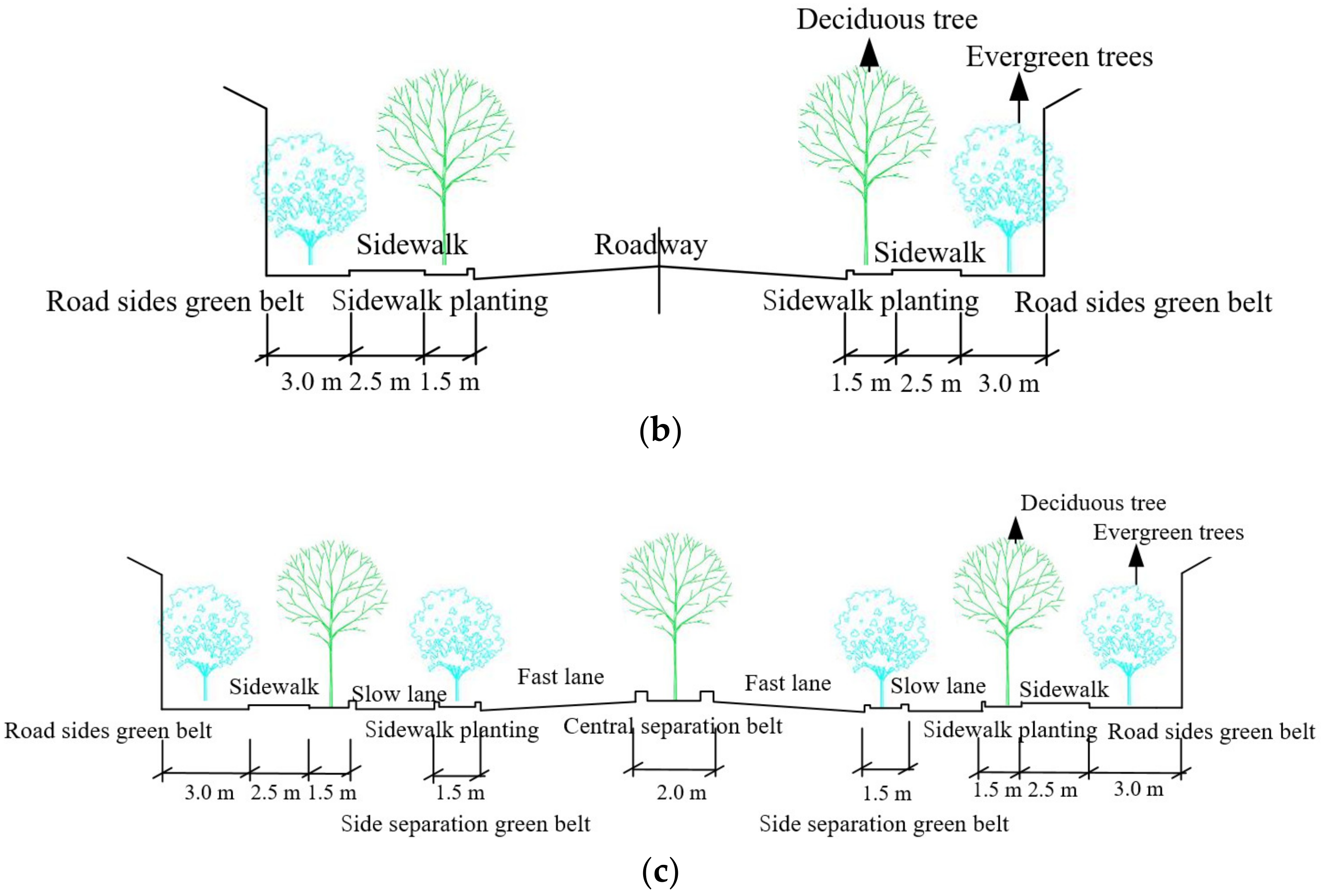
3.1. Urban Road Greening Arrangement Form and Basic Requirements

The layout of a road green-space belt on the section form of the urban road can be one-plate, two-plate, three-plate, or four-plate, corresponding to two belts, three belts, four belts, or five belts, respectively. The choice of an urban road greening arrangement form is closely related to road grades and red-line widths, which have different greening rate requirements for different road sections.

3.1.1. Arrangement Form of Urban Road Greening

Urban road grades are mainly categorized as expressways, trunk roads, secondary roads, and branch roads. The higher the road grade is, the more complicated the cross-sectional form. Three standard cross sections were screened out according to the Design Guidelines for Urban Greening Plant Configuration in Xi’an [45], as shown in Figure 1. The street trees are all calculated by assuming a single row because, according to the subsequent optimization model, the width will be adjusted to determine whether the rows should be single or multiple.

3.1.2. Basic Requirements for Urban Road Greening Design

According to the Design Guidelines for Urban Greening Plant Configuration in Xi’an [45], the Planning Standards for Integrated Urban Traffic System (GB/T 51328-2018) [46], the Design Specifications for Urban Road Greening (DB5301/T 20-2019) [47], and other specifications in China, explicit quantified requirements exist for designing urban road greening. Some of these, such as the greening requirements for different levels of roads, need to be added to the optimization model as constraints, as listed in

Table 5. Different Greening Rate Requirements for Different Roads.

Road Classification	Expressways		Trunk Roads			Secondary Roads	Branch Roads
Class Type	I	II	I	II	III		I	II
Number of two-way roads	4–8	4–8	6–8	4–6	4–6	2–4	2	-
Road red-line width	25–35	25–40	40–50	40–45	40–45	20–35	14–20	-
Greening rate requirement	≥30%		≥25%			≥20%	≥15%

.

3.2. Carbon Sequestration by Urban Road Greening

Traditional methods for calculating the amount of carbon sequestered by green-space plants include the biomass conversion factor method, biomass method, and assimilation method. The biomass method has high accuracy in its direct biomass measurement via standard wood analysis, and its anisotropic growth equation is convenient and fast. While the standard wood analysis method requires a large amount of workload and human and material resources, the anisotropic growth equation requires a large amount of actual measurement data. Meanwhile, the stage of growth of the tree species and regional differences should be considered. The biomass conversion factor method is relatively mature. However, parameters such as conversion factors need to be determined for different regions and species. The assimilation method has the following advantages: the carbon sequestration capacity of different plants can be evaluated, high carbon sink species can be screened, and the impact factors of plant photosynthesis can be analyzed. However, its carbon sink estimation involves uncertainties [48]. To facilitate the construction of optimization models, this research selects the assimilation method to calculate carbon sequestration.

3.2.1. Annual Carbon Sequestration per Unit of Plant

(1)

Carbon sequestration per unit leaf area

The daily net assimilation per unit leaf area is given in Equation (3):

$$p={\sum }_{i=0}^i[\frac{(p_{i+1}+p_i)}{2}\times (t_{i+1}-t_i)·\frac{3600}{1000}]$$

(3)

where p is the daily net assimilation per unit leaf area (mmol·m⁻²·s⁻¹); p_i is the instantaneous light and rate at the initial measurement point; p_i+1 is the instantaneous net photosynthetic rate at the next measurement point; t_i is the time at the current measurement point; and t_i+1 is the time at the next measurement point.

The amount of carbon sequestered per unit leaf area can be obtained from the photosynthetic reaction equation, as shown in Equation (4).

$$w_{c{o}_2}=p·44/1000$$

(4)

where $w_{c{o}_2}$ is the amount of carbon sequestered per unit leaf area (g·m⁻²·d⁻¹); 44 is the molar mass of CO₂.

(2)

Carbon sequestration per unit land area

The urban tree leaf area regression model obtained by Nowak (1994) [49] was used to calculate the leaf area of individual plants, as shown in Equation (5).

$$Y=\exp \left(0.6031+0.2375H+0.6906D-0.0123S_1\right)+0.1824$$

(5)

where Y is the total leaf area, m²; H is the height of the canopy, m; D is the diameter of the canopy, m; and S₁ = πD(H + D)/2.

The land area covered by the plant is the projected area of the plant canopy, S² = 1/4πD²(m²). Therefore, the leaf area index of a single plant is calculated as LAI = Y/S². The amount of carbon sequestered per unit land area (g·m⁻²·d⁻¹) is calculated from Equation (6).

$$Q_{{\mathrm{c}\mathrm{o}}_2}=LAI·w_{c{o}_2}$$

(6)

where LAI is the leaf area index of a single plant; $w_{c{o}_2}$ is the daily carbon sequestration per unit leaf area.

(3)

Calculation of daily carbon sequestration by individual plants

The daily carbon sequestration by individual plants is calculated from Equation (7).

$${M_{{\mathrm{c}\mathrm{o}}_2}=sQ}_{{\mathrm{c}\mathrm{o}}_2}$$

(7)

where s is the vertical projection area of the canopy of a single plant; M_co2 is the daily carbon sequestration of a single plant.

3.2.2. Annual Carbon Sequestration

Plant carbon sequestration is a cumulative indication parameter of the sum of carbon sequestration in all seasons of the year and thus can represent the total annual carbon sink capacity of the road network. According to the carbon sequestration ability in four seasons [50,51], peak vegetation carbon sink activity is mainly concentrated in summer, so summer is listed as the main season for vegetation carbon sequestration. Carbon sequestration is weakest in winter. Considering that evergreen vegetation forms a major part of urban road vegetation, the winter impact factor was defined as 1.0, and the impact coefficients of spring, summer, and autumn were chosen as 1.3, 1.6, and 1.3, respectively [52].

The annual carbon sequestration is calculated as shown in Equation (8).

$$W={\sum }_{i=1}^4{\sum }_{j=1}^N(R_{\mathrm{i}}·Q_{c{o}_2}·{\mathrm{S}}_j)\times 90$$

(8)

where W is the annual carbon sequestration; R is the seasonal influence factor; j is the plant species; Q_co2 is the daily carbon sequestration per unit area; and S_j is the vertical projection area of the tree canopy. In the calculation of S_j, the area of single trees and large shrub plants is calculated from the vertical projection area of the plant canopy, and the regular hedge area is calculated from the planting area.

Considering the road greening situation and native planting in Xi’an, acacia was selected as the tree type, zoysia as the shrub type, and mixed as the lawn type in this study. According to this investigation, the daily carbon sequestration amounts of the plants are 75.71 g/m²·d, 50.1 g/m²·d, and 6.17 g/m²·d, respectively. Therefore, the annual carbon sequestration amounts for trees, shrubs, and lawns were 35,432.28 g/m²·a, 23,446.8 g/m²·a, and 2887.56 g/m²·a, respectively.

3.3. Optimization Model Construction of Urban Road Green Belts under Carbon Peak Policy

The optimization model was constructed based on the above analysis to determine the width of different types of green belts. Regarding planting forms, trees are mostly planted in columns, shrubs in hedges, and mixed grasses in lawns and flower beds. Considering the characteristics of roads in Xi’an, the roads were classified according to their grades and red-line widths and divided into six categories. The road classification forms and green belt width symbols are presented in

Table 6. Road Type, Constraints and Symbols.

Road Type	Road Red-Line Width	Central Separation Belt and Side Separation Green Belt		Roadside Green Belt (Street Green)	Sidewalk Planting	Constraint Condition
		W111	W112	W12	W13	$0.3H_k$$\le \mathrm{W}111+\mathrm{W}112+\mathrm{W}12+\mathrm{W}13 \le { H}_{1h}-R_{1r}$ 1.5 ≤ W13 (The upper limit means that the width of the greenery cannot be greater than the difference between the width of the red line and the width of the road)
Expressways	80	Shrubs + dungarunga (giant cedar/sabina chinensis)	Shrubs + dungarunga	Trees, shrubs, and grasses (acacia + yew + mixed grass)	Trees and shrubs (acacia/ginkgo, Ligustrum macrophylla, etc.)
		W211	W212	W22	W23
Trunk roads	60	Shrubs + small trees (zoysia/large-leaved Maidenhair + small-leaved Maidenhair)	Shrubs + small trees	Trees, shrubs, and grasses (acacia + violet + mixed grass)	Trees + shrubs (acacia/ginkgo, chaste tree, etc.)	$2.8 < \mathrm{W}211; 1.5 \le \mathrm{W}23; 0.28H_k$$\le \mathrm{W}211+\mathrm{W}212+\mathrm{W}22+\mathrm{W}23 \le { H}_{2h}-R_{2r}$
		W311	W312	W32	W33
	50	Shrubs + small trees (zoysia/large-leaved Maidenhair + small-leaved Maidenhair)	Shrubs + small trees	Trees, shrubs, and grasses (acacia + violet + mixed grass)	Trees + shrubs (acacia/ginkgo, chaste tree, etc.)	$2.5 < \mathrm{W}311; 1.5 \le \mathrm{W}33; 0.25H_{k }$$\le \mathrm{W}311+\mathrm{W}312+\mathrm{W}32+\mathrm{W}33 \le H_{2h}-R_{2r}$
Secondary roads	30	--		W42	W43	$1.5 \le \mathrm{W}43; 0.2H_{k }$$\le \mathrm{W}42+\mathrm{W}43 \le { H}_{3h}-R_{3r}$
				Trees, shrubs, and grasses (acacia + violet + mixed grass)	Trees + shrubs (acacia/ginkgo, chaste tree, etc.)
	25	--		W52	W53	$1.5 \le \mathrm{W}53; 0.2H_{k }$$\le \mathrm{W}52+\mathrm{W}53 \le { H}_{3h}-R_{3r}$
				Trees, shrubs, and grasses (acacia + violet + mixed grass)	Trees + shrubs (acacia/ginkgo, chaste tree, etc.)
Branch roads	20	--		--	W63	$1.5 \le \mathrm{W}63; 0.15H_k$$\le \mathrm{W}63 \le H_{4h}-R_{4r}$
					Trees + shrubs (acacia/ginkgo, chaste tree, etc.)
Costs	Type	Trees/m2		Shrubs/m2	Ground cover plant/m2	Refer to the list of road greening projects and greening maintenance standards and charges of Xi’an City
	Plant cost	C11/one		C21/one	C31/m2
		200 1/3/3.5·200 = 19 (Yuan/m) (Average space per tree < 10 m2, i.e., average plant spacing ≈ 3.5 m)		60 1/2/1.5·60 = 20 (Yuan/m2)	10
	Maintenance costs (mainly contain pruning, fertilization, and pest control costs)	C12		C22	C32
		1 time/year 5 Yuan/m2		4 time/year 3 Yuan/m2	8 time/year 3.3 Yuan/m2

Note: H indicates the width of the red line, R indicates the width of the road.

.

Accordingly, an optimization model was constructed to minimize the total cost of greening, with the constraints that the carbon emissions should be less than carbon absorption while meeting the design requirements given in the specification. The optimization model is shown in Equation (9). The detail process can be found in Appendix A. Accordingly, under the goal of achieving a carbon peak, the optimization design can be performed for different road grades for greening in urban areas. The optimization model is a linear optimization model, which can be solved in Matlab.

$$\begin{gathered} \mathrm{Min}\mathrm{C}=\sum _{k=1}^3\sum _{n=1}^{t_{nk}}{l}_{nk}[\sum _{j=q\&g}\sum _{i=b\&h}{C}_{nji}·(w_{k11}+w_{k12}+w_{k2} \\ +w_{k3})+\sum _{i=b\&h}{C}_{nci}·w_{k3}] \\ +\sum _{k=4}^5\sum _{n=1}^{t_{nk}}{l}_{nk}[\sum _{j=q\&g}\sum _{i=b\&h}{C}_{nji}·(w_{k2} \\ +w_{k3})+\sum _{i=b\&h}{C}_{nci}·w_{k3}] \\ +\sum _{n=1}^{t_{n6}}{l}_{n6}[\sum _{j=q\&g}\sum _{i=b\&h}{C}_{nji}·w_{63}] \\ \mathrm{s}.\mathrm{t}. \sum _{k=1}^3\sum _{n=1}^{t_{nk}}{l}_{nk}[(\sum _{j=q\&g}{E}_{nj})·(w_{k11}+w_{k12}+w_{k2}+w_{k3}) \\ +E_{nc}·w_{k2}] \\ +\sum _{k=4}^5\sum _{n=1}^{t_{nk}}{l}_{nk}[(\sum _{j=q\&g}{E}_{nj})·(w_{k2}+w_{k3}) \\ +E_{nc}·w_{k2}] \\ +\sum _{n=1}^{t_{n6}}{l}_{n6}\left[\right(\sum _{j=q\&g}{E}_{nji})·w_{63}]\ge E_k \\ 0.3·H_{n1}\le w_{111}+w_{112}+w_{12}+w_{13}\le H_{n1}-R_{n1} \\ 1.5\le w_{13} \\ 0.28·H_{n2}\le w_{211}+w_{212}+w_{22}+w_{23}\le H_{n2}-R_{n2} \\ 2.5<w_{211} \\ 1.5\le w_{23} \\ 0.25·H_{n3}\le w_{311}+w_{312}+w_{32}+w_{33}\le H_{n3}-R_{n3} \\ 2.5<w_{311} \\ 1.5\le w_{33} \\ 0.20·H_{n4}\le w_{42}+w_{43}\le H_{n4}-R_{n4} \\ 1.5\le w_{43} \\ 0.20·H_{n5}\le w_{52}+w_{53}\le H_{n5}-R_{n5} \\ 1.5\le w_{53} \\ 0.15·H_{n6}\le w_{63}\le H_{n6}-R_{n6} \\ 1.5\le w_{63} \\ w\ge 0 \end{gathered}$$

(9)

In the above equation, k denotes the road type; t1-t6 indicates the number of different types of road strips; $l_{nk}$ represents the length of different types of roads for n roads; q, g, and c indicate trees, shrubs, and mixed grasses, respectively; $E_{nq}$ indicates the amount of carbon sequestered by trees in tons; $E_k$ is the amount of carbon to be sequestered; $H_{n1}$ indicates the red-line width for the type of road; $R_{n1}$ indicates the width of the road, which consists of motorized lanes, nonmotorized lanes, and sidewalks with widths of 3.25 m, 1 m and 2.5 m, respectively; w ≥ 0 indicates that the width of all green belts cannot be less than 0; b in $C_{nqb}$ indicates the cost of green tree species; and h in $C_{nqh}$ indicates the cost of green maintenance. The width symbols for each type of green belt are given in Table 6.

The upper and lower constraint limits for the optimization model are presented in

Table 7. Road Greening Width Constraints for Different Grades.

Road Type	Road Red-Line Width/m	Lower Limit of Constraint	Upper Limit of Constraint	Number of Motor Vehicle Lanes (Both Directions)
Expressways	80	24	47	6
Trunk roads	60	16.8	33.5	6
Trunk roads	50	12.5	30	4
Secondary roads	30	6	10	4
Secondary roads	25	5	11.5	2
Branch roads	20	3	6.5	2

Note: The width of the motor vehicle lane is 3.25 m, the width of the non-motor vehicle lane is 1 m, and the width of the sidewalk is 2.5 m.

.

4. Case Study

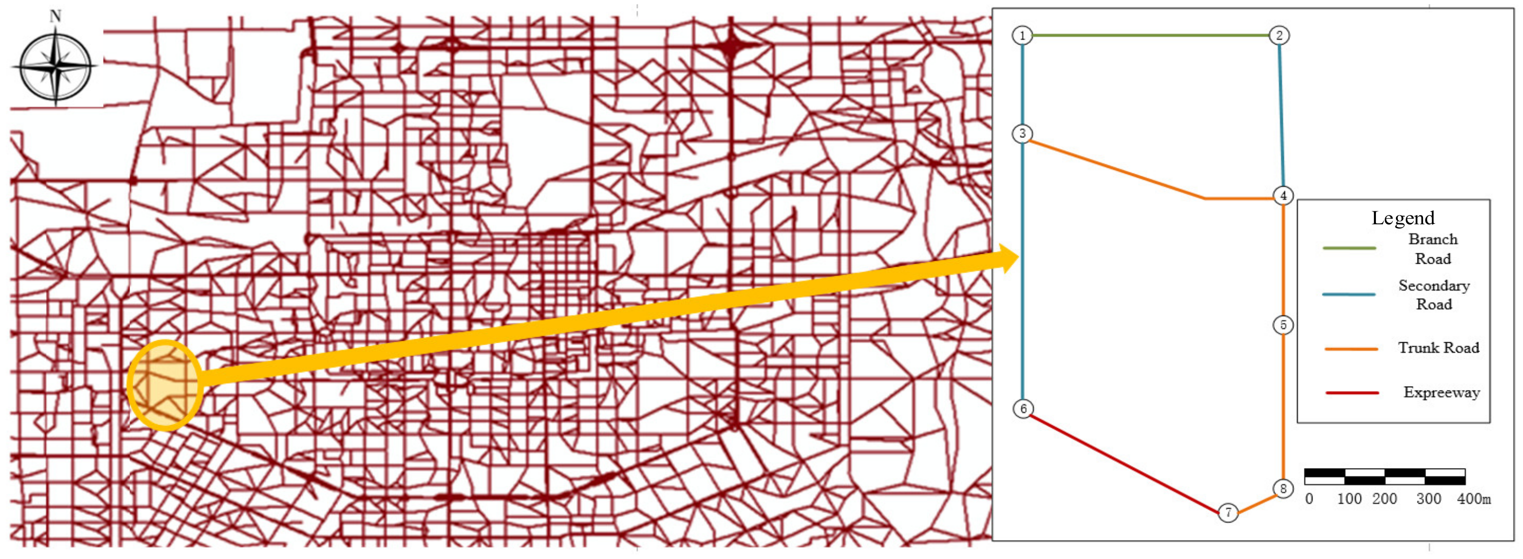
4.1. Road Network and Road Characteristics of Xi’an City

A small area of Qujiang was selected for a case study, as shown in Figure 2 (the connecting rod of the traffic cell on the right side of the line segment of the road network has be deleted). The road segment grade characteristics and road network traffic are presented in

Table 8. Characteristic of Roads.

Link	Road Grade	Length/m	AB Volume	BA Volume	Section Form	Current Red-Line Width/m
1–2	Branch road	589.25	57	31	One-carriageway, two-belt type	20
1–3	Secondary road	212.98	456	501	Three-carriageway, two-belt type	25
2–4	Secondary road	378.15	558.56	758.56	Three-carriageway, two-belt type	30
3–4	Trunk road	618.71	688	1146	Four-carriageway, five-belt type	50
3–6	Secondary road	680.76	308	410	Three-carriageway, two-belt type	25
4–5	Trunk road	296.29	1064	1504	Four-carriageway, five-belt type	60
5–8	Trunk road	383.3	1031	1172	Four-carriageway, five-belt type	60
8–7	Trunk road	131.9	1796	1302	Four-carriageway, five-belt type	60
6–7	Expressway	580.15	3408	4696	Four-carriageway, five-belt type	80

. The left figure is the road network of Xi’an City, which was obtained from the Urban Planning and Design Institute of Xi’an. The road network contains the characteristic data and traffic data of all road sections, including road type, road design speed, traffic speed, road traffic volume, road capacity, and the number of lanes, as well as other basic information. The figure on the right represents a small area of Qujiang, which is selected for this study. The four types of road are branch roads, secondary roads, trunk roads, and expressways. The road length, road traffic volume, road type, road grade, and road red line were extracted from a network database, and the section form was obtained via a field investigation. These data were used for analysis and determining the solution for the carbon emission and road greening optimization model in the case study.

First, the carbon emission of this area was calculated based on the ratio of the traffic volume of the region to the traffic volume of the whole of Xi’an City. The carbon emission of road traffic in Xi’an was 19,400 tons, and the proportion of traffic in the study area was 20,887.12 pcu/9,920,289.52 pcu = 0.0021. Therefore, the carbon emission of the road traffic in this area was 0.4074 Mt.

4.2. Optimization Results and Analysis of Results

From the optimization model in Section 3.3, the results with and without considering the roadside green belt width constraint are listed in

Table 9. Optimistic Results.

Without Considering the Roadside Green Belt Width Constraint
Road Type	Road Red-Line Width/m	Central Separation Belt/m	Side Separation Green Belt/m	Roadside Green Belt/m	Sidewalk Planting/m	Percentage of Greenery	Cost/Yuan
Expressway	80	9.25	7.96	0	7.55	0.31	8,026,348.2378
Trunk road	60	6.65	7.22	0	6.08	0.33
Trunk road	50	6.43	6.97	0	6.81	0.40
Secondary road	30	0	0	0	6.59	0.22
Secondary road	25	0	0	0	5.13	0.21
Trunk road	20	0	0	0	4.53	0.23
Considering the road-side green belt width constraint (only for the trunk roads and above-grade roads. The constraint is that roadside green belt width is greater than or equal to 3)
Road type	Road red-line width/m	Central separation belt/m	Side separation green belt/m	Roadside green belt/m	Sidewalk planting/m	Percentage of greenery	Cost/Yuan
Expressway	80	8.32	6.13	3	6.55	0.30	8,878,920.1033
Trunk road	60	5.70	5.0	3	6.35	0.33
Trunk road	50	4.67	5.77	3	6.95	0.41
Secondary road	30	0	0	0	6.28	0.21
Secondary road	25	0	0	0	5.37	0.21
Trunk road	20	0	0	0	3.88	0.19

.

Accordingly, the greening width ratio of the expressway, trunk road, secondary road, and branch road can be obtained from the optimization model. You [53] concluded that the green space area of the trunk road is 50% of the total road area, which is reasonable for a low-carbon trunk road cross-section design scheme. This study yielded green space area values of 0.33 and 0.4 for trunk roads are because the carbon emissions were shared by other road sections in the road network. The greening percentages of 30 and 31 for expressways are lower than those for trunk roads mainly because expressways are unsignalized continuous flow sections and, thus, have fewer carbon emissions than other road types due to frequent vehicle braking. A study [54] revealed that trunk roads have the highest CO₂ emission factor (298.61), which is greater than that of expressways (198.62). It also pointed out that trunk roads are the most important sources of carbon emissions in urban traffic, accounting for 41% of the total mileage, but their emission share of CO₂, CO, and HC is more than 50%, with a total share of 50.49%. In this study, trunk roads account for a large proportion of the length and traffic volume. Thus, the value is reasonable, and the method is feasible.

5. Conclusions

This paper quantitatively establishes the relationship between regional traffic carbon emissions and greening and determines the design parameters for urban road greening planning in the context of carbon peaking.

According to the scenario simulation result in the study, Xi’an can reach the carbon peak in the year 2025 with 18.045 Mt of carbon emissions under the given development scenario, and the traffic carbon emissions should be 2.71 Mt, with road traffic accounting for 1.94 Mt. An optimization model is constructed to minimize the cost of urban road greening based on this carbon peak development. The constraints requiring carbon absorption to exceed carbon emission and the greening width requirements given in the specification, which can effectively determine the optimal width of green belts for each type of urban roads of different grades and different red-line widths, are considered. According to the optimization model results, the greening ratio of the expressway is 0.30–0.31; the greening ratio of the main road that has a red-line width of 60 m, is 0.33; the greening ratio of the main road that has a red-line width of 50 m, is 0.40–0.41; the greening ratio of the secondary road, which has a red-line width of 30 m or 25 m, is 0.21–0.22; and the greening ratio of the branch road, which has a red-line width of 20 m, is 0.13. The greening ratio ranges from 0.13 to 0.23. In the actual planning, the width of each part and greening ratio can be finely adjusted according to the characteristics of the road and the surrounding environment, as well as aesthetic considerations, to meet the green and low-carbon as well as aesthetic targets.

In the future, more types of differentiated road red-line widths based on the road network of the whole of Xi’an City should be considered for a more in-depth study. This will result in a more reliable and accurate greening ratio and width distance of each part.

References

1. Axsen, J.; Plötz, P.; Wolinetz, M. Crafting strong, integrated policy mixes for deep CO2 mitigation in road transport. Nat. Clim. Change 2020, 10, 809–818. [Google Scholar]
2. Zhao, J.; Kou, L.; Wang, H.; He, X.; Xiong, Z.; Liu, C.; Cui, H. Carbon emission prediction model and analysis in the yellow river basin based on a machine learning Method. Sustainability 2022, 14, 6153. [Google Scholar]
3. González, L.; Perdiguero, J.; Sanz, A. Impact of public transport strikes on traffic and pollution in the city of Barcelona. Transp. Res. Part D Transp. Environ. 2021, 98, 102952. [Google Scholar]
4. Hao, J.; Chen, L.; Zhang, N. A statistical review of considerations on the implementation path of china’s “Double Carbon” goal. Sustainability 2022, 14, 11274. [Google Scholar]
5. Chen, L.; Msigwa, G.; Yang, M.Y.; Osman, A.I.; Fawzy, S.; Rooney, D.W.; Yap, P.S. Strategies to achieve a carbon neutral society: A review. Environ. Chem. Lett. 2022, 20, 2277–2310. [Google Scholar]
6. Ji, Y.B.B.; Dong, J.C.; Jiang, H.W.; Wang, G.; Fei, X. Research on carbon emission measurement of Shanghai expressway under the vision of peaking carbon emissions. Transp. Lett. 2023, 15, 765–779. [Google Scholar]
7. Gan, J.; Li, L.; Xiang, Q.; Ran, B. A Prediction Method of GHG Emissions for Urban Road Transportation Planning and Its Applications. Sustainability 2020, 12, 10251. [Google Scholar] [CrossRef]
8. Fang, G.C.; Wang, L.; Gao, Z.Y.; Chen, J.Y.; Tian, L.X. How to advance China’s carbon emission peak?—A comparative analysis of energy transition in China and the USA. Environ. Sci. Pollut. Res. 2022, 29, 71487–71501. [Google Scholar]
9. Tang, B.J.; Li, R.; Yu, B.Y.; An, R.Y.; Wei, Y.M. How to peak carbon emissions in China’s power sector: A regional perspective. Energy Policy 2018, 120, 365–381. [Google Scholar]
10. Lin, Z.S.; Wang, Y.T.; Ye, X.Y.; Wan, Y.X.; Lu, T.J.; Han, Y. Effects of Low-Carbon Visualizations in Landscape Design Based on Virtual Eye-Movement Behavior Preference. Land 2022, 11, 782. [Google Scholar]
11. Arshed, N.; Munir, M.; Iqbal, M. Sustainability assessment using STIRPAT approach to environmental quality: An extended panel data analysis. Environ. Sci. Pollut. Res. 2021, 28, 18163–18175. [Google Scholar] [CrossRef] [PubMed]
12. Gu, S.; Fu, B.; Thriveni, T.; Fujita, T.; Ahn, J.W. Coupled LMDI and system dynamics model for estimating urban CO2 emission mitigation potential in Shanghai, China. J. Clean. Prod. 2019, 240, 118034. [Google Scholar] [CrossRef]
13. Jahanger, A.; Usman, M.; Balsalobre-Lorente, D. Autocracy, democracy, globalization, and environmental pollution in developing world: Fresh evidence from STIRPAT model. J. Publ. Aff. 2021, 22, 2753. [Google Scholar] [CrossRef]
14. Ulucak, R.; Erdogan, F.; Bostanci, S.H. A STIRPAT-based investigation on the role of economic growth, urbanization, and energy consumption in shaping a sustainable environment in the mediterranean region. Environ. Sci. Pollut. Res. 2021, 28, 55290–55301. [Google Scholar] [CrossRef] [PubMed]
15. Wang, M.; Arshed, N.; Munir, M.; Rasool, S.F.; Lin, W. Investigation of the STIRPAT model of environmental quality: A case of nonlinear quantile panel data analysis. Environ. Dev. Sustain. 2021, 23, 12217–12232. [Google Scholar] [CrossRef]
16. Chen, H.; Zhang, X.; Wu, R.; Cai, T. Revisiting the environmental Kuznets curve for city-level CO2 emissions: Based on corrected NPP-VIIRS nighttime light data in China. J. Clean. Prod. 2020, 268, 121575. [Google Scholar] [CrossRef]
17. Li, Y.; Wang, Z.; Wei, Y. Pathways to progress sustainability: An accurate ecological footprint analysis and prediction for Shandong in China based on integration of STIRPAT model, PLS, and BPNN. Environ. Sci. Pollut. Res. 2021, 28, 54695–54718. [Google Scholar] [CrossRef]
18. Wang, P.; Wu, W.; Zhu, B.; Wei, Y. Examining the impact factors of energy-related CO2 emissions using the stirpat model in Guangdong Province, China. Appl. Energy 2013, 106, 65–71. [Google Scholar] [CrossRef]
19. Li, Z.H.; Murshed, M.; Yan, P. Driving force analysis and prediction of ecological footprint in urban agglomeration based on extended STIRPAT model and shared socioeconomic pathways (SSPs). J. Clean. Prod. 2023, 383, 135424. [Google Scholar] [CrossRef]
20. York, R.; Rosa, E.A.; Dietz, T. STIRPAT, IPAT and ImPACT: Analytic tools for unpacking the driving forces of environmental impacts. Ecol. Econ. 2003, 46, 351–365. [Google Scholar] [CrossRef]
21. Li, W.; An, C.L.; Lu, C. The Assessment Framework of Provincial Carbon Emission Peak Prediction in China: An Empirical Analysis of Hebei Province. Science of the Total Environment. Pol. J. Environ. Stud. 2019, 28, 3753–3765. [Google Scholar] [CrossRef]
22. Liu, X.D.; Wang, X.Q.; Meng, X.R. Carbon emission scenario prediction and peak path selection in China. Energies 2023, 16, 2276. [Google Scholar] [CrossRef]
23. Tian, S.; Xu, Y.; Wang, Q.S.; Zhang, Y.J.; Yuan, X.L.; Ma, Q.; Chen, L.P.; Ma, H.C.; Liu, J.X.; Liu, C.Q. Research on peak prediction of urban differentiated carbon emissions—A case study of Shandong Province, China. J. Clean. Prod. 2022, 374, 134050. [Google Scholar] [CrossRef]
24. Chai, Z.Y.; Yan, Y.B.; Simayi, Z.; Yang, S.T.; Abulimiti, M.; Wang, Y.Q. Carbon emissions index decomposition and carbon emissions prediction in Xinjiang from the perspective of population-related factors, based on the combination of STIRPAT model and neural network. Environ. Sci. Pollut. Res. 2022, 29, 31781–31796. [Google Scholar]
25. Li, C.; Zhang, Z.C.; Wang, L.P. Carbon peak forecast and low carbon policy choice of transportation industry in China: Scenario prediction based on STIRPAT model. Environ. Sci. Pollut. Res. 2023, 30, 63250–63271. [Google Scholar] [CrossRef]
26. Qin, J.C.; Tao, H.; Zhan, M.J.; Munir, Q.; Brindha, K.; Mu, G.J. Scenario analysis of carbon emissions in the energy base, Xinjiang autonomous region, China. Sustainability 2019, 11, 4220. [Google Scholar] [CrossRef]
27. Wang, Q.; Huang, J.J.; Zhou, H.; Sun, J.Q.; Yao, M. Carbon emission inversion model from provincial to municipal scale based on nighttime light remote sensing and improved STIRPAT. Sustainability 2022, 14, 6813. [Google Scholar] [CrossRef]
28. Chai, Z.; Simayi, Z.; Yang, Z.; Yang, S. Examining the driving factors of the direct carbon emissions of households in the Ebinur Lake Basin using the extended STIRPAT model. Sustainability 2021, 13, 1339. [Google Scholar] [CrossRef]
29. Li, W.J.; Kockelman, K.M. How does machine learning compare to conventional econometrics for transport data sets? A test of ML versus MLE. Growth and Change. Growth Change 2021, 53, 342–376. [Google Scholar] [CrossRef]
30. Xu, M.; Sbihi, H.; Pan, X.; Brauer, M. Local variation of PM2.5 and NO2 concentrations within metropolitan Beijing. Atmos. Environ. 2019, 200, 254–263. [Google Scholar] [CrossRef]
31. Selmi, W.; Weber, C.; Riviere, E.; Blond, N.; Mehdi, L.; Nowak, D. Air pollution removal by trees in public green spaces in Strasbourg city, France. Urban For. Urban For. Urban Green. 2016, 17, 192–201. [Google Scholar] [CrossRef]
32. Wang, J.; Feng, L.; Palmer, P.I.; Liu, Y.; Fang, S.X.; Bösch, H.; O’Dell, C.W.; Tang, X.P.; Yang, D.X.; Liu, L.X.; et al. Large chinese land carbon sink estimated from atmospheric carbon dioxide data. Nature 2020, 586, 720–723. [Google Scholar] [CrossRef] [PubMed]
33. Yadava, V.S.; Yadavb, S.S.; Gupta, S.R. Carbon sequestration potential and CO2 fluxes in a tropical forest ecosystem. Eco. Eng. 2022, 176, 106541. [Google Scholar] [CrossRef]
34. Zhao, X.C.; Li, F.S.; Yan, Y.Z.; Zhang, Q. Biodiversity in urban green space: A bibliometric review on the current research field and its prospects. Int. J. Environ. Res. Public Health 2022, 19, 12544. [Google Scholar] [CrossRef] [PubMed]
35. Romadhona, S.; Fitria, F.L.; Mandala, M. Carbon emission estimation model and correlation with green open space in Jember City Area. IOP Conf. Ser. Earth Environ. Sci. 2020, 485, 012116. [Google Scholar]
36. Carley, R.; Francisco, E.; Nicola, C.; Jorge, Z.C. Does “greening” of neotropical cities considerably mitigate carbon dioxide emissions? Thecase of Medellin, Colombia. Sustainability 2017, 9, 785. [Google Scholar]
37. Jung, T.Y.; Park, K.M. Analysis on preference for and importance of greening types of median strips for building low-carbon green network roads. J. Korea Landsc. Counc. 2020, 12, 140–153. [Google Scholar] [CrossRef]
38. Lin, S.; Sun, J.; Marinova, D.; Zhao, D. Effects of population and land urbanization on China’s environmental impact: Empirical analysis based on the extended STIRPAT model. Sustainability 2017, 9, 825. [Google Scholar] [CrossRef]
39. Wang, C.J.; Wen, B.; Wang, F.; Jin, L.X.; Ye, Y.Y. Factors driving energy-related carbon emissions in Xinjiang: Applying the extended STIRPAT model. Pol. J. Environ. Stud. 2017, 26, 1747–1755. [Google Scholar] [CrossRef]
40. Liu, D.N.; Xiao, B. Can China achieve its carbon emission peaking? A scenario analysis based on STIRPAT and system dynamics model. Ecol. Indic. 2018, 93, 647–657. [Google Scholar] [CrossRef]
41. Chen, W.; Yang, R. Evolving temporal-spatial trends, spatial association, and influencing factors of carbon emissions in mainland China: Empirical analysis based on provincial panel data from 2006 to 2015. Sustainability 2018, 10, 2809. [Google Scholar] [CrossRef]
42. Liu, R.J.; Ba, D.X. The relationship between urban compactness and urbanization level in capital cities of China. J. Nat. Resour. 2020, 35, 586–600. [Google Scholar]
43. Yang, S.X.; Ji, Y.; Zhang, D.; Fu, J. Equilibrium between road traffic congestion and low-carbon economy: A case study from Beijing, China. Sustainability 2019, 11, 219. [Google Scholar] [CrossRef]
44. Core Writing Team; Pachauri, R.K.; Meyer, L.A. (Eds.) IPCC, 2014: Climate Change 2014: Synthesis Report. Contribution of Working Groups I, II and III to the Fifth Assessment Report of the Intergovernmental Panel on Climate Change; IPCC: Geneva, Switzerland, 2014. [Google Scholar]
45. Xi‘an City Administration Bureau. Design Guidelines for Urban Greening Plant Configuration in Xi’an; Xi‘an City Administration Bureau: Xi’an, China, 2017.
46. GB/T 51328-2018; Planning Standards for Integrated Urban Traffic System. The Ministry of Housing and Urban-Rural Development of the People’s Republic of China: Beijing, China, 2018.
47. DB5301/T 20-2019; Design Specifications for Urban Road Greening. Kunming Market Supervision Administration: Kunming, China, 2019.
48. Ren, Y.; Wei, X.; Wei, X.H.; Pan, J.Z.; Xie, P.P.; Song, X.D.; Peng, D.; Zhao, J.Z. Relationship between vegetation carbon storage and urbanization: A case study of Xiamen, China. For. Ecol. Manag. 2011, 261, 1214–1223. [Google Scholar] [CrossRef]
49. Nowak, D.J. Air pollution removal by Chicago’s urban forest. In Chicago’s Urban Forest Ecosystem: Results of the Chicago Urban Forest Climate Project; McPherson, E.G., Nowak, D.J., Rowntree, R.A., Eds.; USDA Forest: Radnor, PA, USA, 1994; pp. 62–83. [Google Scholar]
50. Wang, J.; Xiang, Z.Y.; Wang, W.M.; Chang, W.J.; Wang, Y. Impacts of strengthened warming by urban heat island on carbon sequestration of urban ecosystems in a subtropical city of China. Urban Ecosyst. 2021, 24, 1165–1177. [Google Scholar] [CrossRef]
51. Geng, S.B.; Li, W.; Kang, T.T.; Shi, P.L.; Zhu, W.R. An integrated index based on climatic constraints and soil quality to simulate vegetation productivity patterns. Ecol. Indic. 2021, 129, 108015. [Google Scholar] [CrossRef]
52. Li, C.N. Analysis of carbon emission of vehicles and road area vegetation carbon sink of urban road. Master’s Thesis, Nanjing Forestry University, Nanjing, China, 2016. [Google Scholar]
53. You, X.B.; Xu, Z.B. Low carbon transportation: Seek zero carbon design for the transverse section of urban trunk roads. J. Gannan Teach. Coll. 2012, 33, 91–95. [Google Scholar]
54. Sun, D.; Zhang, Y.; Xue, R.; Zhang, Y. Modeling carbon emissions from urban traffic system using mobile monitoring. Sci. Total Environ. 2017, 599, 944–951. [Google Scholar] [CrossRef]
Figure 1. Road Cross-Section Form. (a) One-carriageway, two-belt type (no roadside green belt). (b) One-carriageway, two-belt type (with roadside green belt). (c) Four-carriageway, five-belt type (with roadside green belt).
Sustainability 15 13140 g001aSustainability 15 13140 g001b
Figure 2. Road Network, Qujiang Area in Xi’an, Shaanxi.
Sustainability 15 13140 g002