Abstract
A vehicle exposed to flooding may lose its stability and wash away resulting in potential injuries and fatalities. Traffic disruption, infrastructure damage, and economic losses are also additional effects of the washed vehicles. Therefore, understanding the responses of passenger vehicles during flood events is of the utmost importance to reduce flood risks and develop accurate safety guidelines. Previously, flooded vehicle stability was investigated experimentally, theoretically, and numerically. However, numerical investigations are insufficient, of which only a few studies have been published since 1967. Furthermore, coupled motion simulations have not been employed to investigate the hydrodynamic forces on flooded vehicles. In this paper, a numerical framework was proposed to assess the response of a full-scale medium-size passenger vehicle exposed to floodwaters through three-dimensional computational fluid dynamic modelling. The vehicle was simulated under subcritical and supercritical flows with the Froude number ranging between 0.09 and 2.46. The results showed that the vehicle experienced the floating instability mode once the flow depth reached 0.38 m, while the sliding instability mode was observed once the threshold function exceeded 0.36 m2/s. In terms of hydrodynamic forces, it was noticed that the drag force decreased with the increment of the Froude number and flow velocity. On the other hand, the fraction and buoyancy forces are mainly governed by the flow depth at the vehicle vicinity. The drag coefficient was noticed to be less than 1 for supercritical flows and more than 1 for subcritical flows. The numerical results obtained through the framework introduced in this study demonstrate favorable agreement with three different previously published experimental outcomes.
1. Introduction
At several locations, roads and watercourses commonly intersect in their layout. These crossings happen through bridges or drainage works and fords. During rainy seasons, watercourses along the roadway may flood, resulting in significant disruption for the traffic movement [1]. Attempting to cross the flooded roadways in these circumstances can be extremely dangerous [2,3]. According to the statistics, many drivers and passengers are washed away in their vehicles every year when attempting to cross flooded roadways, and many of them drown [4,5,6]. Enriquez-de-Salamanca (2020) [1] investigated vehicle-related fatalities in Spain between 2008 and 2018. It was found that a total of 125 accidents were reported for people crossing flooded roadways, of which 33 accidents were reported with fatalities. A total of 200 persons were consequently involved in these accidents; 45 of them died, 137 needed rescue, and 18 managed to survive on their own [1]. Ahmed et al. (2020) [7] analyzed vehicle-related flood fatalities in Australia over the period 2001 to 2017. According to their results, it was noticed that among the 74 flood-related vehicle incidents, 96 people died [7]. Diakakis and Deligiannakis (2013) [4] conducted an analytical study to understand the relationship between floods and vehicle-related fatalities between 1970 and 2010 in Greece. They reported that among the 37 flood events, a total of 60 deaths were recorded. In this context, the danger of crossing flooded roadways and the need for proper safety guidelines are made clear.
Essentially, moving water generates different hydrodynamic (HD) forces on the objects that may exist along the flow direction. For the flooded stationary vehicles, the hydrodynamic forces are the drag (FD) and buoyancy forces (FV) [8,9]. Vehicles resist these hydrodynamic forces through the vehicle weight (FW) and the frictional force (FR) between the tires and ground surface [10]. Due to the generated HD forces, vehicles may lose their stability in two common ways, namely (i) sliding instability mode which commonly occurs when the drag force exceeds the frictional force, and (ii) floating instability mode which mainly occurs once the buoyancy force exceeds the vehicle weight [11,12]. The flow velocity and water depth at the vehicle vicinity are the main flow parameters that have the highest effect on the flooded vehicle’s stability [13,14]. On the other hand, vehicle characteristics such as weight, dimensions, ground clearance, and aerodynamic shape play main roles in increasing or decreasing the stability limits [15]. Developing proper safety guidelines and strategies while maintaining or enhancing the overall sustainability of communities and ecosystems is required to minimize flood risks. Sustainable safety guidelines for flooded vehicles are a part of the integrated flood management (IFM) plan which also requires engaging and educating communities on the potential risks of driving through flooded roadways, evacuation plans, and preparedness measures.
Between 1967 and 2021, several experimental studies were conducted to investigate the vehicle response inside floodwaters, while few numerical studies were published in this regard [16]. The earliest numerical simulation on vehicle instability was conducted in 2011 by Xia et al. (2011) [17]. The numerical runs were designed to investigate the stability of people and vehicles exposed to flash flood events. The study was performed by using an existing 2D hydrodynamic model which employs the finite volume method (FVM) based on an unstructured triangular mesh and depth-averaged 2D shallow water equation to solve the fluid flow numerically. A hazard degree (HD) expression was introduced and used to quantify the corresponding degree of hazard. Based on the HD value, vehicles were considered to be safe if the HD = 0, while vehicles were considered to be unsafe if the HD approached 1.0. The hydrodynamic model was validated by simulating three actual flood disasters, including the Glasgow, Boscastle, and Malpasset flood events. The obtained numerical results were in line with the actual flood scenarios [17].
In 2015, Arrighi et al. (2015) [18] studied the instability scenarios of a flooded vehicle using a numerical approach by employing the computational fluid dynamics (CFD) toolbox in OpenFOAM. For the purpose of numerical simulation, a Ford Focus model was chosen to represent the class medium city car which was previously tested experimentally by Shu et al. (2011) [14]. Two different flow orientations were simulated, namely 0° (the front end of the car faces the incoming flow) and 360° (the rear end of the car faces the incoming flow). Hydrodynamic forces, drag, and left confections were computed at each time step. From this numerical study, a mobility parameter called θv was presented to describe vehicle instability modes as a function of the Froude number. The numerical model outcomes were compared with Shu et al.’s (2011) [14] experimental outcomes, and a strong correlation between the two studies was found. Albano et al. (2016) [19] performed three-dimensional (3D) numerical modelling to study the groynes effects on the washed debris including vehicles during flood events in urban areas. The numerical runs were performed by using the Smoothed Particle Hydrodynamics (SPH) model which was reported by Amicarelli et al. (2015) [20]. The findings demonstrated that various groynes geometrical shapes have various effects on the washed bodies. The results of the numerical simulation were validated using experimental tests with the same setup and boundary conditions of the numerical simulation and both experimental and numerical results were properly aligned with each other.
In 2018, another numerical assessment of flooded vehicle instability was carried out by Gomez et al. (2018) [21] and Gomariz et al. (2019) [22]. A 3D commercial software was used to perform the numerical runs, namely FLOW-3D which employed the finite volume method (FVM) to solve the turbulent models as well as the flow governing equations [23]. One vehicle model, namely the Mercedes Class C, was selected to be simulated. The vehicle model was placed perpendicular to the flow direction at which the vehicle’s longitudinal side was facing the incoming flow. The hydrodynamic forces were obtained in all directions, and it was concluded that the vehicle slides once the drag force exceeds the frictional force. The floating instability mode occurs when the buoyancy force exceeds the vehicle weight. Numerical and previously published experimental [13] findings were compared, and it was found that the two results were in good accord. Recently, in 2020, Al-Qadami et al. (2021) [24] carried out a numerical investigation to study the floating instability of a small-size passenger vehicle using six degrees of freedom and coupled motion numerical simulation. However, sliding instability and horizontal and vertical forces were not considered and measured. The results revealed that the vehicle floated at 0.38 m water depth and 9.2 KN buoyancy force. Numerical results were validated with experimental results and good agreement was noticed.
Based on the above discussion, it can be concluded that the previously published numerical runs either did not focus on specific vehicle models as such the studies that were reported by Xia et al. (2011) [17] and Albano et al. (2016) [19], or did not employ the fully coupled numerical simulation, i.e., the vehicle models were simulated as a fixed object [18,22,23]. Al-Qadami et al. (2021) [24] adopted the fully coupled and six-degrees-of-freedom numerical simulation; however, both studies focused only on the floating instability mode, while the sliding instability mode and hydrodynamic forces on static vehicles were not covered. In this study, a numerical framework is proposed to investigate the hydrodynamic forces acting on a full-scale static flooded vehicle under subcritical and supercritical flows. The science of computational fluid dynamics (CFD) coupled with six degrees of freedom and coupled motion simulation tools were employed to conduct the numerical runs. This paper firstly presents a general description of the governing equations that were used to solve the 3D fluid flow and turbulence models. Then, meshing and geometry creation are explained including the mesh size selection criteria, mesh block arrangement, and mesh-independent study. Next, the numerical setup is discussed in detail including boundary conditions, material properties, and initial conditions. Later, the results are presented and discussed, and a comparison between the obtained results and previously published works is performed. Finally, some conclusions are presented regarding the proposed methodology at the end of this paper.
2. Methodology
In this study, a computational fluid dynamic (CFD) software, namely FLOW-3D version 11.2, which employs the finite volume method (FVM) and turbulence models to solve the continuity and Navier Stoke’s equations [25] was chosen to perform the numerical simulation. All numerical runs in this study were conducted under coupled motion and six degrees of freedom conditions. Such a setup allows us to detect the center of mass (COM) of the vehicle at every time step and visualizes whether the vehicle is stable or not. One vehicle model called Peruodu Viva was chosen to represent a medium-sized Malaysian passenger vehicle. The vehicle model was tested under different scenarios of flow depths and velocities with a Froude number ranging between 0.09 and 2.46.
2.1. Governing Equations
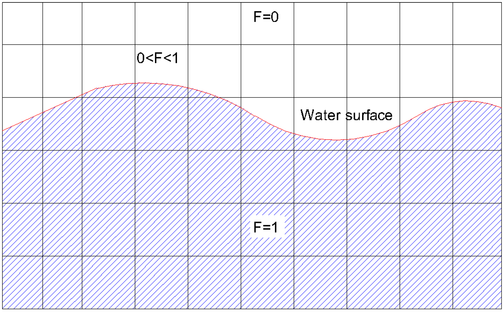
Among the numerical setups, mass continuity (Equation (1)) and momentum equations (Equations (2)–(4)) at the Cartesian coordinate system were selected to solve fluid flows in 3D form [26]. The k-Ɛ turbulence model with a no-slip wall shear boundary condition was selected to solve the turbulence flow. The k-Ɛ turbulence model is counted as an advanced and more popular model to solve turbulence flow and it can provide reasonable and accurate approximations for a variety of flows [27,28]. The two transport equations of the k-ε turbulence model are (i) the turbulent kinetic energy kT (Equation (5)) and (ii) its dissipation εT (Equation (6)) [26]. To detect vehicle movement and allow for coupled modelling conditions, the general moving object model (GMO) was enabled. The collision model was enabled as well to solve the rigid body dynamic equations. FLOW3D was specifically designed to handle scenarios involving free surfaces, and it incorporates an exclusive interface-tracking and free-surface-advection technique known as TruVOF which adopts a mixed Lagrangian-Eulerian approach. This method aims to address challenges inherent in standard volume of fluid (VOF) advection approaches such as over-filling or over-emptying computation cells when volume fluxes are significant in all directions and the time step is close to the local Courant stability limit [29]. TruVOF reportedly reduces the necessity for many cells in the vicinity of the free surface, potentially leading to computational time savings in comparison to other computational fluid dynamics (CFD) software like CFX (https://www.ansys.com/) [30]. The volume of fluid (TruVOF) function F (x, y, z) ranging between 0 and 1, at which F = 1 refers to the cells full of fluid, F = 0 refers to the empty cells, and 0 < F < 1 refers to cells partially full of fluid as shown in Figure 1 [23]:
where VF is the fractional volume open to flow, ρ is the fluid density, t is the time, (u, v, w) are the velocity components in the coordinate directions (x, y, z), RSOR is the density source term, (Ax, Ay, Az) are the fractional areas open to flow in the (x, y, z) directions, respectively, (Gx, Gy, Gz) are the body accelerations, (fx, fy, fz) are vicious accelerations, P is the pressure, GT is the buoyancy production term, PT is the turbulent kinetic energy production, DiffKT is the diffusion term, and CDIS1, CDIS2, and CDIS3 are dimensionless user-adjustable parameters and have defaults of 1.44, 1.92, and 0.2, respectively.
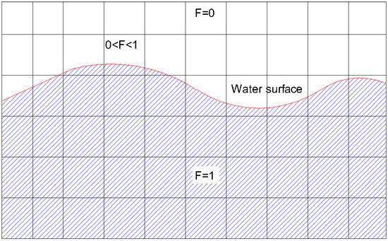
Figure 1.
2D view illustrates the free surface integrated via the volume of fluid function [23].
Figure 2 shows the block diagram of the computational process in FLOW-3D that was adopted in this study. The process starts by defining the initial and boundary conditions, and then the algorithm starts to solve the velocity and pressure fields. Next, once these parameters begin to approach convergence, the supplementary calculations begin. Later, the next cycle of calculations begins if the simulation time does not approach the finish time, but if the simulation timing reaches the finish time, then the post-process will be initiated, and the simulation will be terminated.
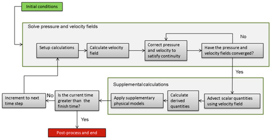
Figure 2.
Computational procedure block diagram in FLOW-3D.
2.2. Meshing and Geometry
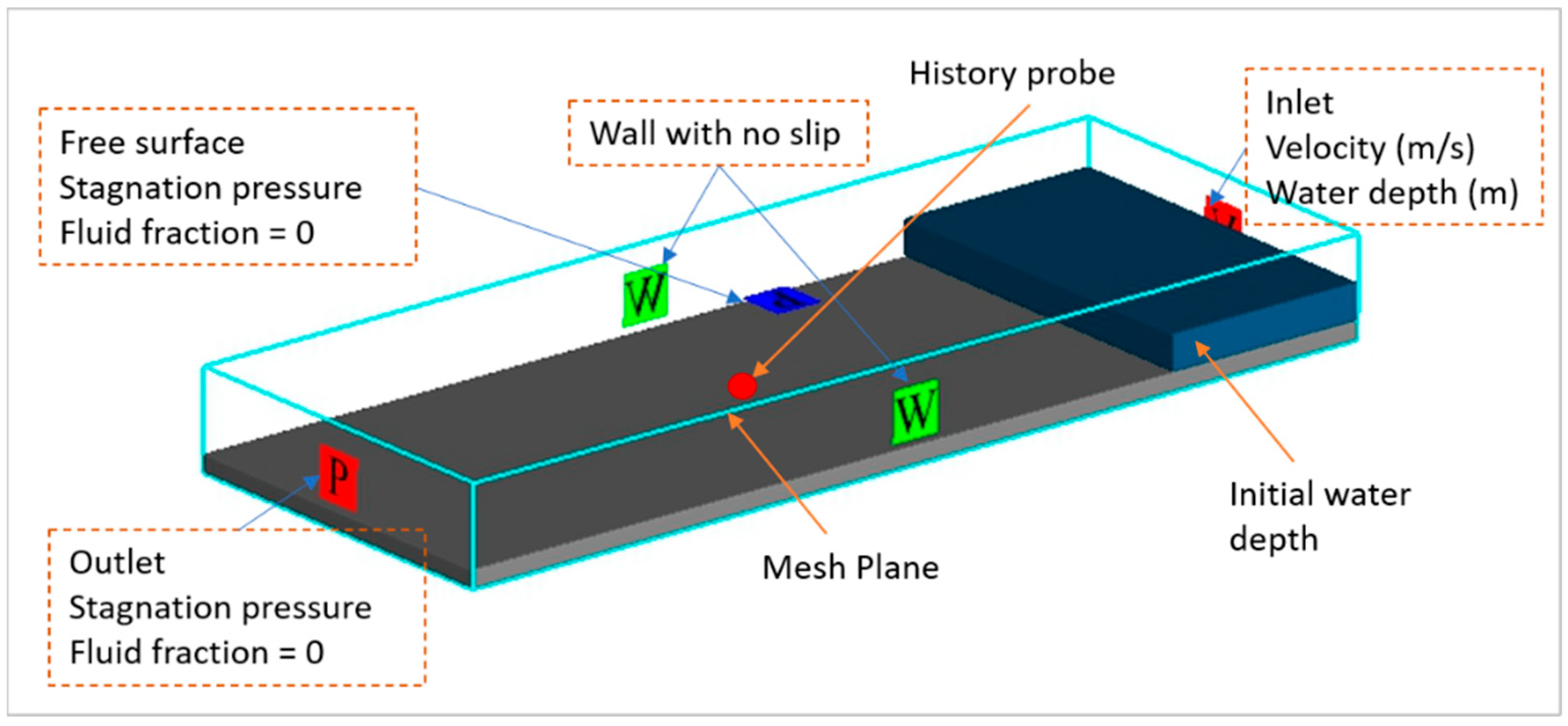
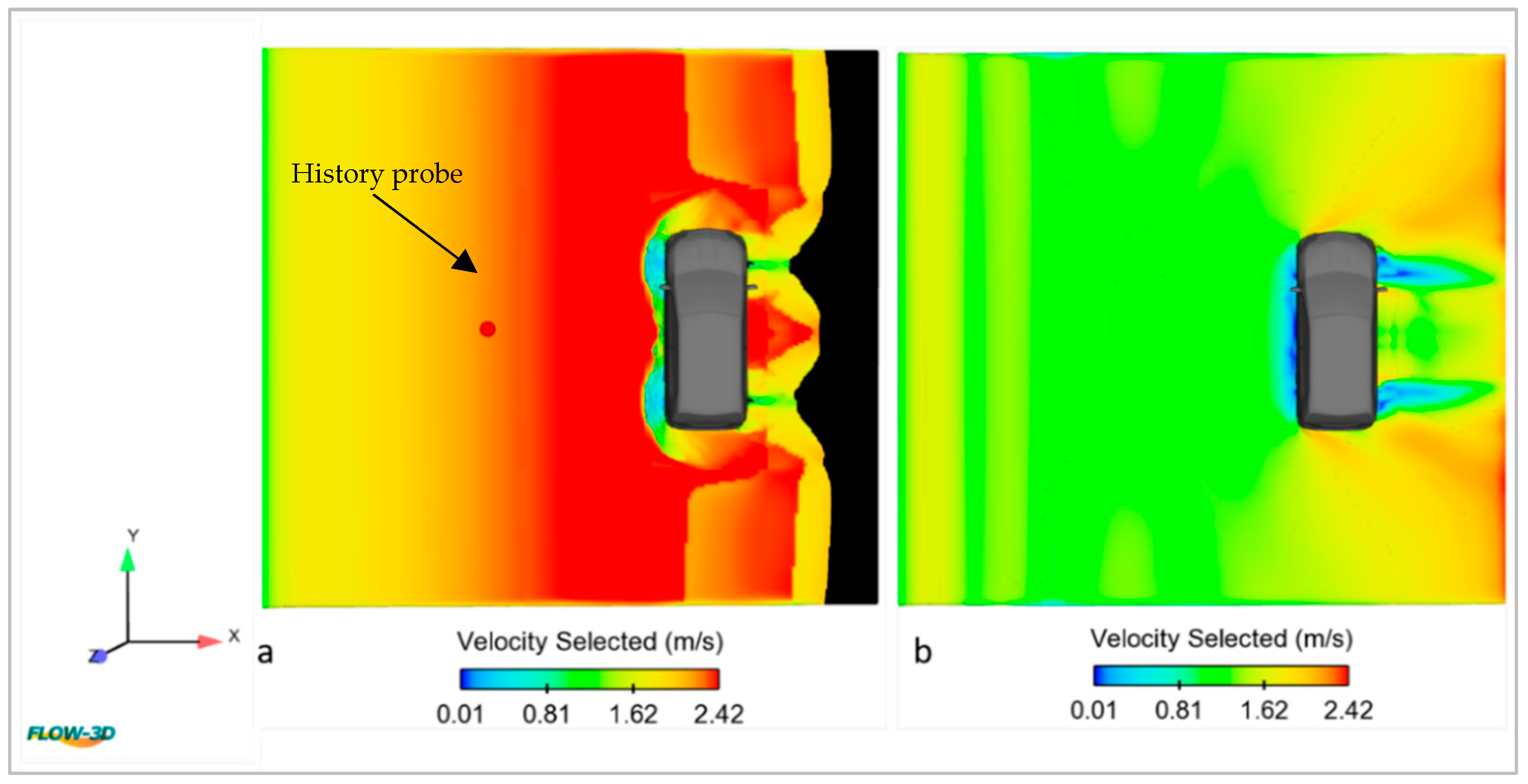
FLOW-3D uses orthogonal mesh, and it can be in Cartesian or cylindrical coordinates. In this study, a uniform orthogonal mesh with the Cartesian coordinate system was used. The mesh’s cell size was selected based on three criteria, namely (i) geometry accuracy after applying Fractional Area/Volume Obstacle Representation (FAVOR) solver, (ii) required time for simulation (system capabilities), and (iii) quality of the results (mesh-independent study). The mesh-independent study was performed by testing a total of four mesh blocks with cell sizes of 0.1, 0.075, 0.05, and 0.025 m. The setups of the numerical modelling for the purpose of mesh-independent study are shown in Figure 3. The inlet was defined with velocity and depth, while the outlet was defined as a free outlet with atmospheric pressure. One fluid history probe was used to measure the values of the flow parameters including flow velocity and Froude number.
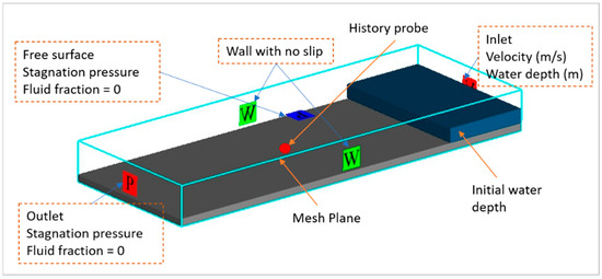
Figure 3.
Mesh-independent study numerical setup.
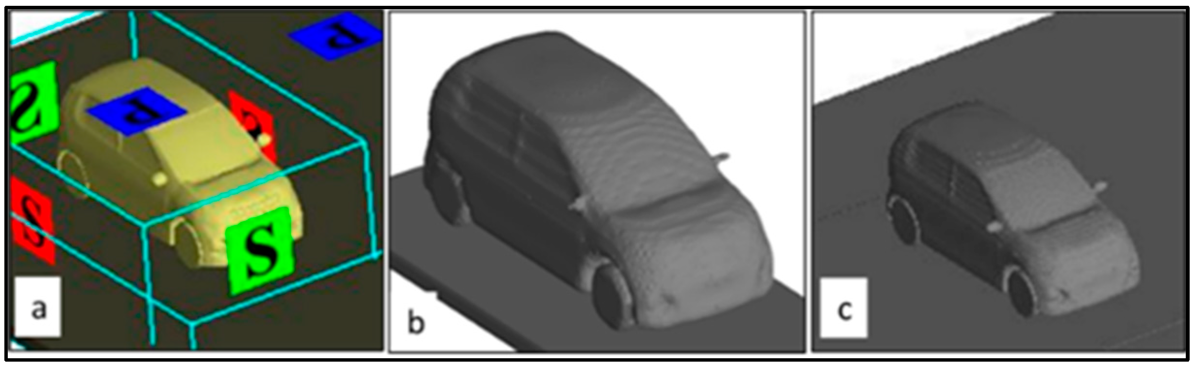
Table 1 shows the average values of the Froude number and flow velocity at a steady state for the different mesh sizes. It can be seen that the mesh blocks with cell sizes of 0.100 m and 0.075 m provided readings with a noticeable difference when compared with other mesh cell sizes (0.05 m and 0.025 m). The Froude number and flow velocity values obtained from the mesh blocks with cell sizes of 0.05 m and 0.025 m are very close with an average percentage difference of 1%. Therefore, by considering the computational time and system capabilities, a mesh block with a cell size of 0.05 m was chosen to capture the fluid domain. Later, the mesh quality in terms of its accuracy in capturing the vehicle geometry details was checked by running the FAVOR solver [26] which is available in FLOW-3D. Figure 4a,b shows a comparison between the meshed and favorized geometries using a 0.05 m cell size which was generated from the mesh-independent study. It was found that the mesh block with a cell size of 0.05 m could not capture the car model details accurately. Therefore, a nested mesh block was defined with a cell size of 0.025 m to only capture the vehicle domain. Figure 4b,c shows a comparison between the favorized geometries using 0.05 m and 0.025 m cell sizes, respectively.

Table 1.
Average Froude number values at different cell sizes at steady state.

Figure 4.
(a) Meshed geometry, (b) favorized geometry (0.05 m cell size), and (c) favorized geometry (0.025 m cell size).
The vehicle’s 3D geometry model was created by SolidWorks software 2016 with the same dimensions and shape design as the real car’s geometry. The geometry was then converted to stereolithography (STL) file format and imported into FLOW-3D. Figure 5 shows the 3D geometry model which was created for numerical simulation purposes and the real car model. The road 3D geometry model was created using FLOW-3D software as a rectangle plate with dimensions of 10 m width, 12 m length, and 0.22 m height. Later, the vehicle model was placed on the surface of the created road plate.
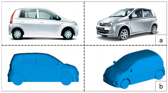
Figure 5.
Comparison between: (a) the real vehicle, and (b) the generated 3D model.
2.3. Numerical Setup
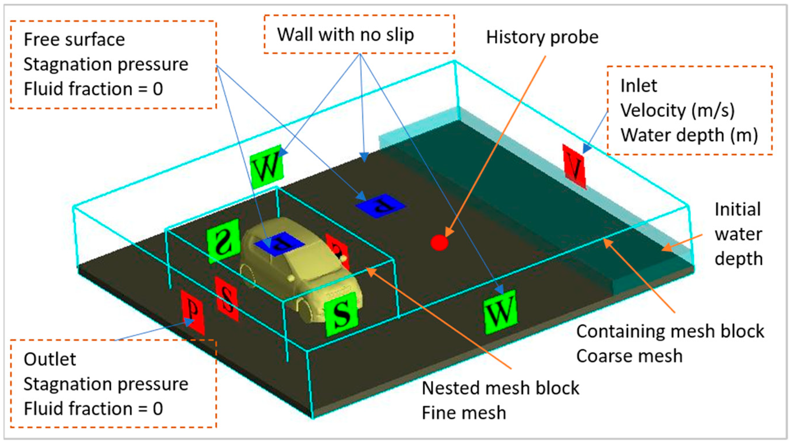
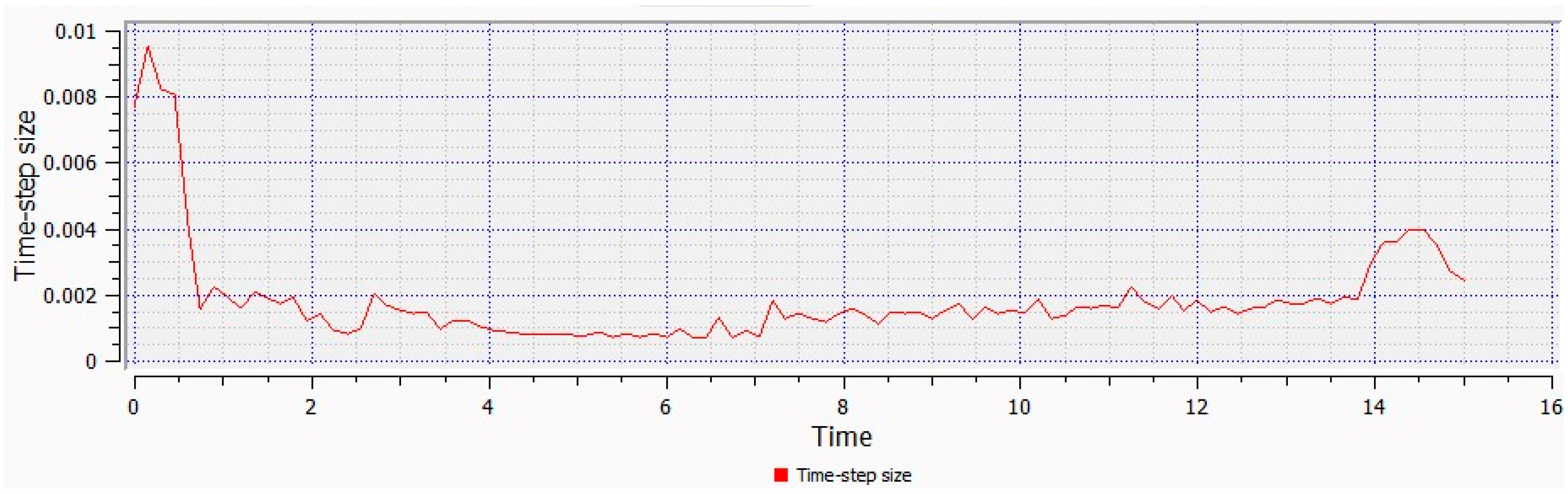
The numerical simulation process was started by defining the general parameters and physics models discussed in Section 2.1. Later, the 3D geometry vehicle model was inserted into the FLOW-3D software interface as an STL file, then the 3D geometry model of the road was generated using the tools incorporated in FLOW-3D. A static friction of 0.30 and a coefficient of restitution of 1.0 were used to define the interaction between the road surface and the vehicle tires. One history probe was located 3 m ahead of the vehicle to record the flow parameters (flow depth, flow velocity, and Froude number) as shown in Figure 6 and Figure 7. For each run, the time of simulation was chosen to be 16 s. This time was adopted based on two criteria, firstly to ensure that the vehicle does not drag outside the computational domain boundary for unstable cases, and secondly to ensure that the flow properties at the history probe reach a steady state for stable cases. The time step is a critical parameter that affects the stability, accuracy, and computational efficiency of simulations. FLOW-3D incorporates an inherent stability control feature, which automatically adapts the time step to ensure the solver operates within stability thresholds. While users can manually designate the time step size, superior and more stable outcomes have been observed when allowing the solver to determine the time step size during each iteration [30]. The average time step that was used by the FLOW-3D solver was found to be 0.001 s, as shown in Figure 8. By using Equation (7), the Courant–Friedrichs–Lewy (CFL) number that corresponds to the average time step can be calculated, and the value was found to be 1.2:
where, ux is the maximum expected velocity in the x-direction, uy is the maximum expected velocity in the y-direction, Δt is the time step, and Δx and Δy are the grid spacings in the x-direction and y-direction, respectively.

Figure 6.
Numerical setup for subcritical flow runs.

Figure 7.
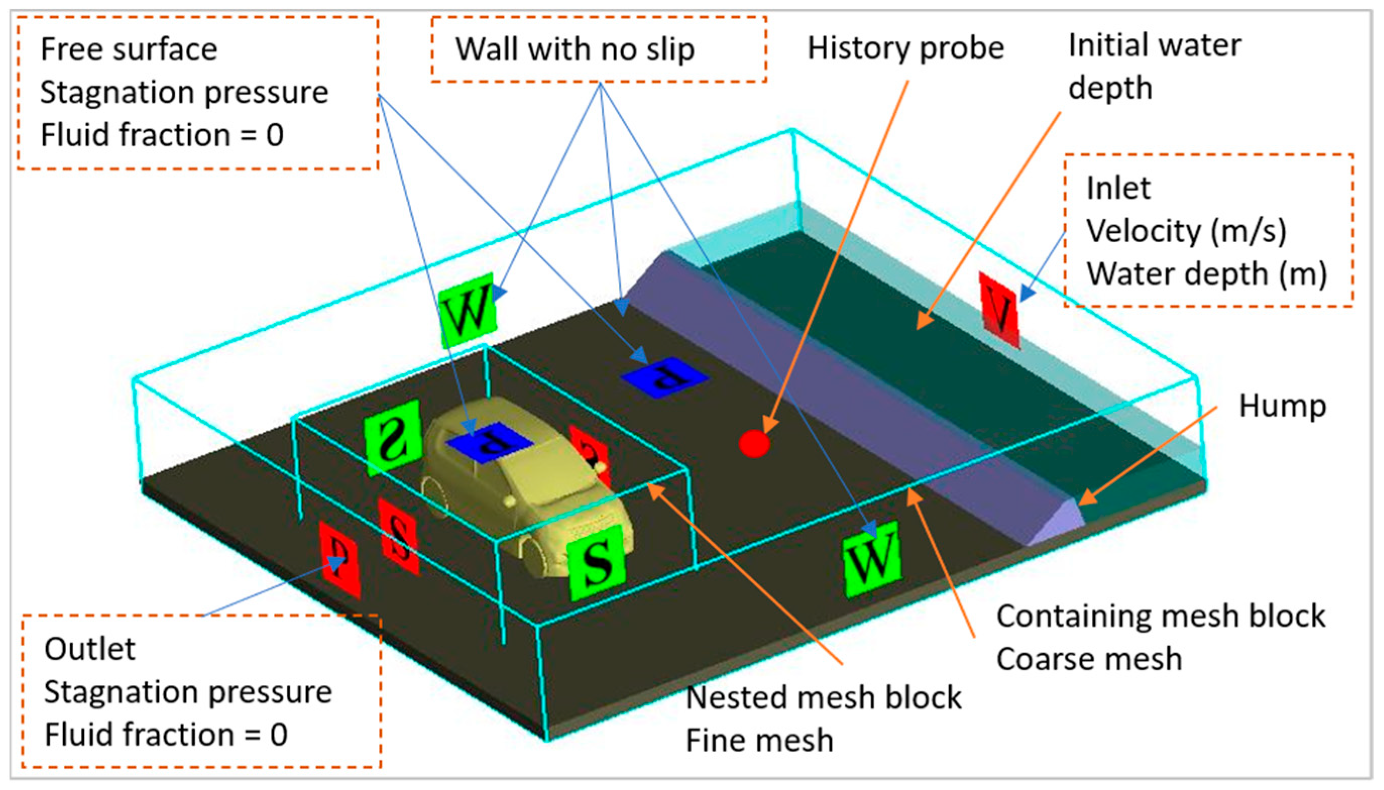
Numerical setup for supercritical flow runs.
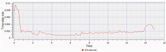
Figure 8.
The time step size the FLOW3D solver used on the selected mesh size.
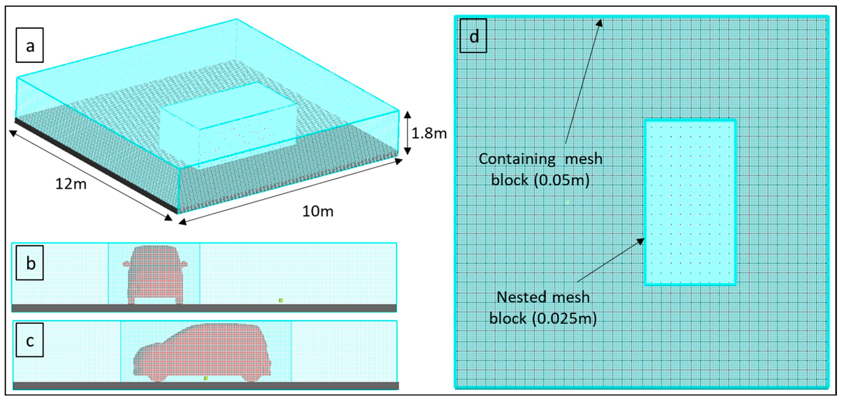
Two mesh blocks were used, namely (i) containing mesh block and (ii) nested mesh block, as shown in Figure 9. The containing mesh block captured both the fluid and geometry domains with a cell size of 0.05 m in x-, y-, and z-directions. The boundary conditions of the containing mesh block were defined for each face as follows: (i) top was defined as a free surface with stagnation pressure and zero fluid fraction, (ii) both sides and bottom faces were defined as walls with no slip, (iii) inlet face was defined with flow velocity and water depth, and (v) outlet face was defined as a pressure outlet with atmospheric pressure and zero fluid fraction. The nested mesh block was located inside the containing mesh block with a cell size of 0.025 m. A smaller cell size was chosen for the nested mesh block to capture all vehicle details, as discussed in Section 2.2. All sides of the nested mesh block were defined as symmetry except the top face, which was defined as a free surface with stagnation pressure and zero fluid fraction. The computational domain has dimensions of 10 m in width, 12 m in length, and 1.8 m in height as shown in Figure 9. The blockage ratio (BR) which refers to the ratio of the projected side area of the vehicle to the frontal area of the domain was calculated using Equation (8) [31] and it was found to be 0.22.
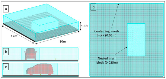
Figure 9.
Mesh blocks, (a) isometric view, (b) side view, (c) front view, and (d) top view.
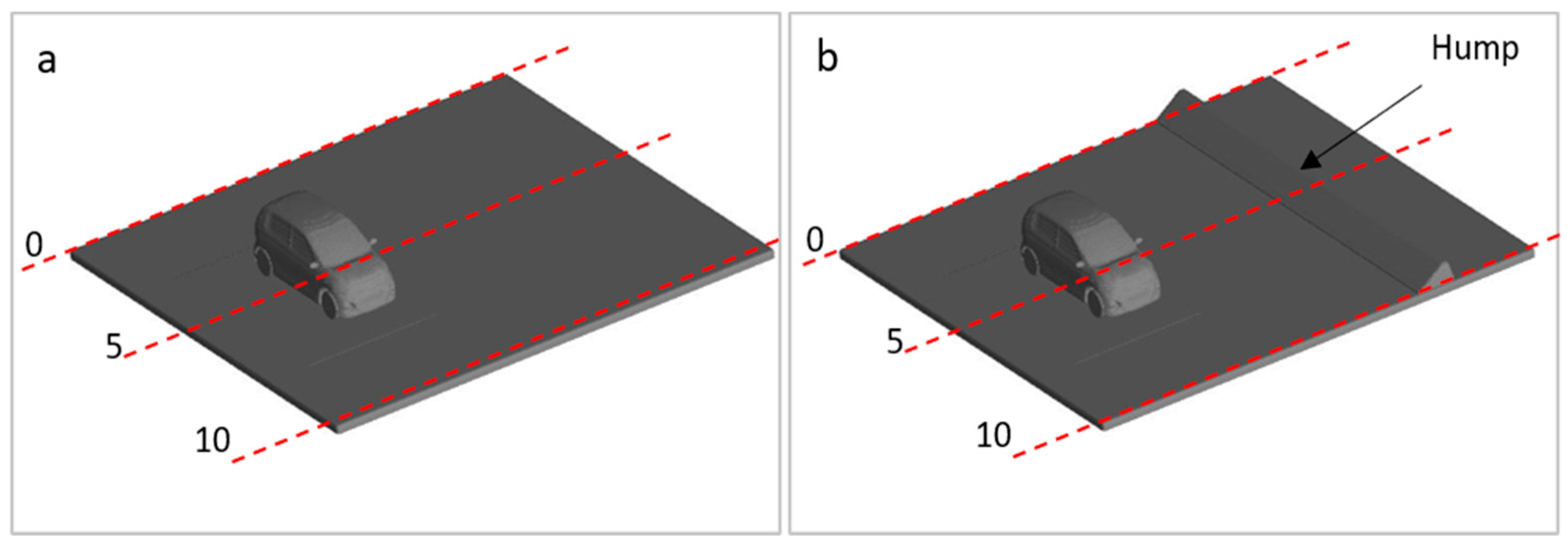
A total of 3,419,280 cells were accounted for both in containing and nested mesh blocks. It is worth mentioning that the numerical runs were performed in a workstation PC with 16GB RAM and 64bit CPU at which the time taken by the PC to complete one numerical run successfully ranged between 3 and 4 days. Figure 6 shows the numerical set-up and boundary conditions that were used to investigate the different hydrodynamic forces on a flooded vehicle under subcritical flows. On the other hand, a hump was designed and placed at the inlet side to simulate the supercritical flows as shown in Figure 7. Later, different flow velocities and depths were generated through the inlet boundary. As previously discussed, the mesh quality for each setup was checked before running the numerical modelling using the FAVOR solver. Figure 10 shows the output of the Favor solver for the whole solid domain (road and vehicle models). A total of 14 numerical runs were carried out to investigate the different hydrodynamic forces on the critical vehicle orientation 90° [16] (i.e., the vehicle’s longitudinal side was facing the incoming flow) under subcritical and supercritical flows. Table 2 provides a summary of the hydraulic parameters (velocity, depth, and Froude number) measured 3.0 m ahead of the vehicle model with the history probe for each run. Five cases were under supercritical flows and nine were under subcritical flows. Hydrodynamic forces on the vehicle body sides were determined from the numerical simulation and related to flow velocity, water depth, and Froude number.
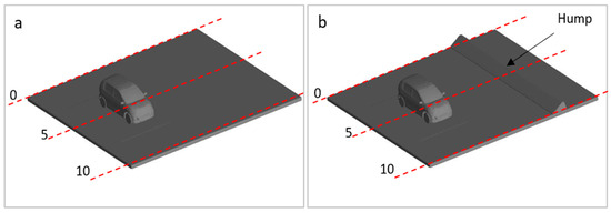
Figure 10.
Geometry output after running FAVOR solver (a) subcritical setup (b) supercritical setup.
Table 2.
Details of numerical runs under subcritical and supercritical flows.
3. Results and Discussion
3.1. Recognition of Sliding Instability Numerically
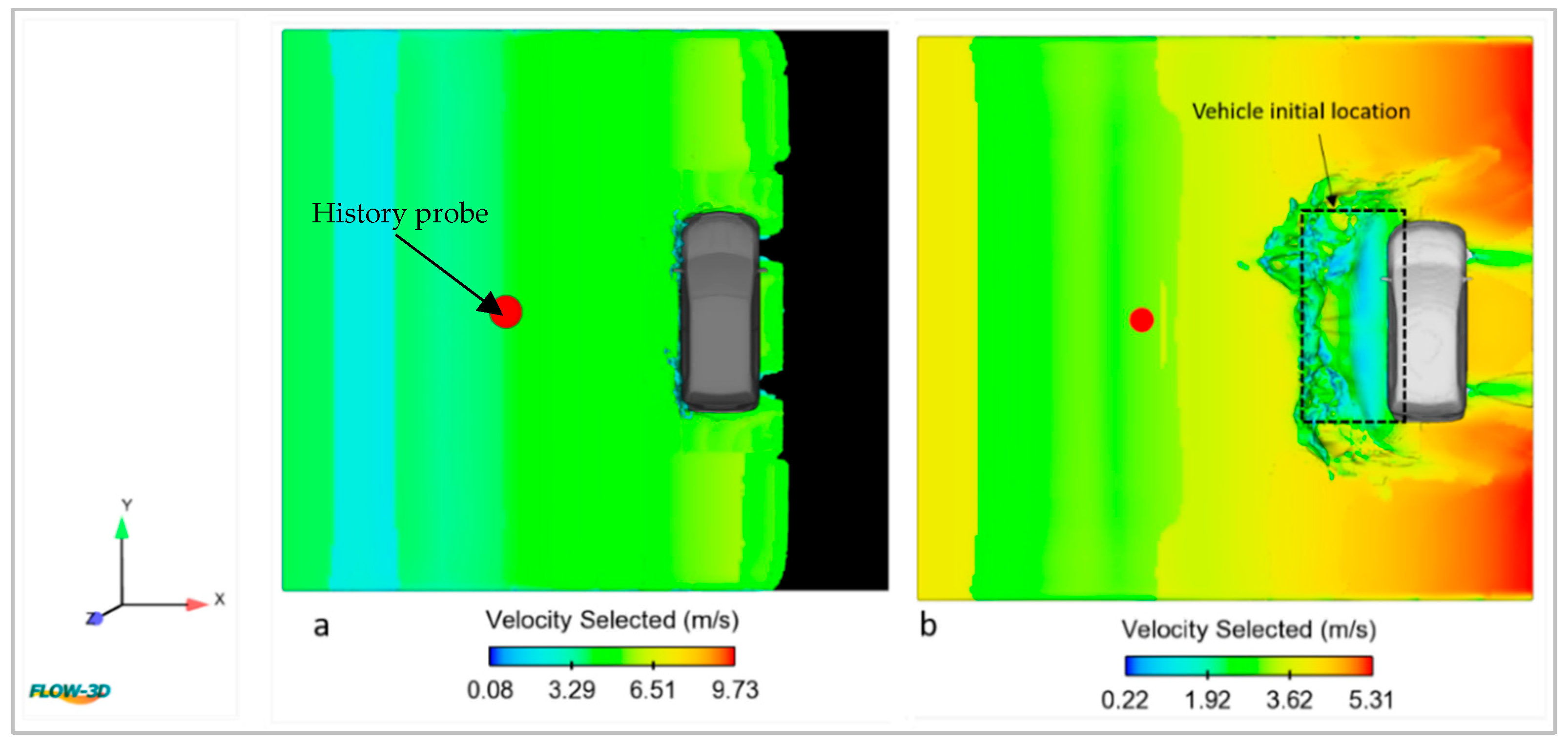
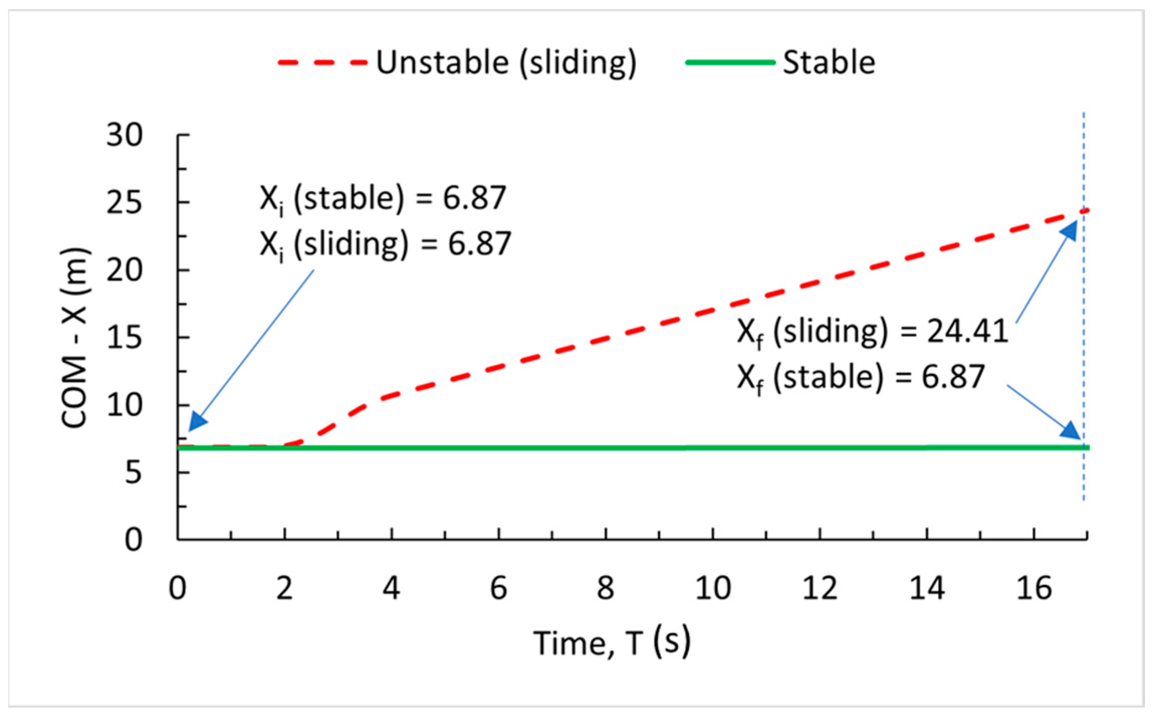
As mentioned earlier, the coupled motion simulation condition was used to run the numerical modelling. This setup allows the users to notice and detect the vehicle’s center of mass (COM) directly and identify whether the vehicle slid or not. In this study, stable and unstable conditions were recognized and recorded. Among the 14 numerical runs, it was found that the vehicle lost its stability under sliding mode in cases 1, 9, 10, and 11, while the floating instability occurred in cases 12, 13, and 14, as shown in Table 2. Figure 10 and Figure 11 show the stable and unstable conditions obtained from the numeral simulation, respectively. From Figure 12, it can be noticed that the vehicle was dragged from its initial location, resulting in sliding instability. On the other hand, the vehicle model remained at its initial location in the stable condition, as shown in Figure 11. Moreover, COM in the x-direction (flow direction) was recorded for both stable and unstable conditions. Figure 13 shows the changes in the vehicle X-COM with time. It was clear that, for stable conditions, there were no changes in the vehicle X-COM value with the time at which the initial and final x coordinates were xi = 6.87 m and xf = 6.88 m, respectively. On the other hand, the vehicle X-COM values changed significantly with time resulting in the sliding instability mode and the initial and final x coordinates were xi = 6.87 m and xf = 24.41 m, respectively.
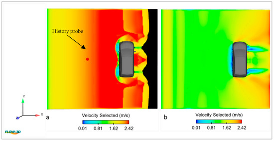
Figure 11.
Vehicle at stable condition case #8 (a) time = 4 s, (b) time= 16 s (end of computation).
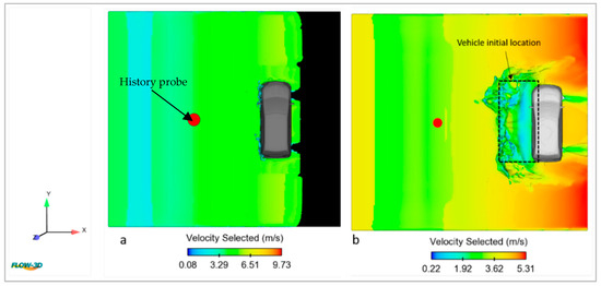
Figure 12.
Sliding instability occurrence in numerical simulation case #11 (a) time = 2 s (before sliding), (b) time = 3.5 s (after sliding).
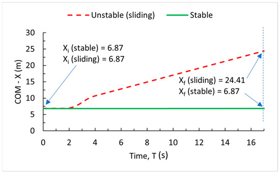
Figure 13.
Relationship between vehicle center of mass in x-direction and time.
3.2. Streamlines Distribution
The distribution of the streamlines around the vehicle body for the steady-state condition under subcritical flows can be seen in Figure 14. It was observed that the streamlines were redirected and became more complex near tires. resulting in reduced velocity magnitudes behind the tires, as shown in Figure 14. The flow velocity underneath the vehicle increased due to the ground clearance distance.
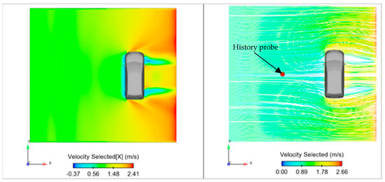
Figure 14.
Streamlines around the car for supercritical flows.
3.3. Hydrodynamic Forces
In FLOW-3D, the pressure magnitude on all vehicle faces including the bottom and sides were measured and recorded at every time step. Later, the forces acting on the vehicle were computed by integrating the pressures on the surface based on the recorded pressure and affected area.
3.3.1. Horizontal Force, FH
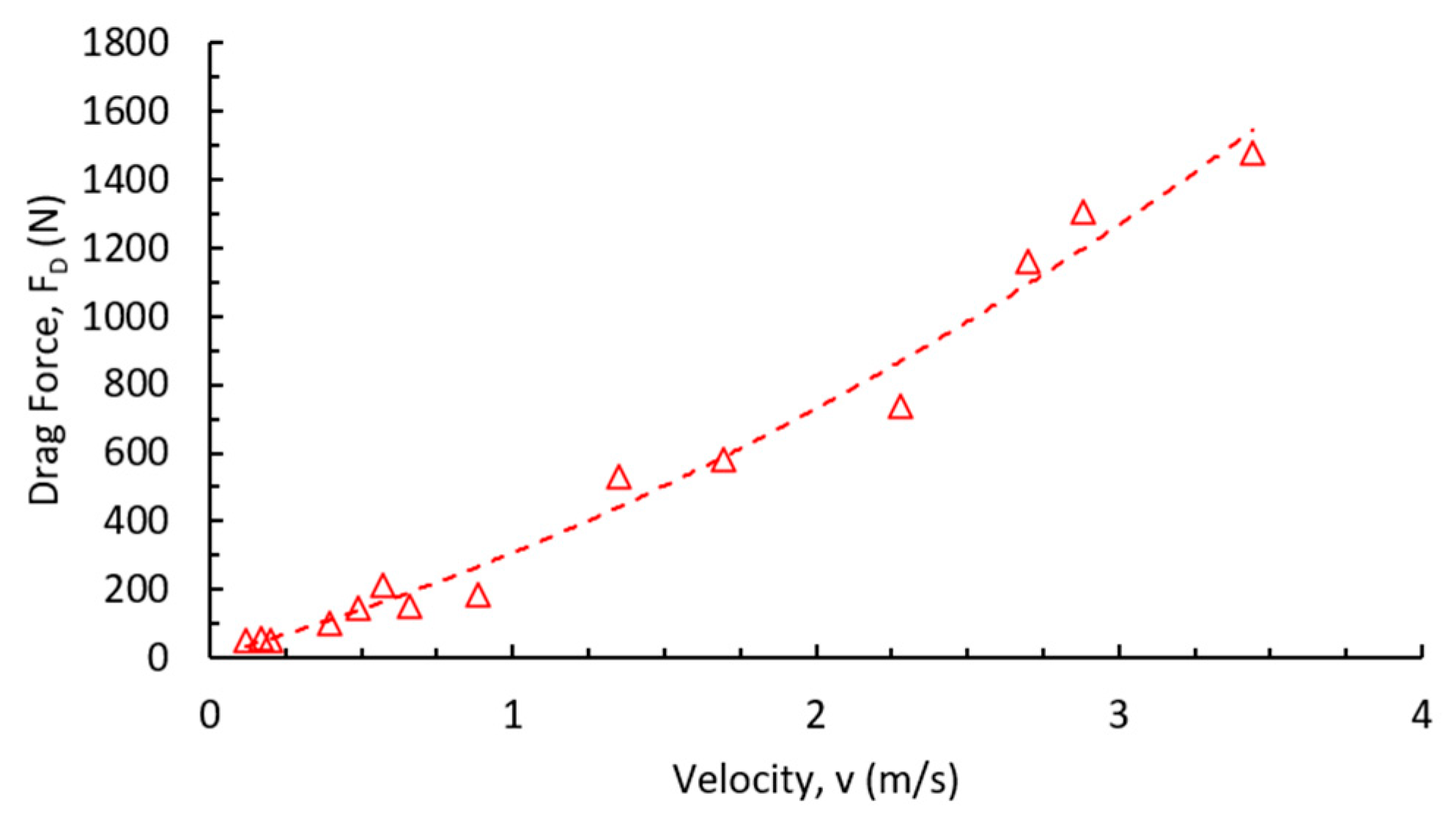
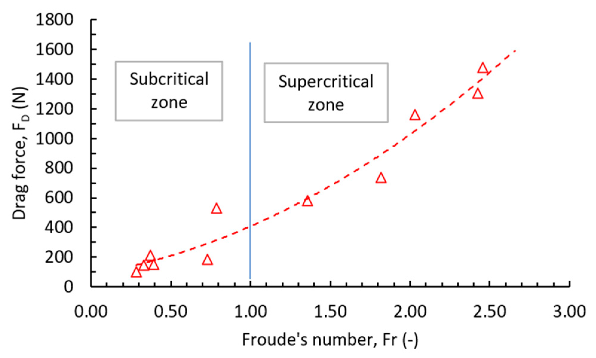
The horizontal force is mainly accounted as the cause of the sliding instability mode and it is mainly governed by the flow velocity, affected area, and drag coefficient. Figure 15 and Figure 16 show the relationships between the drag force and flow velocity and drag force and Froude number, respectively. From both figures, it can clearly be seen that the drag force increases with the increment of both parameters as expected. Further, it was observed that the increment of drag force was gradual at low flow velocity and Froude number, while at higher values the drag force increased significantly. As mentioned earlier, the sliding instability mode is governed by the values of drag and friction forces; thus, the vehicle will be in more danger of sliding under supercritical flows when compared with conditions under subcritical flows. From the results, it can be concluded that the sliding instability mode mainly occurs under supercritical flows when Froude numbers are more than 1.

Figure 15.
Relationship between drag force and flow velocity.

Figure 16.
Relationship between drag force and Froude number.
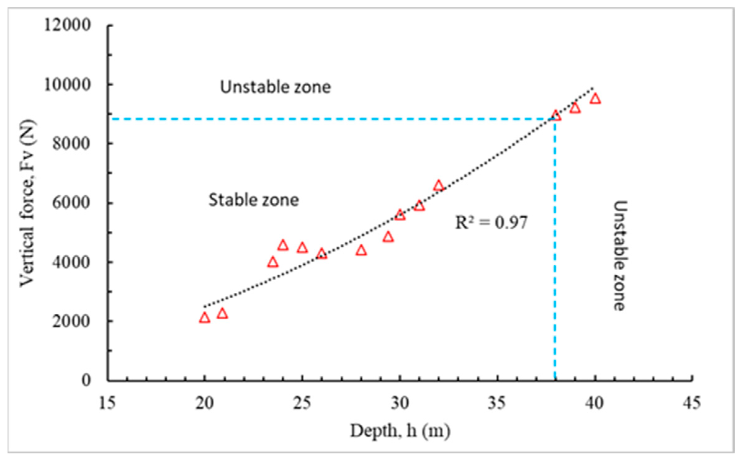
3.3.2. Vertical Force, FV
Vertical force corresponds to the pushing-up pressure exerted by the flow against the vehicle’s weight. It is considered as the main force causing the floating instability modes and it is mainly governed by the water depth at the vehicle vicinity. Herein, the relationship between water depth and buoyancy force was considered rather than other flow parameters. Numerical results revealed that the vertical force increased gradually with the increment of water depth, as shown in Figure 17. The vehicle was seen to float once the water depth at the vehicle vicinity was more than 0.38 m and the buoyancy force was 9.16 KN. From Figure 17, a power equation (Equation (9)) describing the relationship between vertical force (Fv) and water depth (h) can be proposed as follows:
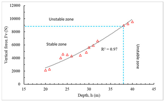
Figure 17.
Relationship between vertical force and flow depth.
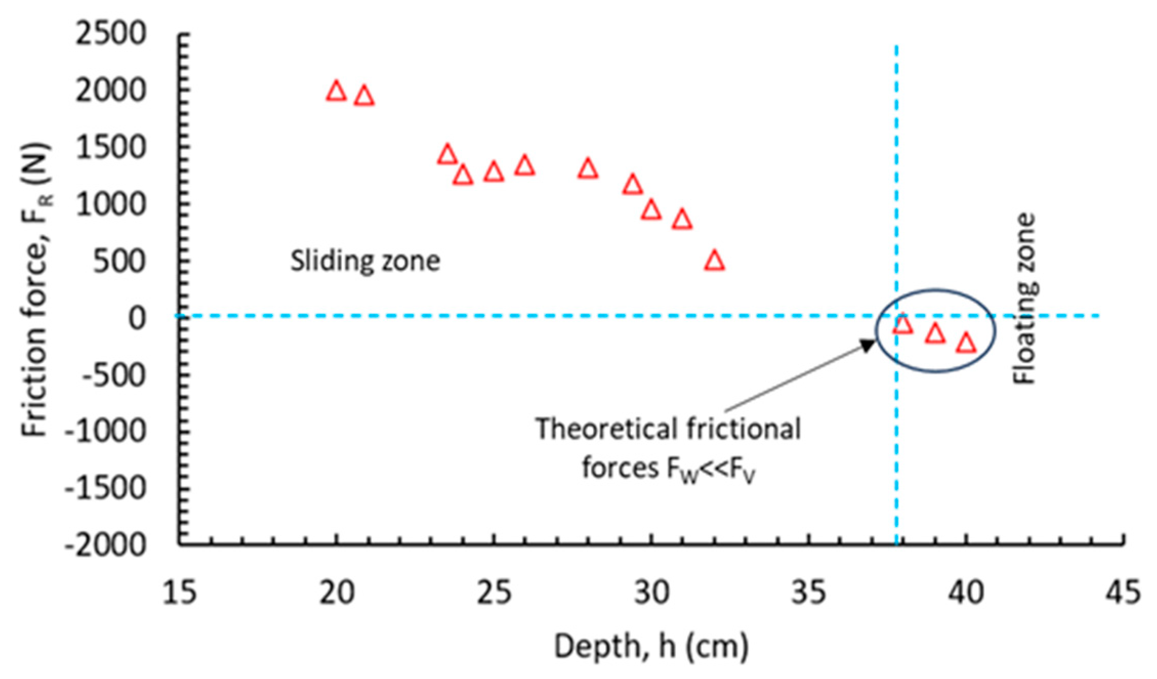
3.3.3. Frictional Force, FR
The frictional force exists due to the contact between the ground surface and the tires. Among the other numerical simulation setups, the static friction coefficient of the road was set to be 0.30 following the experimental results obtained by Bonham and Hattersley (1967) [8], Gordon and Stone (1973) [10]. Later, the frictional force was calculated using Equation (11) based on the measured vertical force and vehicle weight. The results showed that the friction force decreased with the increment of flow depth, as shown in Figure 18. The negative values in Figure 18 represent the theoretical frictional forces which were calculated using Equation (10). The negative values indicated that the vehicle was under floating instability mode and there was no more contact between the ground surface and the vehicle tires, i.e., the upward pushing force was more than the vehicle weight (FV >> FW):
where µ is the friction coefficient, FW is the vehicle weight under dry conditions, and FV is the upward pushing force.
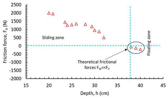
Figure 18.
Relationship between frictional force and Froude number.
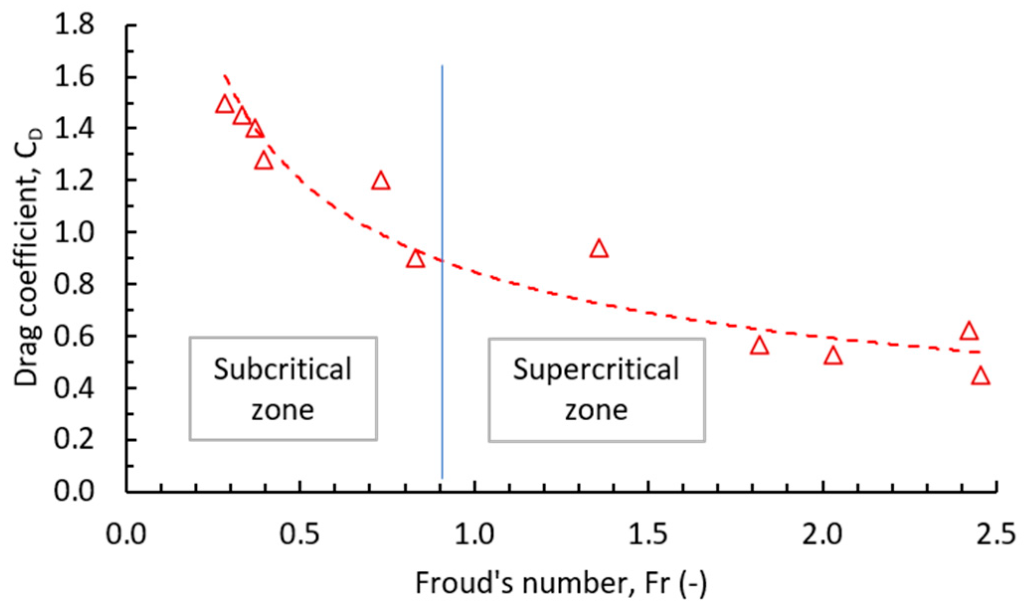
3.3.4. Drag Coefficient, CD
For a static vehicle at a 90° orientation, the main drag coefficient is the one calculated from the drag force that has an effect on the vehicle’s longitudinal side (Equation (11)). The numerical results revealed that the drag coefficient CD decreased with the increment of the Froude number, as shown in Figure 19. At low Froude numbers (subcritical flows), the drag coefficients were higher than 1. However, at high Froude numbers (supercritical flows), the drag coefficients were found to be less than 1. It can then be concluded that the drag coefficient is not constant as proposed in earlier experimental studies, but changes with Froude numbers and flow conditions:
where FH is the drag force, ρ is the water density, AD is the affected area projected normally to the incoming flow, and v is the flow velocity.
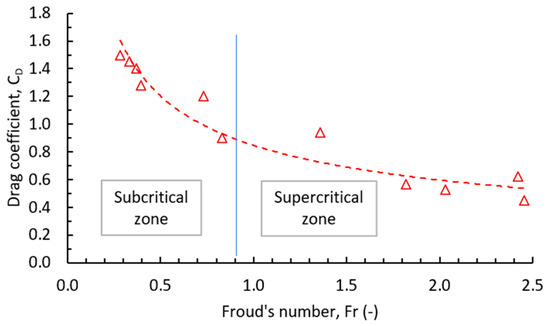
Figure 19.
Relationship between drag coefficient and Froude number.
4. Validation of Results
For validation purposes, the obtained numerical results discussed in the present study were compared with three previously published works. Firstly, the stable and unstable scenarios which were predicted numerically were compared with the Australian Rainfall and Runoff (AR&R 2011) [32] guidelines for small and medium passenger vehicles to evaluate the reliability of the proposed numerical framework (see Section 4.1). Secondly, the floating depth and the threshold function obtained in this study were compared with the theoretical equations proposed by Martínez-Gomariz et al. (2017) [13] (see Section 4.2). Finally, the hydrodynamic forces on the flooded vehicle obtained in the present study were compared with the results reported by Al-Qadami et al. (2022) [33].
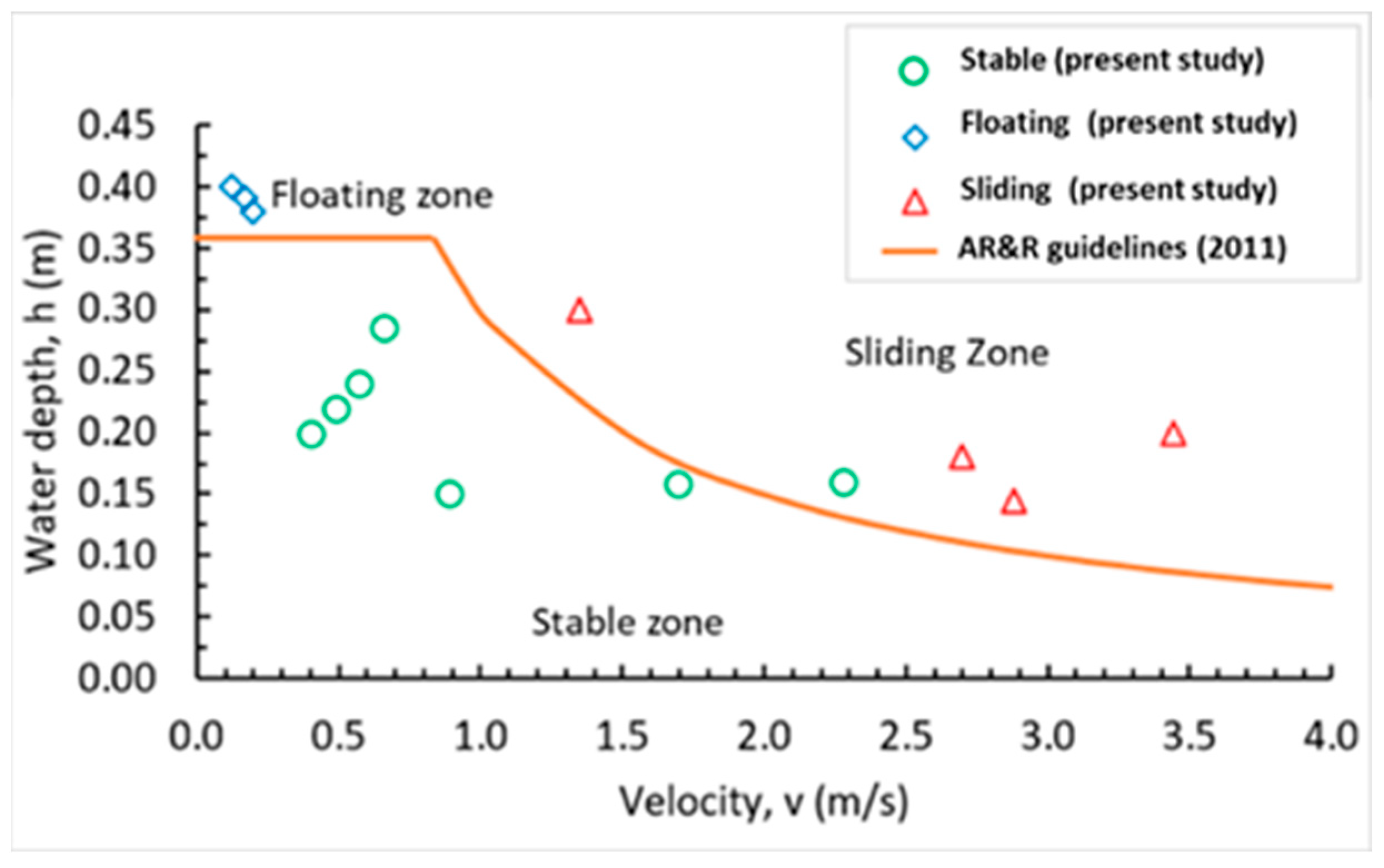
4.1. Australian Rainfall and Runoff (AR&R 2011) [32]
A comparison between the obtained numerical simulation results and previously published guidelines by Australian Rainfall and Runoff (AR&R 2011) was conducted, as shown in Figure 20. It can be seen that the obtained numerical results under six degrees of freedom and coupled motion conditions strongly agree with the published guidelines. The floating and sliding numerical cases obtained in this study were located above the stability threshold at which the unstable zone was defined, while the stable cases were located underneath the stability chart. However, there is one case that was observed as stable according to the numerical simulation, but it was located in the unstable zone, as shown in Figure 20.

Figure 20.
Comparison between the obtained results and AR&R guidelines [32] for small and medium vehicles.
4.2. Martínez-Gomariz et al. (2017) [13]
The threshold function (Equation (12)) and floating depth equation (Equation (13)) that was proposed by Martínez-Gomariz et al. (2017) [13]) was used to validate the minimum threshold velocity and floating depth, respectively. It was noticed that the minimum threshold velocity obtained from (Equation (12)) was 0.47 m2/s, while it was 0.36 m2/s in this numerical study with a percentage difference of 25%. On the other hand, it was found that the floating depth calculated from (Equation (13)) was 0.368 m, while the floating depth that was obtained numerically in this study was 0.380 m. A strong agreement between both results was noticed with a difference percentage of 3.20%:
where hb is the buoyancy depth, Mc is the vehicle weight, ρ is the fluid density, lc and bc are the length and width of the vehicle, respectively, GC is the vehicle ground clearance, PA is the vehicle plane area, and is the friction coefficient.
4.3. Al-Qadami et al. (2022) [33]
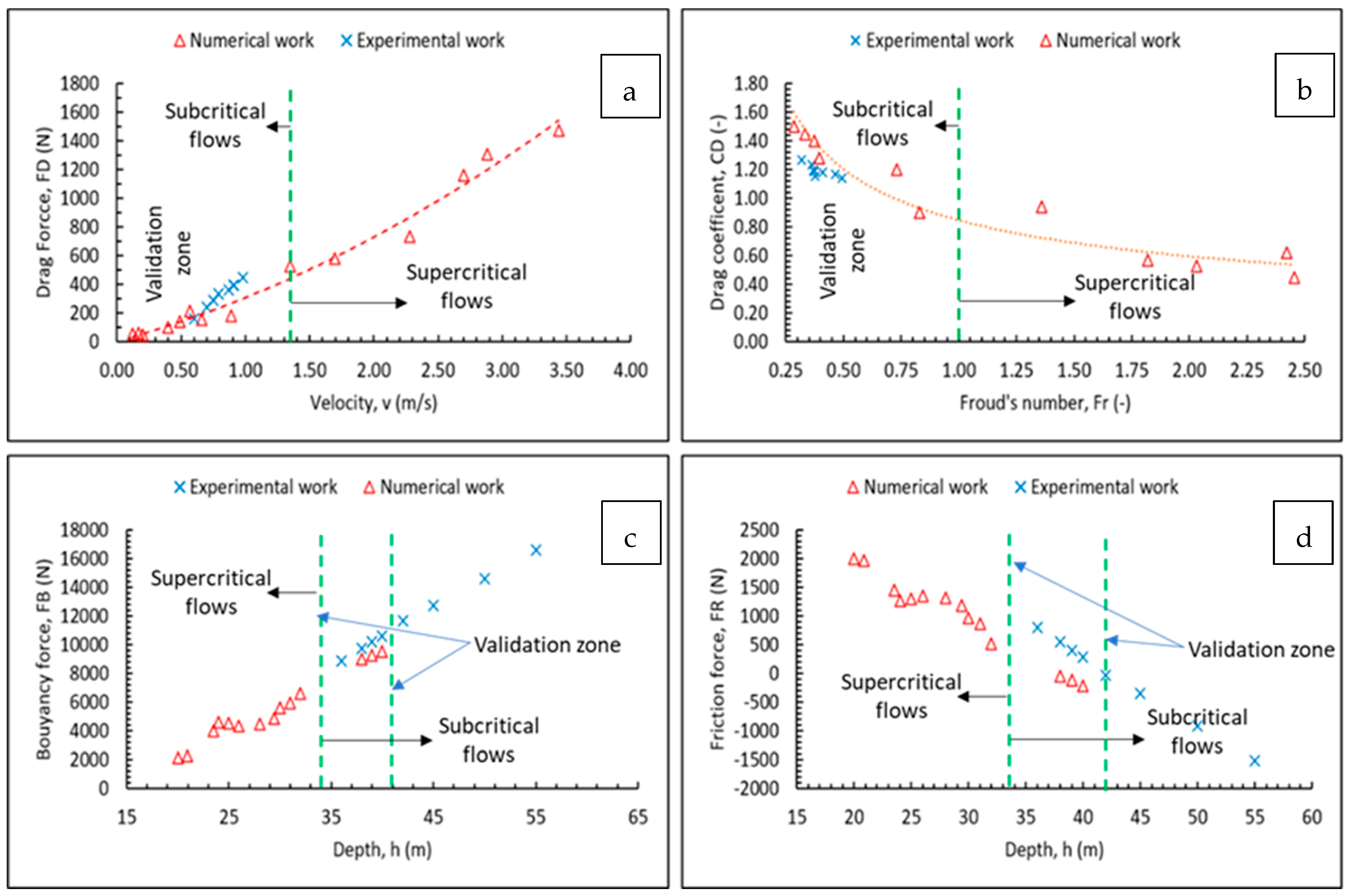
The obtained numerical results were further compared with the experimental results that were introduced by Al-Qadami et al. (2022) [33]. The experimental study was performed for the same vehicle model (Peruodu Viva) but only under subcritical flow conditions. Figure 21 shows the comparison between the current numerical results and the published experimental results in terms of hydrodynamic forces. It can be seen that both results properly aligned with each other, especially the relationships between (i) drag coefficient and Froude number, (ii) buoyancy force and water depth, and (iii) frictional force and water depth, as shown in Figure 21b–d, respectively. However, the numerical and experimental results trend of drag force and flow velocity (Figure 21a) was not accurately aligned; this could be due to the limitations of the experimental study which only covered the subcritical flow regime. Overall, this comparison process indicates that the numerical framework proposed in this study can be considered a reliable method to be used in future studies dealing with flooded vehicle instability.
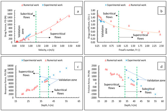
Figure 21.
Comparison between obtained numerical findings and experimental results reported by Al-Qadami et al. (2022) [33].
5. Conclusions
In this paper, numerical modelling was conducted to assess the stability of a full-scale passenger vehicle during floodwaters. For the purpose of modelling, a medium passenger vehicle called Peruodu Viva was selected and exposed to different combinations of flow velocities and water depths with a Froude number range between 0.09 and 2.46. The numerical simulation in the present study was performed under six degrees of freedom and fully coupled motion set-ups. Based on the obtained results, the following conclusions were drawn:
- For the tested vehicle model, it was noticed that the floating instability mode occurred once the upward pushing forces exceeded the vehicle weight as expected. On the other hand, the sliding instability mode occurred once the horizontal drag force exceeded the frictional resistance between the tires and the ground surface.
- The sliding instability mode was observed in four cases with the depth × velocity threshold function values of 0.41, 0.40, 0.49, and 0.69 m2/s, while the floating instability mode was observed in three cases when water depth reached more than 0.38 m.
- The threshold value of the depth × velocity function was found to be 0.36 m2/s, at which the vehicle was considered stable if m2/s, while the vehicle lost its stability if m2/s.
- The floating instability mode was common when the flow was subcritical, while the sliding stability mode was common when the flow was supercritical.
- Both instability modes could occur at the same time, i.e., the vehicle floated first and then was washed away within the flow direction.
- The drag force was mainly influenced by the flow velocity while the buoyancy force was mainly affected by the water depth at the vehicle vicinity.
- The drag coefficient was observed to be more than 1 when the flow was subcritical, but the value was reduced to less than 1 when the flow was supercritical.
- By employing six degrees of freedom and fully coupled techniques, the vehicle center of mass could be detected at each time step. This helped to accurately know whether the vehicle was stable or not.
- The validation process showed that the obtained numerical results were logical, and the proposed numerical framework was reliable in predicting the stability limits of any other vehicles.
The authors believe that the proposed numerical framework presented in this study can help to redirect the research approaches regarding flooded vehicle stability studies. However, it is recommended to extend this work by conducting more numerical modelling by adopting different road surface friction coefficients, different vehicle models, and orientations against the incoming flow to confirm the accuracy of the presented numerical framework.
Author Contributions
Conceptualization, E.H.H.A.-Q., Z.M. and E.M.-G.; methodology, E.H.H.A.-Q., Z.M. and E.M.-G.; software, Z.M.; validation, E.H.H.A.-Q., Z.M. and M.A.M.R.; formal analysis, E.H.H.A.-Q.; investigation, E.H.H.A.-Q. and M.A.M.R.; resources, E.H.H.A.-Q., Z.M. and W.S.D.; data curation, E.H.H.A.-Q.; writing—original draft preparation, E.H.H.A.-Q.; writing—review and editing, E.H.H.A.-Q., M.A.M.R., W.S.D., Z.M. and E.M.-G.; visualization, M.A.M.R., W.S.D. and Z.M.; supervision, M.A.M.R. and Z.M.; project administration, Z.M.; funding acquisition, W.S.D. All authors have read and agreed to the published version of the manuscript.
Funding
This research was supported by the Institute for Research and Community Service, Universitas Muhammadiyah Sumatera Utara “Lembaga Penelitian dan Pengabdian Masyarakat, Universitas Muhammadiyah Sumatera Utara”.
Institutional Review Board Statement
Not applicable.
Informed Consent Statement
Not applicable.
Data Availability Statement
The data presented in this study are available on request from the corresponding author.
Acknowledgments
The authors acknowledge the Universiti Teknologi PETRONAS (UTP), Malaysia, and Universiti Tun Hussein Onn Malaysia (UTHM), for providing the enabling environment to be utilized for this research.
Conflicts of Interest
The authors declare no conflict of interest.
Nomenclature
| VF | fluid volume function |
| ρ | fluid density (kg/m3) |
| t | time (s) |
| u | velocity components in the coordinate directions of x |
| v | velocity components in the coordinate directions of y |
| w | velocity components in the coordinate directions of z |
| RSOR | density source term |
| Ax | fractional area open to flow in the x direction |
| Ay | fractional area open to flow in the y direction |
| Az | fractional area open to flow in the z direction |
| Gx | body acceleration in x coordinate |
| Gy | body acceleration in y coordinate |
| Gz | body acceleration in z coordinate |
| fx | viscous accelerations in the x direction |
| fy | viscous accelerations in the y direction |
| fz | viscous accelerations in the z direction |
| P | pressure (Pa) |
| GT | buoyancy production term |
| ϵT | energy dissipation rate |
| PT | turbulence kinetic energy |
| DiffKT | diffusion term |
| CDIS1 | dimensionless user-adjustable parameters |
| CDIS2 | dimensionless user-adjustable parameters |
| CDIS3 | dimensionless user-adjustable parameters |
| hb | buoyancy depth |
| Mc | vehicle weight |
| Lc | vehicle length |
| bc | vehicle width |
| GC | ground clearance, |
| PA | vehicle plane area |
| μ | friction coefficient |
| FR | frictional force |
| FW | vehicle weight |
| FV | upward pushing force (vertical force) |
| CD | drag coefficient |
| FH | drag force |
| AD | area projected normally to the incoming flow |
| H | water depth |
References
- Enríquez-de-Salamanca, Á. Victims crossing overflowing watercourses with vehicles in Spain. J. Flood Risk Manag. 2020, 13, e12645. [Google Scholar] [CrossRef]
- Ashley, S.T.; Ashley, W.S. Flood fatalities in the United States. J. Appl. Meteorol. Climatol. 2008, 47, 805–818. [Google Scholar] [CrossRef]
- Drobot, S.D.; Benight, C.; Gruntfest, E.C. Risk factors for driving into flooded roads. Environ. Hazards 2007, 7, 227–234. [Google Scholar] [CrossRef]
- Diakakis, M.; Deligiannakis, G. Vehicle-related flood fatalities in Greece. Environ. Hazards 2013, 12, 278–290. [Google Scholar] [CrossRef]
- Petrucci, O.; Salvati, P.; Aceto, L.; Bianchi, C.; Pasqua, A.A.; Rossi, M.; Guzzetti, F. The vulnerability of people to damaging hydrogeological events in the Calabria Region (Southern Italy). Int. J. Environ. Res. Public Health 2018, 15, 48. [Google Scholar] [CrossRef] [PubMed]
- Petrucci, O.; Papagiannaki, K.; Aceto, L.; Boissier, L.; Kotroni, V.; Grimalt, M.; Llasat, M.C.; Llasat-Botija, M.; Rosselló, J.; Pasqua, A.A. MEFF: The database of Mediterranean flood fatalities (1980 to 2015). J. Flood Risk Manag. 2019, 12, e12461. [Google Scholar] [CrossRef]
- Ahmed, M.A.; Haynes, K.; Taylor, M. Vehicle-related flood fatalities in Australia, 2001–2017. J. Flood Risk Manag. 2020, 13, e12616. [Google Scholar] [CrossRef]
- Bonham, A.J.; Hattersley, R.T. Low level causeways [Technical Report 100]; The University of New South Wales, Water Research Laboratory: Sydney, Australia, 1967. [Google Scholar]
- Smith, G.P.; Modra, B.D.; Felder, S. Full-scale testing of stability curves for vehicles in flood waters. J. Flood Risk Manag. 2019, 12, e12527. [Google Scholar] [CrossRef]
- Gordon, A.D.; Stone, P.B. Car Stability on Road Floodways. National Capital Development Commission; Report; National Library of Australia: Parkes, Australia, 1973. [Google Scholar]
- Shand, T.D.; Smith, G.P.; Cox, R.J.; Blacka, M. Development of Appropriate Criteria for the Safety and Stability of Persons and Vehicles in Floods. In Proceedings of the 34th World Congress of the International Association for Hydro-Environment Research and Engineering: 33rd Hydrology and Water Resources Symposium and 10th Conference on Hydraulics in Water Engineering, Brisbane, Australia, 26 June–1 July 2011. [Google Scholar]
- Kramer, M.; Terheiden, K.; Wieprecht, S. Safety criteria for the trafficability of inundated roads in urban floodings. Int. J. Disaster Risk Reduct. 2016, 17, 77–84. [Google Scholar] [CrossRef]
- Martínez-Gomariz, E.; Gómez, M.; Russo, B.; Djordjević, S. A new experiments-based methodology to define the stability threshold for any vehicle exposed to flooding. Urban Water J. 2017, 14, 930–939. [Google Scholar] [CrossRef]
- Shu, C.; Xia, J.; Falconer, R.A.; Lin, B. Incipient velocity for partially submerged vehicles in floodwaters. J. Hydraul. Res. 2011, 49, 709–717. [Google Scholar] [CrossRef]
- Teo, F.Y.; Xia, J.; Falconer, R.A.; Lin, B. Experimental studies on the interaction between vehicles and floodplain flows. Int. J. River Basin Manag. 2012, 10, 149–160. [Google Scholar] [CrossRef]
- Al-Qadami, E.H.H.; Razi, M.A.M.; Damanik, W.S.; Mustaffa, Z.; Martinez-Gomariz, E.; Teo, F.Y.; Saeed, A.A.H. 3-Dimensional Numerical Study on the Critical Orientation of the Flooded Passenger Vehicles. Eng. Lett. 2023, 31, 961–968. [Google Scholar]
- Xia, J.; Falconer, R.; Lin, B.; Tan, G. Numerical assessment of flood hazard risk to people and vehicles in flash floods. Environ. Model. Softw. 2011, 26, 987–998. [Google Scholar] [CrossRef]
- Arrighi, C.; Alcèrreca-huerta, J.C.; Oumeraci, H.; Castelli, F. Drag and lift contribution to the incipient motion of partly submerged flooded vehicles. J. Fluids Struct. 2015, 57, 170–184. [Google Scholar] [CrossRef]
- Albano, R.; Sole, A.; Mirauda, D.; Adamowski, J. Modelling large floating bodies in urban area flash-floods via a Smoothed Particle Hydrodynamics model. J. Hydrol. 2016, 541, 344–358. [Google Scholar] [CrossRef]
- Amicarelli, A.; Albano, R.; Mirauda, D.; Agate, G.; Sole, A.; Guandalini, R. A Smoothed Particle Hydrodynamics model for 3D solid body transport in free surface flows. Comput. Fluids 2015, 116, 205–228. [Google Scholar] [CrossRef]
- Gómez, M.; Martínez, E.; Russo, B. Experimental and Numerical Study of Stability of Vehicles Exposed to Flooding. In Advances in Hydroinformatics; Springer: Berlin/Heidelberg, Germany, 2018; pp. 595–605. [Google Scholar]
- Martínez-Gomariz, E.; Gómez, M.; Russo, B. Estabilidad de vehículos frente a inundaciones: Estudio numérico-experimental. Ribagua 2019, 6, 123–137. [Google Scholar] [CrossRef]
- Al-Qadami, E.H.H.; Mustaffa, Z.; Al-Atroush, M.E.; Martinez-Gomariz, E.; Teo, F.Y.; El-Husseini, Y. A numerical approach to understand the responses of passenger vehicles moving through floodwaters. J. Flood Risk Manag. 2022, 15, e12828. [Google Scholar] [CrossRef]
- Al-Qadami, E.H.H.; Mustaffa, Z.; Martínez-Gomariz, E.; Yusof, K.W.; Abdurrasheed, A.S.; Shah, S.M.H. Numerical Simulation to Assess Floating Instability of Small Passenger Vehicle Under Sub-critical Flow. In Proceedings of the International Conference on Civil, Offshore and Environmental Engineering, Dubai, United Arab Emirates, 20–21 December 2021; Springer: Berlin/Heidelberg, Germany, 2021; pp. 258–265. [Google Scholar]
- Mustaffa, Z.; Al-Qadami, E.H.H.; Shah, S.M.H.; Yusof, K.W. Impact and Mitigation Strategies for Flash Floods Occurrence towards Vehicle Instabilities. In Flood Impact Mitigation and Resilience Enhancement; IntechOpen: London, UK, 2020. [Google Scholar]
- Abdurrasheed, S.; Wan Yusof, K.; Hamid Hussein Alqadami, E.; Takaijudin, H.; Muhammad, M.M.; Sholagberu, A.T.; Zainalfikry, M.K.; Osman, M.; Shihab Patel, M. Modelling of flow parameters through subsurface drainage modules for application in BIOECODS. Water 2019, 11, 1823. [Google Scholar] [CrossRef]
- Maldar, N.R.; Ng, C.Y.; Ean, L.W.; Oguz, E.; Fitriadhy, A.; Kang, H.S. A Comparative Study on the Performance of a Horizontal Axis Ocean Current Turbine Considering Deflector and Operating Depths. Sustainability 2020, 12, 3333. [Google Scholar] [CrossRef]
- Wahyudi, B.; Adiwidodo, S. The influence of moving deflector angle to positive torque on the hydrokinetic cross flow savonius vertical axis turbine. Int. Energy J. 2017, 17, 11–21. [Google Scholar]
- Barkhudarov, M.R. Lagrangian VOF Advection method for FLOW-3D. Flow Sci. Inc. 2004, 1. Available online: https://citeseerx.ist.psu.edu/document?repid=rep1&type=pdf&doi=693db5d4396e86fdf9850e282563950211a1d749 (accessed on 20 June 2023).
- Maguire, A.E. Hydrodynamics, Control and Numerical Modelling of Absorbing Wavemakers. Ph.D. Thesis, University of Edinburgh, Edinburgh, UK, 2011. [Google Scholar]
- Abu-Zidan, Y.; Mendis, P.; Gunawardena, T. Optimising the computational domain size in CFD simulations of tall buildings. Heliyon 2021, 7, e06723. [Google Scholar] [CrossRef] [PubMed]
- Shand, T.D.; Cox, R.J.; Blacka, M.J.; Smith, G.P. Australian Rainfall and Runoff Project 10: Appropriate Safety Criteria for Vehicles–Literature Review. Commonw. Aust. Geoscience Aust. 2011, 2, 1–29. [Google Scholar]
- Al-Qadami, E.H.H.; Mustaffa, Z.; Shah, S.M.H.; Matínez-Gomariz, E.; Yusof, K.W. Full-scale experimental investigations on the response of a flooded passenger vehicle under subcritical conditions. Nat. Hazards 2022, 110, 325–348. [Google Scholar] [CrossRef]
Disclaimer/Publisher’s Note: The statements, opinions, and data contained in all publications are solely those of the individual author(s) and contributor(s) and not of MDPI and/or the editor(s). MDPI and/or the editor(s) disclaim responsibility for any injury to people or property resulting from any ideas, methods, instructions, or products referred to in the content. |


Disclaimer/Publisher’s Note: The statements, opinions and data contained in all publications are solely those of the individual author(s) and contributor(s) and not of MDPI and/or the editor(s). MDPI and/or the editor(s) disclaim responsibility for any injury to people or property resulting from any ideas, methods, instructions or products referred to in the content. |
© 2023 by the authors. Licensee MDPI, Basel, Switzerland. This article is an open access article distributed under the terms and conditions of the Creative Commons Attribution (CC BY) license (https://creativecommons.org/licenses/by/4.0/).